Phytoplankton Phenology in the Coastal Zone of Cyprus, Based on Remote Sensing and In Situ Observations

Abstract

Alterations in phytoplankton biomass, community structure and timing of their growth (phenology), are directly implicated in the carbon cycle and energy transfer to higher trophic levels of the marine food web. Due to the lack of long-term in situ datasets, there is very little information on phytoplankton seasonal succession in Cyprus (eastern Mediterranean Sea). On the other hand, satellite-derived measurements of ocean colour can only provide long-term time series of chlorophyll (an index of phytoplankton biomass) up to the first optical depth (surface waters). The coupling of both means of observations is essential for understanding phytoplankton dynamics and their response to environmental change. Here, we use 23 years of remotely sensed, regionally tuned ocean-colour observations, along with a unique time series of in situ phytoplankton pigment composition data, collected in coastal waters of Cyprus during 2016. The satellite observations show an initiation of phytoplankton growth period in November, a peak in February and termination in April, with an overall mean duration of ~4 months. An in-depth exploration of in situ total Chl-a concentration and phytoplankton pigments revealed that pico- and nano-plankton cells dominated the phytoplankton community. The growth peak in February was dominated by nanophytoplankton and potentially larger diatoms (pigments of 19’ hexanoyloxyfucoxanthin and fucoxanthin, respectively), in the 0–20 m layer. The highest total Chl-a concentration was recorded at a station off Akrotiri peninsula in the south, where strong coastal upwelling has been reported. Another station in the southern part, located next to a fish farm, showed a higher contribution of picophytoplankton during the most oligotrophic period (summer). Our results highlight the importance of using available in situ data coupled to ocean-colour remote sensing, for monitoring marine ecosystems in areas with limited in situ data availability.

1. Introduction

The eastern Mediterranean Sea is characterised as an ultraoligotrophic region, comparable to the most oligotrophic parts of the global ocean, and is even considered as a marine desert [1,2]. This ultraoligotrophic nature is reflected in the very low primary production, chlorophyll-a (Chl-a, a proxy of phytoplankton biomass [3]) and nutrient concentrations, predominance of small-sized phytoplankton and its extremely clear waters [4,5,6,7,8,9,10,11]. Cyprus, the third largest island in the Mediterranean, located in the Levantine Basin, has a highly exposed coastline and very narrow shelf area, implying that coastal conditions may not significantly differ and thus be representative of the physicochemical regime of the open waters [12]. The ultraoligotrophic character of the eastern Mediterranean is also documented in Cyprus’ coastal waters, through coastal stations’ monitoring by the Department of Fisheries and Marine Research (DFMR) as part of the implementation of the European Marine Strategy Framework Directive (MSFD, 2008/56/EC) [13]. Average mineral nutrient concentrations in the surface layers are at the low end of the global coastal concentration ranges [12]. Further, Chl-a values showed some of the lowest concentrations ever recorded in coastal waters (0.01–0.09 μg/L) [14]. Another characteristic of Cyprus’ coastal waters is the extremely limited runoff. In addition, due to the increased drought incidents, 108 dams have been constructed in almost all the streams of the country [15,16], leading to an overexploitation (by 40%) of groundwater resources [17], further limiting the natural supply of coastal waters with nutrients.

Phytoplankton are responsible for approximately half of the total global primary production [18,19], directly implicated in the carbon cycle and energy transfer to higher trophic levels, supporting marine food webs by providing an essential food source for many commercially important fish species’ larvae and juveniles [20]. Phytoplankton phenology metrics, such as growth initiation, time of maximum amplitude, duration and termination, are categorised as ecological indicators [21]. Phenology metrics are a key factor in determining the structure of food webs and ecosystem function [22,23]. Monitoring these indicators offers a way to observe the response of marine ecosystems to environmental change [21,22,24,25]. Marine phytoplankton play a fundamental role in climate regulation through carbon cycling. Alterations in phytoplankton abundance and composition driven by climate change may alter marine biogeochemical cycles, with far reaching consequences for the marine environment [26]. Further, oceanic warming may cause mismatches between marine organisms’ reproductive cycles and their planktonic diet [27]. According to the match/mismatch hypothesis, fish stock recruitment depends on the synchronous production of food [28], and any interannual variations in phytoplankton phenology can have widespread ecosystem implications. Therefore, changes in the phytoplankton phenology can have detrimental cascade effects on the survival of commercially important species [27,29,30].

Despite the significance of phytoplankton in the functioning of marine ecosystems, the seasonal succession of phytoplankton in Cyprus’ coastal waters has yet to be determined, primarily due to the lack of in situ measurements. The only study to determine Chl-a and carotenoids based on a High-Performance Liquid Chromatography (HPLC) method took place in June and July 1993, where the dominant phytoplankton classes were determined to be chlorophytes, cyanobacteria and prochlorophytes, based on chlorophyll-b and zeaxanthin concentrations [14].

Alternatively, ocean-colour remote sensing provides long-term monitoring of Chl-a concentrations. Therefore, measuring Chl-a concentration using remote sensing can assess phytoplankton ecological indicators and characterise the status of marine ecosystems [21,24]. Since knowledge on long-term and large-scale data on phytoplankton phenology based on in situ data in Cyprus is not available, ocean-colour remote sensing offers the only means to obtain such information in this area. However, satellite observations are limited in determining only total Chl-a at the surface and do not offer information on the contribution of individual pigments to TChl-a. Knowledge of the pigment composition is important for assessing the composition of phytoplanktonic communities, since most of the pigments have chemotaxonomic associations (i.e., they are biomarkers for specific phytoplankton groups), and may reflect the contribution of phytoplankton size classes (pico-, nano- and micro-phytoplankton) [11,31]. On the other hand, in situ measurements are limited in space and time. The synergy of both in situ and satellite observations may lead to a deeper understanding of phytoplankton dynamics in data-poor regions, such as the coastal waters of Cyprus.

Here, 23 years of remotely sensed ocean-colour observations are combined with a unique in situ time series of monthly biophysical datasets collected in the coastal waters of Cyprus in 2016, to investigate phytoplankton phenology, the associated pigment composition and their seasonal succession. Further, we investigate if coastal waters of Cyprus are indeed representative of the oligotrophic offshore waters of the eastern Mediterranean Sea.

2. Materials and Methods

2.1. Satellite Remote Sensing Data

The multisensor Chl-a (mg/m³) daily product at 1 km resolution was obtained from the EU Copernicus Marine Environment Monitoring Service (CMEMS) at https://marine.copernicus.eu/ (accessed on 1 July 2021) that is a merge of MODIS-Aqua, NOAA-20-VIIRS, NPP-VIIRS, Sentinel3A-OLCI data, covering the time period from September 1997 to December 2020. The bio-optical algorithm used to estimate Chl-a concentration is a combination of MedOC4 for Case 1 [32] and AD4 for Case 2 waters [33], regionally tuned for the Mediterranean Sea. We note that remotely sensed ocean-colour algorithms have known limitations in shallow oligotrophic waters, generally resulting in an overestimation in chlorophyll concentrations [34,35,36]. We acknowledge that regardless of the usage of a regionally tuned algorithm (MEDOC4), there are still some slight discrepancies in comparison to our in situ datasets, especially during the most oligotrophic period (summer). Further validation of the currently available algorithms with additional ground-truth datasets could ultimately lead to an improved product.

The computation of the phenology metrics, as implemented in this study, follows the approach of Racault et al. [37]. First, we extracted the 7-day chlorophyll-a climatology (23 years of data) and the seasonal cycle of 2016 (during which the in situ data were collected), using the average of a 3 × 3 pixel window centred in the location of each sampling station. Chlorophyll-a climatology (Chl-a_Sat climatology) was generated by calculating the 7-day average Chl-a for the period 1997–2020, while the seasonal cycle of 2016 (Chl-a_Sat 2016) refers to the weekly Chl-a variations of this specific year. The in situ Chl-a data were matched up in time (temporal matchup) and space (latitude and longitude) with satellite derived datasets. In order to detect the main phytoplankton growth, the calendar year was delimited from August to July. Thus, the phenology indices computation for 2016 required time series from August 2015 to July 2017. Resampling the data (i.e., calculating 7-day composites from daily observations) provided a full, gap-free seasonal cycle that is essential for the calculation of the phenology indices [38].

Using the cumulative sum of anomalies approach, the timings of initiation, peak, termination, and duration were determined using a threshold criterion of median plus 15% [25], which was recognized as the most representative for capturing the main phytoplankton growth in the study area. Various thresholds have been utilised in different phenology studies [23,25,39], depending on the type of the analysis (e.g., interannual or seasonal), but also on the chlorophyll variation within a region. Using this threshold, the anomalies were calculated by subtracting the threshold criterion and the cumulative sum of the anomalies was then produced. The gradient of the cumulative sums, smoothed with a Gaussian filter, was used to identify each one of the four metrics. Timing of initiation was recognised as the first time Chl-a concentration rose above the threshold criterion, while termination was found when the gradient went from positive to negative. Peaking time was set as the time Chl-a reached the maximum value, and duration expresses the number of 7-day periods between initiation and termination.

2.2. in situ Data

Sampling was carried out monthly between January and December 2016. Samples were collected from three coastal stations (Figure 1). Station Pyrgos (PYR) is located off Pyrgos village on the northwest of Cyprus, whereas station Akrotiri (AKR) is located off Akrotiri peninsula in the south. Station Vasilikos Fish Farm (VAS) is in Vasilikos bay in the south, next to an aquaculture farm.

Conductivity–temperature–depth (CTD) measurements were collected with an SBE-19plus profiler. Seawater for biogeochemical analyses was collected with a 5 L Niskin bottle at different depths (2, 10, 20, 50, 75, 100 m), according to the bathymetry of each station (PYR 135 m, AKR 130 m, VAS 55 m).

For the HPLC pigment analysis, 4 L of seawater was filtered through Whatman GF/F filters under low vacuum pressure (<150 mmHg). The filters were immediately frozen in liquid nitrogen and stored at −80 °C until analysis, following the protocol described by van Heukelem and Thomas [40], as modified by Lagaria et al. [41]. Samples were further analysed for Chl-a utilizing a microplate-based assay, as per Mandalakis et al. [42].

In total, 36 profiles were analysed. For each profile, Chl-a concentrations were calculated by integrating Chl-a between the surface and 20 m depth, according to the trapezoid rule [43]. The integrated values per surface area (m⁻²) were further normalised over the respective depth to provide a mean weighted value (m⁻³). The in situ Chl-a profiles were averaged over the first 20 m depth, to be comparable with the satellite-derived observations. We calculated the first optical depth (Z90), which represents how deep the satellite-derived radiance penetrates the water column. We first determined the diffuse attenuation coefficient Kd(490), utilizing the OC-CCI Kd product, as per Al-Naimi et al. [44]. The overall averaged first optical depth of the coastal zone of Cyprus over the studied period was estimated to be ~26 m depth (Z90 = 1/Kd(490) ≈ 25.9 m). The Mixed-Layer Depth (MLD) was calculated using a fixed threshold criterion on temperature values (ΔT = 0.2 °C), for which the MLD is the depth at which temperature changes by the given threshold value relative to the near-surface depth of 10 m [45].

2.3. Phytoplankton Pigment-Based Size Classes

The composition of phytoplankton communities can be estimated using phytoplankton accessory pigments as biomarkers. Seven major diagnostic pigments (DP) that are associated with phytoplankton size classes have been used [11,48], under the following assumptions: (1) microphytoplankton (>20 μm) comprises diatoms and dinoflagellates, which are characterized by fucoxanthin and peridinin, (2) nanophytoplankton (2–20 μm) is composed of cryptophytes, chromophytes and nanoflagellates (alloxanthin, 19′ hex- and 19′ butanoyloxyfucoxanthin), and (3) green flagellates, prochlorophytes and cyanobacteria (zeaxanthin and TChlb) make up picophytoplankton (<2 μm) (

Table 1. Phytoplankton diagnostic pigments, abbreviations, taxonomic significance and size classes (from [51]).

Pigments	Abbreviations	Taxonomic Significance	Size μm
Zeaxanthin	Zea	Cyanobacteria and Prochlorophytes	<2
Divinyl-chlorophyll a	DVChl-a	Prochlorophytes	<2
19′ hexanoyloxyfucoxanthin	Hex	Prymnesiophytes (major)	2–20
19′ butanoyloxyfucoxanthin	But	Pelagophytes (major), Prymnesiophytes	2–20
Alloxanthin	Allo	Cryptophytes	2–20
Fucoxanthin	Fuc	Diatoms (major), Prymnesiophytes	>20
Peridinin	Peri	Dinoflagellates	>20

) [41,49,50].

The equations described by Uitz et al. [48] have been used to derive the relative proportions of the phytoplankton size classes (Equations (1)–(3)), as well as the total Chl-a (TChl-a) concentration associated with each size class (Equations (5)–(7)):

$$f_{micro}=\left(1.41\left[Fuc\right]+1.41\left[Peri\right]\right)/D{P}_w$$

(1)

$$f_{nano}=\left(1.27\left[Hex\right]+0.35\left[But\right]+0.60\left[Allo\right]\right)/D{P}_w$$

(2)

$$f_{pico}=\left(1.01\left[TChlb\right]+0.86\left[Zea\right]\right)/D{P}_w$$

(3)

where DP_w is the weighted sum of the seven diagnostic pigments:

$$\begin{gathered} D{P}_w=1.41\left[Fuc\right]+1.41\left[Peri\right]+1.27\left[Hex\right]+0.35\left[But\right]+0.60\left[Allo\right] \\ +1.01\left[TChlb\right]+0.86\left[Zea\right] \end{gathered}$$

(4)

$$micro-\left[TChla\right]=f_{micro}\ast \left[TChla\right]$$

(5)

$$nano-\left[TChla\right]=f_{nano}\ast \left[TChla\right]$$

(6)

$$pico-\left[TChla\right]=f_{pico}\ast \left[TChla\right]$$

(7)

2.4. Data Analysis

A one-way ANOVA was performed to test for differences between stations, among sampling periods (mixed and stratified), and between the surface (0–20 m) and the deeper layer. Data were log-transformed in order to meet normality and homogeneity of variance requirements. All analyses were carried out in R 4.1.0, using the package stats [52].

Vertical profiles were created in R 4.1.0 [52], using the Multilevel B-spline Approximation (MBA) algorithm for interpolation, with packages MBA [53] and ggplot2 [54].

3. Results

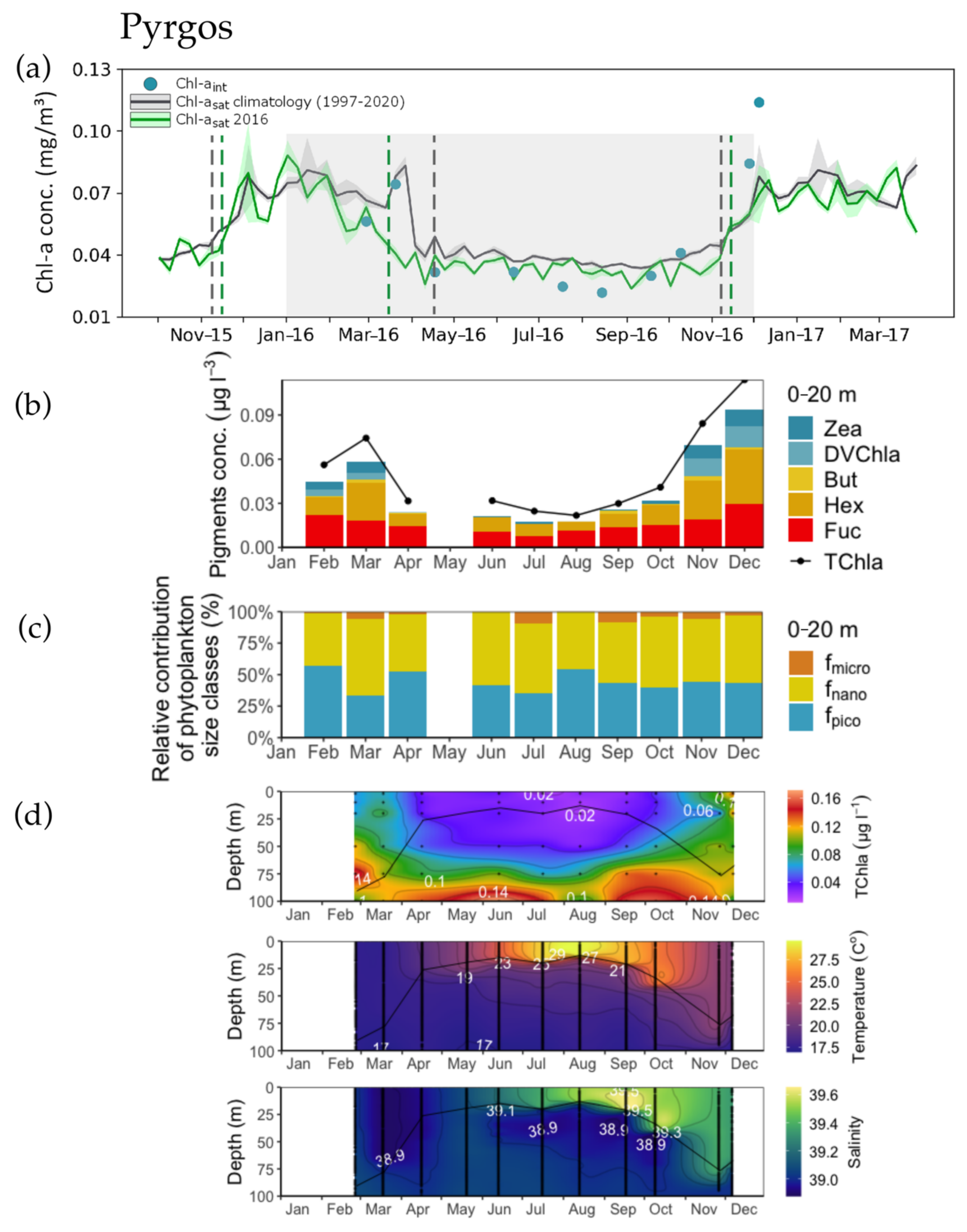
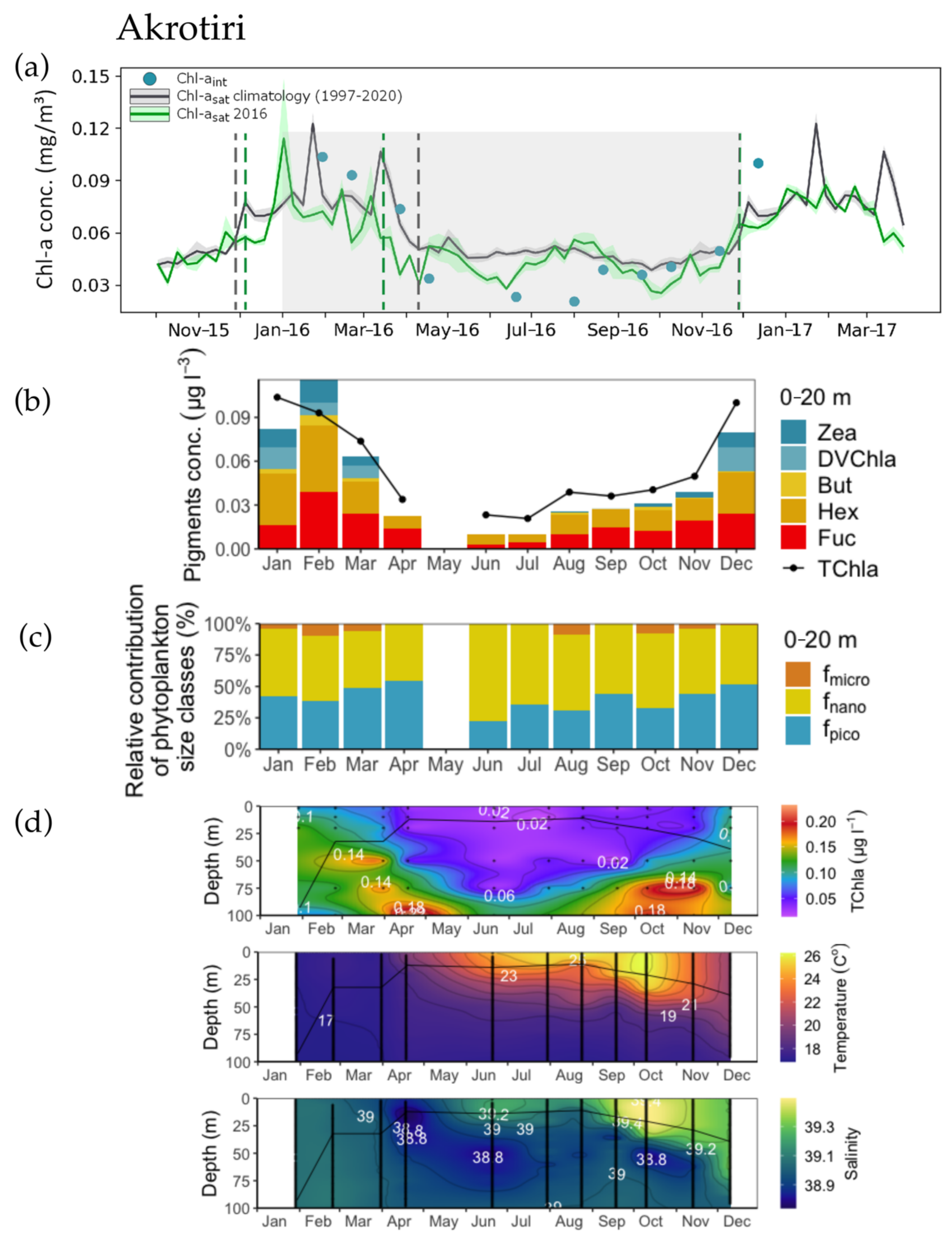
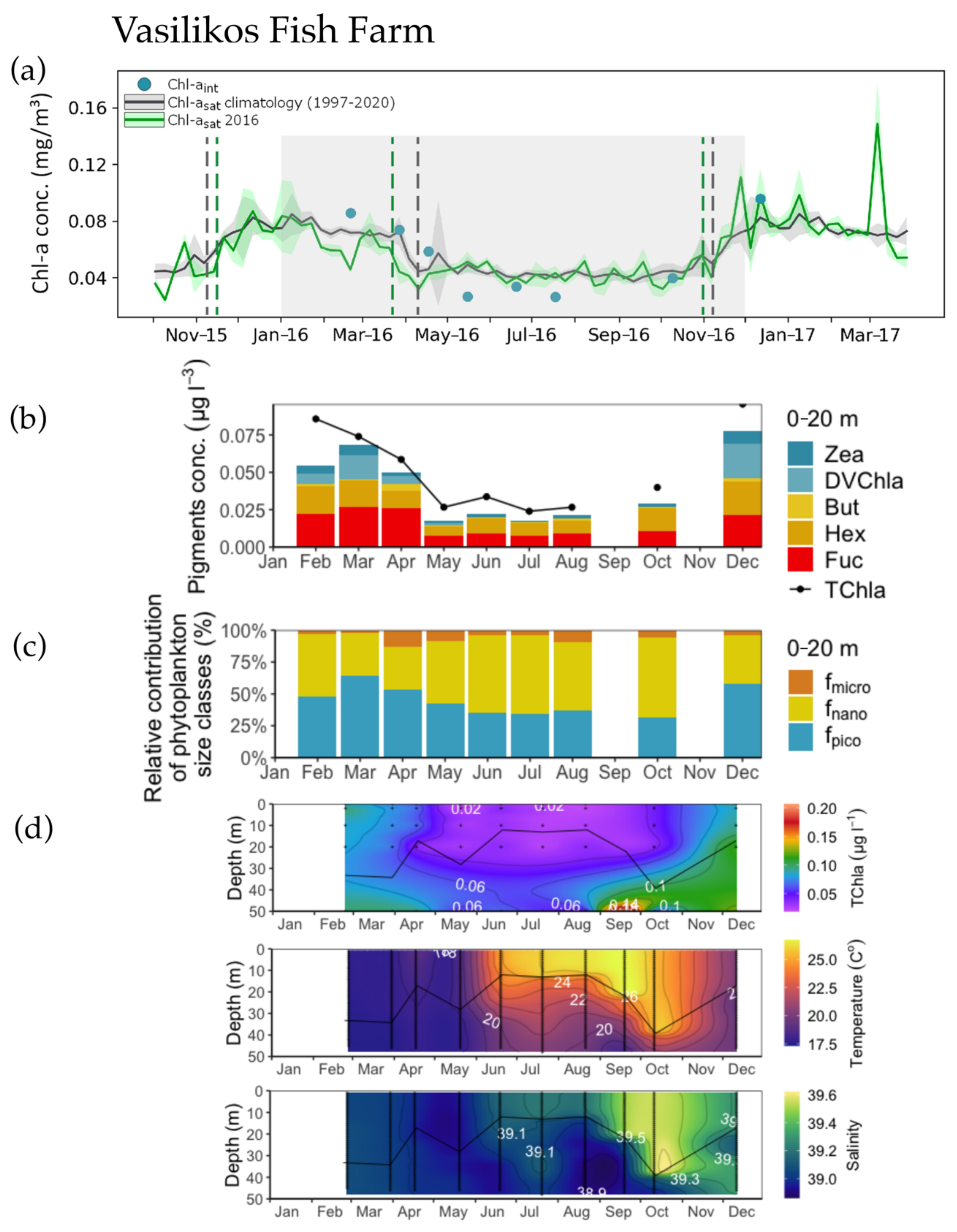
3.1. Phenology Metrics from Satellite and in situ Data Retrievals

Twenty-three years of satellite-derived Chl-a (Chl-a_sat climatology (1997–2020)) were used to compute the seasonal climatology of phytoplankton biomass and phenology. The phytoplankton growth period in the coastal waters of Cyprus initiates in early November in PYR and VAS and late November in AKR. The growth period terminates in mid-April in PYR and early April in AKR and VAS. The mean duration of the growth period lasts approximately 4 to 5 months. In 2016 (the period of in situ sampling), an earlier initiation of the growth period was observed in all stations, with PYR and VAS growth initiating in mid-November and AKR in early December. The growth period in all stations terminated in mid-March, and the growth duration was shorter by almost a month (Figure 2, Figure 3 and Figure 4).

The highest TChl-a concentration was detected in AKR, with the highest growth period occurring between January and March. The peak in PYR occurs towards the end of March. The growth period in VAS is more stable, without prominent peaks as seen in the other two stations. The results from the integrated, HPLC derived TChl-a (Chla_int, in situ data) were compared to the satellite derived values. A correlation between Chla_sat 2016 and Chla_int was observed (n = 30, ρ = 0.5, p < 0.005). The satellite and in situ data match in regard to the initiation of the main growth period, which occurs in the autumn, as well as in the timing of termination, which occurs in spring. The timing of the growth period initiation in November matches the deepening of the Mixed-Layer Depth and higher concentrations of Chl-a in the surface layers. The termination of the growth period in April coincides with a shallow MLD and low surface Chl-a concentrations.

A strong stratification was observed starting in spring and lasting until December, in all sampled stations (Figure 2, Figure 3 and Figure 4). A sharp thermocline was located at 20–50 m in PYR and AKR and at 10–40 m in VAS. Salinity was high throughout the year (>38.7), representative of the high salinity Levantine waters. The halocline followed the distribution of the thermocline in all sampled stations.

3.2. Concentration and Spatial Distribution of Phytoplankton Pigments

During the stratified period (May to November), TChl-a had a homogenous distribution in all stations (Figure 2, Figure 3 and Figure 4). The lowest TChl-a values (0.01 μg L⁻¹ in PYR and 0.02 μg L⁻¹ in AKR and VAS) were recorded in the upper layer (0–20 m), whereas the maximum values were recorded at 100 m depth in PYR (0.17 μg L⁻¹) and AKR (0.23 μg L⁻¹) and at 50 m in VAS (0.21 μg L⁻¹). Maximum concentrations of Chl-a were more prominent during spring and summer, indicating the presence of a subsurface chlorophyll maximum (SCM) layer (Figure S1).

Other diagnostic pigments typically detected in all stations were DVChl-a, Zea, But, Hex and Fuc (Table 1 for abbreviations, Figure S2). Hex (prymnesiophytes) and But (pelagophytes and chrysophytes) showed a similar distribution pattern to Chl-a. Zea (cyanobacteria) showed a decreasing trend with depth during the mixed period (January–April) in VAS station, whereas the highest values of Zea were recorded in the deepest layers in PYR during the stratified period (May–December) (Figure S3). Zea and DVChl-a had minimal concentrations during the stratified period in all stations (Figure 2, Figure 3 and Figure 4).

The dynamics of HPLC diagnostic pigments data revealed the seasonal changes in the phytoplankton community structure. TChl-a, Zea, DVChl-a, But and Fuc did not show a significantly different distribution between stations, compared to Hex, which displayed different distributions between AKR and VAS. A difference in the percentage contribution of pico- and nano-phytoplankton was also observed between AKR and VAS. Only Zea had a significantly higher concentration over the mixed period for the water column. For the 0–20 m layer, TChl-a, But and Zea had a significantly higher concentration over the mixed period. DVChl-a had a similar distribution throughout the sampling period, with almost undetectable values in the 0–20 m layer. Further, the percentage contribution of pico- and nano-phytoplankton differed between the mixed and stratified periods over the 0–20 m layer. The concentrations of TChl-a, But, Hex and Fuc varied significantly between the entire water column and the 0–20 m depth. DVChl-a and Fuc had a similar distribution between the depth layers (

Table 2. Results of one-way ANOVA tests of differences between stations, between seasons, and between depths (0–20 m, >20 m).

	Between Stations		Between Seasons				Between Depths
			Water Column		0–20 m
Variable	F	p	F	p	F	p	F	p
TChl-a	(2, 20) = 0.68		(1, 21) = 2.25		(1, 17) = 6.07	*	(1, 41) = 15.89	***
Zea	(2, 20) = 0.18		(1, 21) = 6.78	*	(1, 17) = 8.20	**	(1, 41) = 0.63
DVChl-a	(2, 20) = 1.35		(1, 21) = 0.03		(1, 9) = 0.007		(1, 33) = 3.00
But	(2, 20) = 1.30		(1, 21) = 1.42		(1, 17) = 6.02	*	(1, 41) = 10.16	**
Hex	(2, 20) = 6.81	**	(1, 21) = 0.69		(1, 17) = 2.12		(1, 41) = 19.17	***
Fuc	(2, 20) = 0.40		(1, 21) = 1.90		(1, 16) = 1.83		(1, 41) = 2.40	*
fpico	(2, 20) = 4.65	*	(1, 21) = 0.32		(1, 17) = 4.60	*	(1, 41) = 2.40
fnano	(2, 20) = 5.67	**	(1, 21) = 0.75		(1, 17) = 5.56	*	(1, 41) = 9.57	**
fmicro	(2, 20) = 1.74		(1, 21) = 1.24		(1, 17) = 0.92		(1, 41) = 0.06

p-values: 0.05 *, 0.01 **, 0.001 ***.

).

During the phytoplankton growth peak in January–February, the main pigment contribution to the TChl-a comes from Hex and Fuc, indicating a prevalence of nanophytoplankton and potentially the presence of larger cells during the peak (diatoms), even though Fuc is also found in prymnesiophytes (Figure 2b, Figure 3b and Figure 4b).

3.3. Phytoplankton Size Structure

The weighted sum of the diagnostic pigments (wDP) was linearly related to TChl-a, making DP a valid estimator of the measured TChl-a (linear regression DP = 0.6629 TChl-a +0.0023, r2 = 0.92, Figure S4). The pigment-based estimations showed that during the mixed period, f_pico accounted for about half of the depth-integrated phytoplankton biomass in the water column and the 0–20 m layer in all stations, and f_nano for the remaining half in PYR and AKR and 39% in VAS. During the stratified period, the percentage of f_nano in all stations was higher (around 60%), with f_pico accounting for approximately 40% of the depth-integrated phytoplankton biomass. The percentage of f_micro did not exceed 7% in all stations, during both the mixed and stratified periods (

Table 3. Mean (±SD) estimated contribution of pico- (f_pico), nano- (f_nano) and micro-phytoplankton (f_micro) as derived from pigment analysis, integrated over the water column and the surface layer (0–20 m), over the mixed (January–April) and stratified (May–December) periods.

			fpico (%)		fnano (%)		fmicro (%)
Station	Period	Depth	Range	Mean (±SD)	Range	Mean (±SD)	Range	Mean (±SD)
PYR	Mixed	0–20	34–52	44 ± 9	37–61	46 ± 13	2–6	3 ± 2
		0–100	38–50	44 ± 6	46–57	51 ± 6	2–5	3 ± 1
	Stratified	0–20	35–54	43 ± 6	45–59	52 ± 5	3–10	5 ± 4
		0–100	36–54	47 ± 6	42–55	48 ± 4	2–11	5 ± 3
AKR	Mixed	0–20	38–54	46 ± 7	45–54	49 ± 4	4–10	7 ± 3
		0–100	33–53	43 ± 1	45–57	51 ± 6	2–10	6 ± 4
	Stratified	0–20	22–52	37 ± 1	47–78	60 ± 10	3–8	4 ± 4
		0–100	26–57	39 ± 13	42–73	58 ± 13	1–7	3 ± 2
VAS	Mixed	0–20	48–64	55 ± 8	34–49	39 ± 9	2–13	6 ± 6
		0–50	47–64	55 ± 9	32–49	39 ± 8	4–10	6 ± 4
	Stratified	0–20	30–58	40 ± 10	38–62	54 ± 9	4–10	6 ± 3
		0–50	20–55	38 ± 13	40–73	55 ± 13	5–9	7 ± 2

).

In general, the vertical distribution of total Chl-a associated with picophytoplankton followed the distribution of Zea and DVChl a, the distribution of total Chl-a associated with nanophytoplankton followed those of Hex and But, and the total Chl-a associated with microphytoplankton was driven by the distribution pattern of Fuc (Figures S2 and S3).

The phytoplankton community was mainly dominated by picophytoplankton and nanophytoplankton, both following the distribution of TChl-a. The very low concentrations of microphytoplankton could point to the scarcity of diatoms in the study area.

4. Discussion

Long-term time series of phytoplankton phenology based both on ocean-colour remote sensing and in situ datasets can improve our understanding of phytoplankton seasonal succession. However, such a synergistic analysis for the coastal waters of Cyprus has not been carried out prior to the current study, primarily due to the lack of in situ time series on phytoplankton dynamics (on biomass and pigments). Therefore, this is the first attempt to characterise the phytoplankton dynamics in the coastal waters of Cyprus. The results from this study indicate that in situ data are consistent with the satellite-derived phytoplankton phenology in the coastal waters of Cyprus. The initiation of the phytoplankton growth period seen from the satellite in November coincides with increased concentrations of the integrated total Chl-a calculated from HPLC and with an increase in Chl-a concentrations in the surface layer. The subsurface chlorophyll maximum (SCM) in the oligotrophic Levantine is a permanent feature [55], and the increase in surface Chl-a concentration captured by the satellite in November could be attributed to the redistribution of Chl-a following the erosion of the SCM after the winter mixing, as well as to the resulting enhanced nutrient availability within the mixed layer, which triggers phytoplankton growth. The termination of the growth period in March/April co-occurs with a shallowing of the MLD, the onset of the thermocline formation which in turn limits the amount of nutrients advected to shallower depths, and the re-establishment of the SCM. The maximum values of Chl-a were recorded at 75 and 100 m depth, consistent with the SCM layer recorded in the Levantine, where the vertical distribution of Chl-a reaches maximum concentrations at around 90–110 m depth [8,56].

Based on satellite remote sensing data, the phytoplankton growth period in 2016 showed an earlier termination and thus a shorter duration compared to the Chl-a climatology (~23-year). This shorter duration of the phytoplankton growth period was also evident in the open waters of eastern Mediterranean basin in the analysis of Salgado-Hermanz et al. [39]. Various factors, global and regional, can affect the phytoplankton growth periods, leading to cascading effects in the functioning of the ecosystem, since the shifting of the growth period could alter the entire food-web structure [28]. Earlier phytoplankton growth periods could be attributed to the limited nutrients in the eastern basin, leading to very low Chl-a concentrations. Further, the El Niño Southern Oscillation index (ENSO) has been found to impact Chl-a variability in the eastern Mediterranean during its positive phase [57]. A correlation between Chl-a and nutrient-rich Saharan dust deposition has been found in the eastern Mediterranean [58], and ENSO has been found to control the export of Saharan dust in the summer [59]. Therefore, the link between Chl-a and ENSO could possibly be explained by variations in atmospheric dust deposition.

The pattern of phytoplankton growth period in the coastal waters of Cyprus shows a higher biomass between November and April and lower values in the remaining period. This pattern is in accordance to the “no bloom” classification of the oligotrophic area of the open waters of eastern Mediterranean, were a smooth rise in Chl-a concentration has been observed in October and terminates in March, with higher concentrations in fall and winter and lower values in spring and summer [60].

Since the phytoplankton size is associated with the type of waters, i.e., small-sized phytoplankton are more prominent in oligotrophic environments, and larger cells are associated with more productive waters, investigating the size structure of phytoplankton community could provide more information than the composition of the phytoplankton community itself [11]. Pigment-based estimations of the relative contribution of phytoplankton size classes can be used to determine the size distribution of phytoplankton, as an alternative to the often complicated and time-consuming various cell-counting methods (flow cytometry, inverted microscopy). Based on our HPLC pigments analysis, the pico- and nano-planktonic cells represent the most significant part of the community, consistent with oligotrophic Levantine open waters, and other Mediterranean areas where a dominance of small-sized phytoplankton by up to 80–100% of TChl-a has been recorded [7,8,11,61,62]. During the mixed season (January–April), pico- and nano-phytoplankton percentages are almost of equal importance, each one accounting for approximately 50% of the total biomass. Picophytoplankton seems to dominate slightly more in the VAS station in the southeast. This station is located next to a fish farm cage, and the increased picophytoplankton contribution to the total Chl-a is in agreement with Tsagaraki et al. [63]. During the stratified period (May–December) in southern stations AKR and VAS, the percentage of nanophytoplankton is higher, thus nanophytoplankton dominates over picophytoplankton. In general, it has been found that picoplankton dominates the eastern Mediterranean surface layers during most of the year [8,64,65], with the exception of the dynamic mesoscale structures where nanophytoplankton seems to be the dominant size class [64,66]. More specifically, when the microbial food web within and outside the Cyprus Eddy was analysed, nanoplankton were dominant followed by picoplankton and then ciliates [64]. Nanophytoplankton was also found to be dominant throughout the year in the Mediterranean, with a relative constant contribution to the total primary production [67]. Other studies carried out in the eastern Mediterranean found that the most dominant size class in the northern Levantine was picophytoplankton [68], which was also found to be dominant off the coast of Israel during the summer and fall, whereas nanoplankton were dominant during spring [6].

Akrotiri station had the highest TChl-a concentration. The southwestern coast of Cyprus, around Akrotiri peninsula, is characterized by cooler waters, most likely due to a combination of upwelling and advection from the Rhodes Gyre [69]. This coastal upwelling feature, evident during the summer, is caused by persistent westerly winds that affect the near-surface layers. The advection of cool water from the Rhodes Gyre to the southern coast of Cyprus is modelled by the Cyprus Coastal Ocean Forecasting and Observing System (CYCOFOS http://www.oceanography.ucy.ac.cy/cycofos (accessed on 7 November 2021)) [69]. The use of drifters and gliders to monitor the water masses properties of the Levantine during September 2016 and August 2017 [70] confirmed this strong upwelling during the summer months in the south of Cyprus.

The extremely low chlorophyll-a values recorded in the coastal waters of Cyprus reflect the ultraoligotrophy of the eastern Mediterranean. Eddies and currents in the area control the distribution of nutrients in the surface waters [71], whereas atmospheric depositions provide a considerable nutrient input in an otherwise nutrient-depleted area with limited input from external sources [72,73,74,75]. Even though studies conducted in the coastal waters of Turkey, north of Cyprus, recorded some of the highest total primary production values in the Mediterranean [61,68], such values are not observed in the northernmost PYR station, indicating that the exchange of productive coastal waters with oligotrophic offshore waters in the northeastern Levantine is limited.

The current study provides for the first time a complete seasonal cycle of phytoplankton phenology in the coastal waters of Cyprus, using a combination of ocean-colour remote sensing observations and analysis of in situ phytoplankton pigments. This in situ dataset is the first such dataset of phytoplankton pigments in this area, and the fact that the phenology indicators derived from the in situ Chl-a data closely match the satellite derived phenology metrics, indicates that ocean-colour remote sensing can be used to monitor and observe the marine ecosystem of Cyprus and effectively that of the eastern Levantine, where in situ observations are scarce. For instance, phytoplankton size classes (PSCs) can be derived using satellite ocean-colour observations. We anticipate that future work will entail the reparameterision of an abundance-based PSC model (e.g., [76]) with the in situ pigment dataset utilised in this study, in order to investigate variability of specific phytoplankton size classes. This approach has already been successfully applied in several oligotrophic oceanic regions such as the Red Sea [30,38,50] and the Mediterranean Sea [77]. Ultimately, this could enable a deeper understanding of how oceanic warming is affecting phytoplankton phenology and the seasonal succession of phytoplankton pigments. Considering that climate change impacts the timing of phytoplankton growth periods [25], this could alter the balance between food availability and the fitness and recruitment of higher trophic levels.

5. Conclusions

To the best of our knowledge, the present study is the first attempt to provide information on the phytoplankton seasonal succession in Cyprus, utilising a synergistic analysis of ocean-colour remote sensing and in situ data. Further, it is demonstrated that the coastal waters of Cyprus reflect the ultraoligotrophic open waters of the Levantine, as evident from the extremely low chlorophyll-a values recorded in the study area.

The overall mean duration of the phytoplankton growth period in the coastal waters of Cyprus is approximately 4 months, initiating in November and terminating in April. The higher Chl-a concentrations observed between November and April classify the coastal waters of Cyprus under the “no bloom” category of the open waters of the oligotrophic eastern Mediterranean [60]. The phytoplankton community in the coastal waters of Cyprus is dominated by pico- and nano-plankton cells. Nanophytoplakton are dominant during the growth peak in February, whereas for the rest of the year, picoplanktonic cells dominate the community, consistent with oligotrophic Levantine open waters.

The current study demonstrates the importance of ocean-colour remote sensing in regions with limited in situ datasets, such as Cyprus and the eastern Levantine. The close match observed between the in situ derived phenology indicators and the satellite derived phenology metrics, indicates the suitability of ocean-colour remote sensing in monitoring the marine ecosystem in the study area. This analysis paves the way for further investigation of the variability of specific phytoplankton size classes through the reparameterisation of an abundance-based PSC model [76], as well as for assessing the impact of oceanic warming on phytoplankton phenology. Such work will be paramount for developing a better understanding of phytoplankton dynamics and seasonal succession in the coastal waters of Cyprus, with implications for fisheries and the marine environment in general.

References

1. Azov, Y. Eastern Mediterranean—A Marine Desert? Mar. Pollut. Bull. 1991, 23, 225–232. [Google Scholar] [CrossRef]
2. Krom, M.D.; Groom, S.; Zohary, T. The Eastern Mediterranean. In Biogeochemistry of Marine Systems; Black, K.D., Shimmield, G.B., Eds.; Blackwell: Oxford, UK, 2003; p. 384. ISBN 978-1-4051-4779-8. [Google Scholar]
3. Jeffrey, S.W.; Vesk, M. Introduction to Marine Phytoplankton and Their Pigment Signatures. In Phytoplankton Pigments in Oceanography Guidlines to Modern Methods; Jeffrey, S.W., Mantoura, R.F.C., Wright, S.W., Eds.; UNESCO: Paris, France, 1997. [Google Scholar]
4. Berman, T.; Townsend, D.W.; Elsayed, S.Z.; Trees, C.C.; Azov, Y. Optical Transparency, Chlorophyll and Primary Productivity in the Eastern Mediterranean near the Israeli Coast. Oceanol. Acta 1984, 7, 367–372. [Google Scholar]
5. Berman, T.; Azov, Y.; Townsend, D. Understanding Oligotrophic Oceans: Can the Eastern Mediterranean Be a Useful Model? In Marine Phytoplankton and Productivity; Holm-Hansen, D.O., Bolis, P.L., Gilles, P.R., Eds.; Lecture Notes on Coastal and Estuarine Studies; Springer: Berlin/Heidelberg, Germany, 1984; pp. 101–112. ISBN 978-3-540-13333-9. [Google Scholar]
6. Azov, Y. Seasonal Patterns of Phytoplankton Productivity and Abundance in Nearshore Oligotrophic Waters of the Levant Basin (Mediterranean). J. Plankton Res. 1986, 8, 41–53. [Google Scholar] [CrossRef]
7. Li, W.K.W.; Zohary, T.; Yacobi, Y.Z.; Wood, A.M. Ultraphytoplankton in the Eastern Mediterranean Sea: Towards Deriving Phytoplankton Biomass from Flow Cytometric Measurements of Abundance, Fluorescence and Light Scatter. Mar. Ecol. Prog. Ser. 1993, 79–87. [Google Scholar] [CrossRef]
8. Yacobi, Y.Z.; Zohary, T.; Kress, N.; Hecht, A.; Robarts, R.D.; Waiser, M.; Wood, A.M.; Li, W.K.W. Chlorophyll Distribution throughout the Southeastern Mediterranean in Relation to the Physical Structure of the Water Mass. J. Mar. Syst. 1995, 6, 179–190. [Google Scholar] [CrossRef]
9. Psarra, S.; Tselepides, A.; Ignatiades, L. Primary Productivity in the Oligotrophic Cretan Sea (NE Mediterranean): Seasonal and Interannual Variability. Prog. Oceanogr. 2000, 46, 187–204. [Google Scholar] [CrossRef]
10. Christaki, U.; Giannakourou, A.; Van Wambeke, F.; Grégori, G. Nanoflagellate Predation on Auto- and Heterotrophic Picoplankton in the Oligotrophic Mediterranean Sea. J. Plankton Res. 2001, 23, 1297–1310. [Google Scholar] [CrossRef] [Green Version]
11. Vidussi, F.; Claustre, H.; Manca, B.B.; Luchetta, A.; Marty, J.-C. Phytoplankton Pigment Distribution in Relation to Upper Thermocline Circulation in the Eastern Mediterranean Sea during Winter. J. Geophys. Res. 2001, 106, 19939–19956. [Google Scholar] [CrossRef]
12. Petrou, A.; Kallianiotis, A.; Hannides, A.K.; Charalambidou, I.; Hadjichristoforou, M.; Hayes, D.R.; Lambridis, C.; Lambridi, V.; Loizidou, X.I.; Orfanidis, S.; et al. Initial Assessment of the Marine Environment of Cyprus: Part I - Characteristics; Ministry of Agriculture, Natural Resources, and the Environment, Department of Fisheries and Marine Research: Nicosia, Cyprus, 2012. [Google Scholar]
13. EEA EIONET Central Data Repository. Available online: http://cdr.eionet.europa.eu/cy/eea/me1/ (accessed on 7 January 2021).
14. Bianchi, T.S.; Demetropoulos, A.; Hadjichristophorou, M.; Argyrou, M.; Baskaran, M.; Lambert, C. Plant Pigments as Biomarkers of Organic Matter Sources in Sediments and Coastal Waters of Cyprus (Eastern Mediterranean). Estuar. Coast. Shelf Sci. 1996, 42, 103–115. [Google Scholar] [CrossRef] [Green Version]
15. Sofroniou, A.; Bishop, S. Water Scarcity in Cyprus: A Review and Call for Integrated Policy. Water 2014, 6, 2898–2928. [Google Scholar] [CrossRef] [Green Version]
16. WDD Water Resources—Introduction. Available online: http://www.moa.gov.cy/moa/wdd/Wdd.nsf/page08_en/page08_en?opendocument (accessed on 15 December 2020).
17. Georgiou, A. Assessment of Groundwater Resources of Cyprus; Reassessment of the island’s water resources and demand-Objective 1–Output 1.4.2; Water Development Department—Ministry of Agriculture, Rural Development and Environment: Nicosia, Cyprus, 2002; p. 234. [Google Scholar]
18. Field, C.B.; Behrenfeld, M.J.; Randerson, J.T.; Falkowski, P. Primary Production of the Biosphere: Integrating Terrestrial and Oceanic Components. Science 1998, 281, 237–240. [Google Scholar] [CrossRef] [PubMed] [Green Version]
19. Falkowski, P.G.; Raven, J.A. Aquatic Photosynthesis, 2nd ed.; Princeton University Press: Princeton, NJ, USA, 2007; ISBN 978-0-691-11550-4. [Google Scholar]
20. Reynolds, C.S. Ecology of Phytoplankton; Cambridge University Press: Cambridge, NY, USA, 2006; ISBN 978-0-511-19181-7. [Google Scholar]
21. Platt, T.; Sathyendranath, S. Ecological Indicators for the Pelagic Zone of the Ocean from Remote Sensing. Remote Sens. Environ. 2008, 112, 3426–3436. [Google Scholar] [CrossRef]
22. Edwards, M.; Richardson, A.J. Impact of Climate Change on Marine Pelagic Phenology and Trophic Mismatch. Nature 2004, 430, 881–884. [Google Scholar] [CrossRef] [PubMed]
23. Racault, M.-F.; Le Quéré, C.; Buitenhuis, E.; Sathyendranath, S.; Platt, T. Phytoplankton Phenology in the Global Ocean. Ecol. Indic. 2012, 14, 152–163. [Google Scholar] [CrossRef]
24. Racault, M.-F.; Platt, T.; Sathyendranath, S.; Airba, E.; Martinez Vicente, V.; Brewin, R. Plankton Indicators and Ocean Observing Systems: Support to the Marine Ecosystem State Assessment. J. Plankton Res. 2014, 36, 621–629. [Google Scholar] [CrossRef] [Green Version]
25. Gittings, J.A.; Raitsos, D.E.; Krokos, G.; Hoteit, I. Impacts of Warming on Phytoplankton Abundance and Phenology in a Typical Tropical Marine Ecosystem. Sci. Rep. 2018, 8, 2240. [Google Scholar] [CrossRef]
26. Robinson, C. Phytoplankton Biogeochemical Cycles. In Marine Plankton: A Pracitcal Guide to Ecology, Methodology, and Taxonomy; Oxford University Press: Oxford, UK, 2017; pp. 42–51. [Google Scholar]
27. Koeller, P.; Fuentes-Yaco, C.; Platt, T.; Sathyendranath, S.; Richards, A.; Ouellet, P.; Orr, D.; Skúladóttir, U.; Wieland, K.; Savard, L.; et al. Basin-Scale Coherence in Phenology of Shrimps and Phytoplankton in the North Atlantic Ocean. Science 2009, 324, 791–793. [Google Scholar] [CrossRef]
28. Cushing, D.H. Plankton Production and Year-Class Strength in Fish Populations: An Update of the Match/Mismatch Hypothesis. Adv. Mar. Biol. 1990, 26, 249–293. [Google Scholar] [CrossRef]
29. Platt, T.; Fuentes-Yaco, C.; Frank, K.T. Spring Algal Bloom and Larval Fish Survival. Nature 2003, 423, 398–399. [Google Scholar] [CrossRef]
30. Gittings, J.A.; Raitsos, D.E.; Brewin, R.J.W.; Hoteit, I. Links between Phenology of Large Phytoplankton and Fisheries in the Northern and Central Red Sea. Remote Sensing 2021, 13, 231. [Google Scholar] [CrossRef]
31. Wright, S.W.; Jeffrey, S.W. Pigment Markers for Phytoplankton Production. In Marine Organic Matter: Biomarkers, Isotopes and DNA; Volkman, J.K., Ed.; Springer-Verlag: Berlin/Heidelberg, Germany, 2006; Volume 2N, pp. 71–104. ISBN 978-3-540-28401-7. [Google Scholar]
32. Volpe, G.; Colella, S.; Brando, V.E.; Forneris, V.; La Padula, F.; Di Cicco, A.; Sammartino, M.; Bracaglia, M.; Artuso, F.; Santoleri, R. Mediterranean Ocean Colour Level 3 Operational Multi-Sensor Processing. Ocean Sci. 2019, 15, 127–146. [Google Scholar] [CrossRef] [Green Version]
33. Berthon, J.-F.; Zibordi, G. Bio-Optical Relationships for the Northern Adriatic Sea. Int. J. Remote Sens. 2004, 25, 1527–1532. [Google Scholar] [CrossRef]
34. D’Ortenzio, F.; Santoleri, R.; Marullo, S.; Ragni, M.; Ribera d’Alcala, M. Empirical SeaWiFS Chlorophyll Algorithm Validation for the Mediterranean Sea; Bostater, C.R., Jr., Santoleri, R., Eds.; SPIE: Barcelona, Spain, 2000; pp. 124–131. [Google Scholar]
35. Volpe, G.; Santoleri, R.; Vellucci, V.; Ribera d’Alcalà, M.; Marullo, S.; D’Ortenzio, F. The Colour of the Mediterranean Sea: Global versus Regional Bio-Optical Algorithms Evaluation and Implication for Satellite Chlorophyll Estimates. Remote Sens. Environ. 2007, 107, 625–638. [Google Scholar] [CrossRef]
36. Brewin, R.J.W.; Raitsos, D.E.; Pradhan, Y.; Hoteit, I. Comparison of Chlorophyll in the Red Sea Derived from MODIS-Aqua and in Vivo Fluorescence. Remote Sens. Environ. 2013, 136, 218–224. [Google Scholar] [CrossRef]
37. Racault, M.-F.; Raitsos, D.E.; Berumen, M.L.; Brewin, R.J.W.; Platt, T.; Sathyendranath, S.; Hoteit, I. Phytoplankton Phenology Indices in Coral Reef Ecosystems: Application to Ocean-Color Observations in the Red Sea. Remote Sens. Environ. 2015, 160, 222–234. [Google Scholar] [CrossRef] [Green Version]
38. Gittings, J.A.; Raitsos, D.E.; Kheireddine, M.; Racault, M.-F.; Claustre, H.; Hoteit, I. Evaluating Tropical Phytoplankton Phenology Metrics Using Contemporary Tools. Sci. Rep. 2019, 9, 674. [Google Scholar] [CrossRef]
39. Salgado-Hernanz, P.M.; Racault, M.-F.; Font-Muñoz, J.S.; Basterretxea, G. Trends in Phytoplankton Phenology in the Mediterranean Sea Based on Ocean-Colour Remote Sensing. Remote Sens. Environ. 2019, 221, 50–64. [Google Scholar] [CrossRef]
40. Van Heukelem, L.; Thomas, C.S. Computer-Assisted High-Performance Liquid Chromatography Method Development with Applications to the Isolation and Analysis of Phytoplankton Pigments. J. Chromatogr. A 2001, 910, 31–49. [Google Scholar] [CrossRef]
41. Lagaria, A.; Mandalakis, M.; Mara, P.; Frangoulis, C.; Karatsolis, B.-T.; Pitta, P.; Triantaphyllou, M.; Tsiola, A.; Psarra, S. Phytoplankton Variability and Community Structure in Relation to Hydrographic Features in the NE Aegean Frontal Area (NE Mediterranean Sea). Cont. Shelf Res. 2017, 149, 124–137. [Google Scholar] [CrossRef]
42. Mandalakis, M.; Stravinskaitė, A.; Lagaria, A.; Psarra, S.; Polymenakou, P. Ultrasensitive and High-Throughput Analysis of Chlorophyll a in Marine Phytoplankton Extracts Using a Fluorescence Microplate Reader. Anal. Bioanal. Chem. 2017, 409, 4539–4549. [Google Scholar] [CrossRef]
43. Laws, E.A. Mathematical Methods for Oceanographers: An Introduction; Wiley: New York, NY, USA, 1997; ISBN 978-0-471-16221-6. [Google Scholar]
44. Al-Naimi, N.; Raitsos, D.E.; Ben-Hamadou, R.; Soliman, Y. Evaluation of Satellite Retrievals of Chlorophyll-a in the Arabian Gulf. Remote Sens. 2017, 9, 301. [Google Scholar] [CrossRef] [Green Version]
45. De Boyer Montégut, C. Mixed Layer Depth over the Global Ocean: An Examination of Profile Data and a Profile-Based Climatology. J. Geophys. Res. 2004, 109, C12003. [Google Scholar] [CrossRef]
46. Amante, C.; Eakins, B.W. ETOPO1 1 Arc-Minute Global Relief Model: Procedures, Data Sources and Analysis; National Geophysical Data Center: Boulder, CO, USA, 2009. [Google Scholar]
47. Amante, C.; Eakins, B.W. ETOPO1 1 Arc-Minute Global Relief Model; NOAA National Geophysical Data Center: Boulder, CO, USA, 2009. [Google Scholar]
48. Uitz, J.; Claustre, H.; Morel, A.; Hooker, S.B. Vertical Distribution of Phytoplankton Communities in Open Ocean: An Assessment Based on Surface Chlorophyll. J. Geophys. Res. 2006, 111, C08005. [Google Scholar] [CrossRef]
49. Gittings, J.A.; Brewin, R.J.W.; Raitsos, D.E.; Kheireddine, M.; Ouhssain, M.; Jones, B.H.; Hoteit, I. Remotely Sensing Phytoplankton Size Structure in the Red Sea. Remote Sens. Environ. 2019, 234, 111387. [Google Scholar] [CrossRef]
50. Brewin, R.J.W.; Morán, X.A.G.; Raitsos, D.E.; Gittings, J.A.; Calleja, M.L.; Viegas, M.; Ansari, M.I.; Al-Otaibi, N.; Huete-Stauffer, T.M.; Hoteit, I. Factors Regulating the Relationship Between Total and Size-Fractionated Chlorophyll-a in Coastal Waters of the Red Sea. Front. Microbiol. 2019, 10, 1964. [Google Scholar] [CrossRef] [PubMed]
51. Jeffrey, S.W.; Wright, S.W.; Zapata, M. Microalgal Classes and Their Signature Pigments. In Phytoplankton Pigments: Characterization, Chemotaxonomy, and Applications in Oceanography; Cambridge University Press: Cambridge, NY, USA, 2011; ISBN 978-1-107-00066-7. [Google Scholar]
52. R Core Team. R: A Language and Environment for Statistical Computing; R Foundation for Statistical Computing: Vienna, Austria, 2021. [Google Scholar]
53. Finley, A.; Banerjee, S.; Hjelle, Ø. MBA: Multilevel B-Spline Approximation; CRAN, 2017. [Google Scholar]
54. Wickham, H. Ggplot2: Elegant Graphics for Data Analysis, 2nd ed.; Springer: New York, NY, USA, 2016; ISBN 978-3-319-24277-4. [Google Scholar]
55. Barbieux, M.; Uitz, J.; Gentili, B.; Pasqueron de Fommervault, O.; Mignot, A.; Poteau, A.; Schmechtig, C.; Taillandier, V.; Leymarie, E.; Penkerc’h, C.; et al. Bio-Optical Characterization of Subsurface Chlorophyll Maxima in the Mediterranean Sea from a Biogeochemical-Argo Float Database. Biogeosciences 2019, 16, 1321–1342. [Google Scholar] [CrossRef] [Green Version]
56. Krom, M.D.; Thingstad, T.F.; Brenner, S.; Carbo, P.; Drakopoulos, P.; Fileman, T.W.; Flaten, G.A.F.; Groom, S.; Herut, B.; Kitidis, V.; et al. Summary and Overview of the CYCLOPS P Addition Lagrangian Experiment in the Eastern Mediterranean. Deep Sea Res. Part II Top. Stud. Oceanogr. 2005, 52, 3090–3108. [Google Scholar] [CrossRef]
57. Salgado-Hernanz, P.M. Patterns of Phytoplankton and Primary Production Variability in the Mediterranean Sea Based on Remote Sensing Data. Ph.D. Thesis, Universitat de les Illes Balears, Palma, Spain, 2019. [Google Scholar]
58. Gallisai, R.; Peters, F.; Volpe, G.; Basart, S.; Baldasano, J.M. Saharan Dust Deposition May Affect Phytoplankton Growth in the Mediterranean Sea at Ecological Time Scales. PLoS ONE 2014, 9, e110762. [Google Scholar] [CrossRef] [Green Version]
59. Deflorio, M.; Aprea, A.; Corriero, A.; Santamaria, N.; De Metrio, G. Incidental Captures of Sea Turtles by Swordfish and Albacore Longlines in the Ionian Sea. Fish. Sci. 2005, 71, 1010–1018. [Google Scholar] [CrossRef]
60. D’Ortenzio, F.; Ribera d’Alcalà, M. On the Trophic Regimes of the Mediterranean Sea: A Satellite Analysis. Biogeosciences 2009, 6, 139–148. [Google Scholar] [CrossRef] [Green Version]
61. Yücel, N. Monthly Changes in Primary and Bacterial Productivity in the North-Eastern Mediterranean Shelf Waters. Ph.D. Thesis, Middle East Technical University, Ankara, Turkey, 2013. [Google Scholar]
62. Siokou-Frangou, I.; Christaki, U.; Mazzocchi, M.G.; Montresor, M.; Ribera d’Alcalá, M.; Vaqué, D.; Zingone, A. Plankton in the Open Mediterranean Sea: A Review. Biogeosciences 2010, 7, 1543–1586. [Google Scholar] [CrossRef] [Green Version]
63. Tsagaraki, T.; Pitta, P.; Frangoulis, C.; Petihakis, G.; Karakassis, I. Plankton Response to Nutrient Enrichment Is Maximized at Intermediate Distances from Fish Farms. Mar. Ecol. Prog. Ser. 2013, 493, 31–42. [Google Scholar] [CrossRef] [Green Version]
64. Tanaka, T.; Zohary, T.; Krom, M.D.; Law, C.S.; Pitta, P.; Psarra, S.; Rassoulzadegan, F.; Thingstad, T.F.; Tselepides, A.; Woodward, E.M.S.; et al. Microbial Community Structure and Function in the Levantine Basin of the Eastern Mediterranean. Deep Sea Res. Part I Oceanogr. Res. Pap. 2007, 54, 1721–1743. [Google Scholar] [CrossRef]
65. Zohary, T.; Brenner, S.; Krom, M.; Angel, D.; Kress, N.; Li, W.; Neori, A.; Yacobi, Y. Buildup of Microbial Biomass during Deep Winter Mixing in a Mediterranean Warm-Core Eddy. Mar. Ecol. Prog. Ser. 1998, 167, 47–57. [Google Scholar] [CrossRef]
66. Psarra, S.; Zohary, T.; Krom, M.D.; Mantoura, R.F.C.; Polychronaki, T.; Stambler, N.; Tanaka, T.; Tselepides, A.; Frede Thingstad, T. Phytoplankton Response to a Lagrangian Phosphate Addition in the Levantine Sea (Eastern Mediterranean). Deep Sea Res. Part II Top. Stud. Oceanogr. 2005, 52, 2944–2960. [Google Scholar] [CrossRef]
67. Uitz, J.; Stramski, D.; Gentili, B.; D’Ortenzio, F.; Claustre, H. Estimates of Phytoplankton Class-Specific and Total Primary Production in the Mediterranean Sea from Satellite Ocean Color Observations. Global Biogeochem. Cycles 2012, 26, GB2024. [Google Scholar] [CrossRef]
68. Yücel, N. Spatio-Temporal Variability of the Size-Fractionated Primary Production and Chlorophyll in the Levantine Basin (Northeastern Mediterranean). Oceanologia 2018, 60, 288–304. [Google Scholar] [CrossRef]
69. Zodiatis, G.; Lardner, R.; Hayes, D.R.; Georgiou, G.; Sofianos, S.; Skliris, N.; Lascaratos, A. Operational Ocean Forecasting in the Eastern Mediterranean: Implementation and Evaluation. Ocean Sci. 2008, 4. [Google Scholar] [CrossRef] [Green Version]
70. Mauri, E.; Lardner, R.; Sitz, L.; Gerin, R.; Poulain, P.-M.; Hayes, D.; Gildor, H. On the Variability of the Circulation and Water Mass Properties in the Eastern Levantine Sea between September 2016–August 2017. Water 2019, 11, 1741. [Google Scholar] [CrossRef] [Green Version]
71. Ediger, D.; Yilmaz, A. Characteristics of Deep Chlorphyll Maximum in the Northeastern Mediterranean with Respect to Environmental Conditions. J. Mar. Syst. 1996, 9, 291–303. [Google Scholar] [CrossRef]
72. Krom, M.D.; Herut, B.; Mantoura, R.F.C. Nutrient Budget for the Eastern Mediterranean: Implications for Phosphorus Limitation. Limnol. Oceanogr. 2004, 49, 1582–1592. [Google Scholar] [CrossRef]
73. Herut, B.; Zohary, T.; Krom, M.D.; Mantoura, R.F.C.; Pitta, P.; Psarra, S.; Rassoulzadegan, F.; Tanaka, T.; Frede Thingstad, T. Response of East Mediterranean Surface Water to Saharan Dust: On-Board Microcosm Experiment and Field Observations. Deep Sea Research Part II: Topical Studies in Oceanography 2005, 52, 3024–3040. [Google Scholar] [CrossRef]
74. Markaki, Z.; Oikonomou, K.; Kocak, M.; Kouvarakis, G.; Chaniotaki, A.; Kubilay, N.; Mihalopoulos, N. Atmospheric Deposition of Inorganic Phosphorus in the Levantine Basin, Eastern Mediterranean: Spatial and Temporal Variability and Its Role in Seawater Productivity. Limnol. Oceanogr. 2003, 48, 1557–1568. [Google Scholar] [CrossRef] [Green Version]
75. Markaki, Z.; Loÿe-Pilot, M.D.; Violaki, K.; Benyahya, L.; Mihalopoulos, N. Variability of Atmospheric Deposition of Dissolved Nitrogen and Phosphorus in the Mediterranean and Possible Link to the Anomalous Seawater N/P Ratio. Mar. Chem. 2010, 120, 187–194. [Google Scholar] [CrossRef]
76. Brewin, R.J.W.; Sathyendranath, S.; Hirata, T.; Lavender, S.J.; Barciela, R.M.; Hardman-Mountford, N.J. A Three-Component Model of Phytoplankton Size Class for the Atlantic Ocean. Ecol. Model. 2010, 221, 1472–1483. [Google Scholar] [CrossRef]
77. Sammartino, M.; Di Cicco, A.; Marullo, S.; Santoleri, R. Spatio-Temporal Variability of Micro-, Nano- and Pico-Phytoplankton in the Mediterranean Sea from Satellite Ocean Colour Data of SeaWiFS. Ocean Sci. 2015, 11, 759–778. [Google Scholar] [CrossRef] [Green Version]
Figure 1. Bathymetry map around Cyprus at the eastern Mediterranean Sea, indicating the three sampling stations, Pyrgos (PYR), Akrotiri (AKR) and Vasilikos Fish Farm (VAS). Bathymetric data obtained from the National Geophysical Data Centre (NGDC) database ETOPO1 [46,47], and coastline data obtained from naturalearthdata.com.
Remotesensing 14 00012 g001
Figure 2. Time series of satellite-derived Chl-a consecrations, diagnostic pigment concentrations and vertical profiles of total Chl-a, temperature and salinity in Pyrgos (PYR) station. (a) Climatology time-series (based on 23-year OC-CNR data of daily composites) (Chl-asat climatology (1997–2020) in comparison with satellite-derived Chl-a concentration from October 2015 to March 2017 (Chl-asat 2016). Blue dots represent the in situ measurements (Chl-aint) taken between January and December 2016 (shaded area). The dashed lines represent the timing of initiation and termination of the main phytoplankton growth, (b) Diagnostic pigments concentrations for the 0–20 m layer, (c) Percentages associated with the pico- (fpico), nano- (fnano) and micro-phytoplankton (fmicro) size classes, for the 0–20 m layer, (d) Vertical profiles of CTD temperature, salinity, and HPLC total Chl-a concentration. The black line represents the Mixed-Layer Depth (MLD). Note: The in situ data are a snapshot (one day in each month) compared to the weekly averages of the satellite retrieved data.
Remotesensing 14 00012 g002
Figure 3. Time series of satellite-derived Chl-a consecrations, diagnostic pigment concentrations and vertical profiles of total Chl-a, temperature, and salinity in Akrotiri (AKR) station. (a) Climatology time-series (based on 23-year OC-CNR data of daily composites) (Chl-asat climatology (1997–2020) in comparison with satellite-derived Chl-a concentration from October 2015 to March 2017 (Chl-asat 2016). Blue dots represent the in situ measurements (Chl-aint) taken between January and December 2016 (shaded area). The dashed lines represent the timing of initiation and termination of the main phytoplankton growth, (b) Diagnostic pigments concentrations for the 0–20 m layer, (c) Percentages associated with the pico- (fpico), nano- (fnano) and micro-phytoplankton (fmicro) size classes, for the 0–20 m layer, (d) Vertical profiles of CTD temperature, salinity, and HPLC total Chl-a concentration. The black line represents the Mixed-Layer Depth (MLD). Note: The in situ data are a snapshot (one day in each month) compared to the weekly averages of the satellite retrieved data.
Remotesensing 14 00012 g003
Figure 4. Time series of satellite-derived Chl-a consecrations, diagnostic pigment concentrations and vertical profiles of total Chl-a, temperature, and salinity in Vasilikos Fish Farm (VAS) station. (a) Climatology time-series (based on 23-year OC-CNR data of daily composites) (Chl-asat climatology (1997–2020) in comparison with satellite-derived Chl-a concentration from October 2015 to March 2017 (Chl-asat 2016). Blue dots represent the in situ measurements (Chl-aint) taken between January and December 2016 (shaded area). The dashed lines represent the timing of initiation and termination of the main phytoplankton growth, (b) Diagnostic pigments concentrations for the 0–20 m layer, (c) Percentages associated with the pico- (fpico), nano- (fnano) and micro-phytoplankton (fmicro) size classes, for the 0–20 m layer, (d) Vertical profiles of CTD temperature, salinity, and HPLC total Chl-a concentration. The black line represents the Mixed-Layer Depth (MLD). Note: The in situ data are a snapshot (one day in each month) compared to the weekly averages of the satellite retrieved data.
Remotesensing 14 00012 g004