Temporal Variability of Oceanic Mesoscale Events in the Gulf of California

Abstract

Oceanic mesoscale events such as eddies, coastal upwelling, filaments and fronts created by water mass intrusion present properties allowing them to concentrate, transport and disperse salt, nutrients and plankton, among other important constituents in the ocean. The use of satellite images enables the continuous monitoring of the ocean dynamics at different temporal and spatial scales, aiding the study of its variability. This study focuses on the identification of these mesoscale events in the Gulf of California (GC) by means of sea surface temperature (SST) and chlorophyll a (Chl a) fronts (edge) detection by processing 5-day satellite images from the 1998–2019 period. The annual occurrence or frequency and duration of each event was identified; the interannual variability was evaluated and underlying correlations with the Multivariate El Niño Index (MEI) and the Pacific Decadal Index (PDOI) were assessed via Principal Component Analysis. Most events showed a seasonal variability due to the seasonal behavior of forcing agents (i.e., Pacific Ocean and winds) that stimulate their formation or presence in the GC; seasonality was more evident in the northern region than in the southern region. The interannual variability of their frequency or duration was associated with strong and intense El Niño and La Niña conditions (positive or negative MEI values) together with positive or negative phases of the PDOI. The use of SST and Chl a satellite images with a 5-day temporal resolution allowed to better identify and quantify the annual frequency and duration of each mesoscale event. It allowed to detect a seasonal behavior of these events in the northern region, followed by the central region. The southern region, due to the interaction of different water masses with unique characteristics, exhibited a less evident seasonality in the frequency of eddies, and no apparent association between their interannual frequency and duration with the MEI and PDOI. Constantly monitoring these oceanic events and their variability will help in the understanding of how the different regions of this large marine ecosystem respond to these variations in the long term.

1. Introduction

Physical events in the marine environment may generate structures at various spatial and temporal scales so they are important in delimiting sea surface temperature (SST) gradients in extensive oceanic regions of the world. These structures include mesoscale events exhibiting dimensions raging from tens to a few hundred kilometers and a life span from several weeks to a few months [1,2]. Structures, such as mesoscale eddies that are often referred to as the ocean “weather”, include vortices distinguished by temperature and salinity anomalies; they possess distinctive properties allowing them to transport heat, salt, carbon and nutrients [3]. They can be generated by barotropic or baroclinic instabilities, by atmospheric forcing, and by the interaction between water mass movements with irregular continental shelves, with islands or capes [4,5]. As a classic conception, in the Northern Hemisphere cyclonic eddies have counterclockwise rotation that displays cold cores as a consequence of a sheer mixed layer and rise of the thermocline, while anticyclonic eddies with clockwise rotation possess warmer cores [6,7]. However, this conception has been questioned, as it has been shown that anticyclonic eddies can be equally or more productive than the cyclonic ones, due to weaker stratification during summer in anticyclonic than in cyclonic eddies [8]. Furthermore, eddy decay time scale, eddy amplitude and eddy radius scale play an important role in the magnitude of eddy pumping [9]. Additionally, Wang et al. [10] concluded that the effects of mesoscale eddy on pigment concentration are dependent on the distances with the eddy core, as anticyclonic eddies can exhibit higher chlorophyll within the transition zone of an eddy. Analyzing and processing satellite images with specialized techniques allows a synoptic view of the distribution, temporal and spatial variability of eddies, upwelling events, and filaments in regions with high occurrence; these areas are generally under the influence of important marine current systems [4,11,12].

One of these areas is the Gulf of California (GC) where its geographic location, bathymetry, topography and climate contribute to processes dominated by atmospheric and oceanic forcing [13], which are decisive in the SST seasonal and interannual behavior. Furthermore, the interaction of atmospheric and oceanic forcing with the coast and bathymetry promotes the formation of oceanic mesoscale events (OME), such as mesoscale eddies, coastal upwelling, and filaments in different regions of the GC [14,15]. García-Morales et al. [14] and Robles-Tamayo et al. [16] identified seasonal, annual and interannual SST variability in the eastern coast of the GC related to OME and to large-scale ocean–atmosphere interactions (i.e., El Niño and La Niña events).

The GC is one of the most diverse regions in the world [17,18] where numerous important fisheries take place, including forage fish (e.g., Pacific sardine, thread herring, northern anchovy, Pacific mackerel), all of them important species for maintaining multiple food chains [19,20]. These forage fish species are distributed along the GC and are greatly dependent on areas with high productivity, food availability and optimal SST [21]. Eddies are highly dynamic and based on their physical characteristics, different processes may influence the horizontal [22] and the vertical [23] water exchange. These processes can promote the transport of nutrients between the euphotic and deeper layer, aiding the growth of phytoplankton and influencing the distribution of surface chlorophyll [10]. Moreover, mesoscale hydrographic structure and eddies dynamics, and their possible interactions with surrounding coastal processes, may contribute towards the existence of different spatial and vertical habitats affecting the vertical and horizontal distribution of fish larvae [24]. Furthermore, the vertical structure of eddies may contain distinct water masses that can be dominated by different species, representing habitats for larvae [25]. Due to the importance of OME (e.g., eddies and upwelling) on local SST and chlorophyll a (Chl a) variations, their variability can be a determining factor in the dynamics of several regions in the GC, either aiding or hindering enrichment, concentration and dispersion of planktonic and meroplanktonic organisms with effects on recruitment, distribution and abundance of important fishery resources [19,25]. Thus, the study of temporal and spatial variability of these mesoscale structures is desirable.

In Eastern Boundary Current Systems and particularly in the California Current System, the SST fronts distribution is characterized by seasonal variability [26], which is influenced by upwelling mesoscale dynamics [27] and wind forcing [28]. The interannual variability of these fronts’ probability is influenced by the ENSO. Under positive ENSO (El Niño) conditions, propagation towards the east of equatorial Kelvin waves deepens the thermocline, reducing SST gradients and affecting the probability of fronts in the Eastern Pacific [29]. Furthermore, under positive ENSO conditions there are negative anomalies of frontal activity in regions where wind stress convergence takes place; the opposite is observed under La Niña conditions, when higher frontal probability occurs [29]. These scenarios could also apply to eddy activity, as they are important in the generation of SST and Chl a fronts, relevant in the mesoscale dynamics of the GC. The dynamics of eddies and fronts are closely related [30], hence, the objective of this study was to evaluate the annual occurrence and interannual variability of OME, contributing to the comprehension of the high environmental variability and species diversity of the Gulf of California. This study uses SST and Chl a satellite images with 5-day temporal resolution and 1 km spatial resolution to better identify and quantify the frequency and duration of each OME in the GC; in addition, the 22-year analyses allow a better estimation of their variability and its possible relation with large-scale climatic events such as El Niño (EN), La Niña (LN) and the Pacific Decadal Oscillation (PDO).

2. Materials and Methods

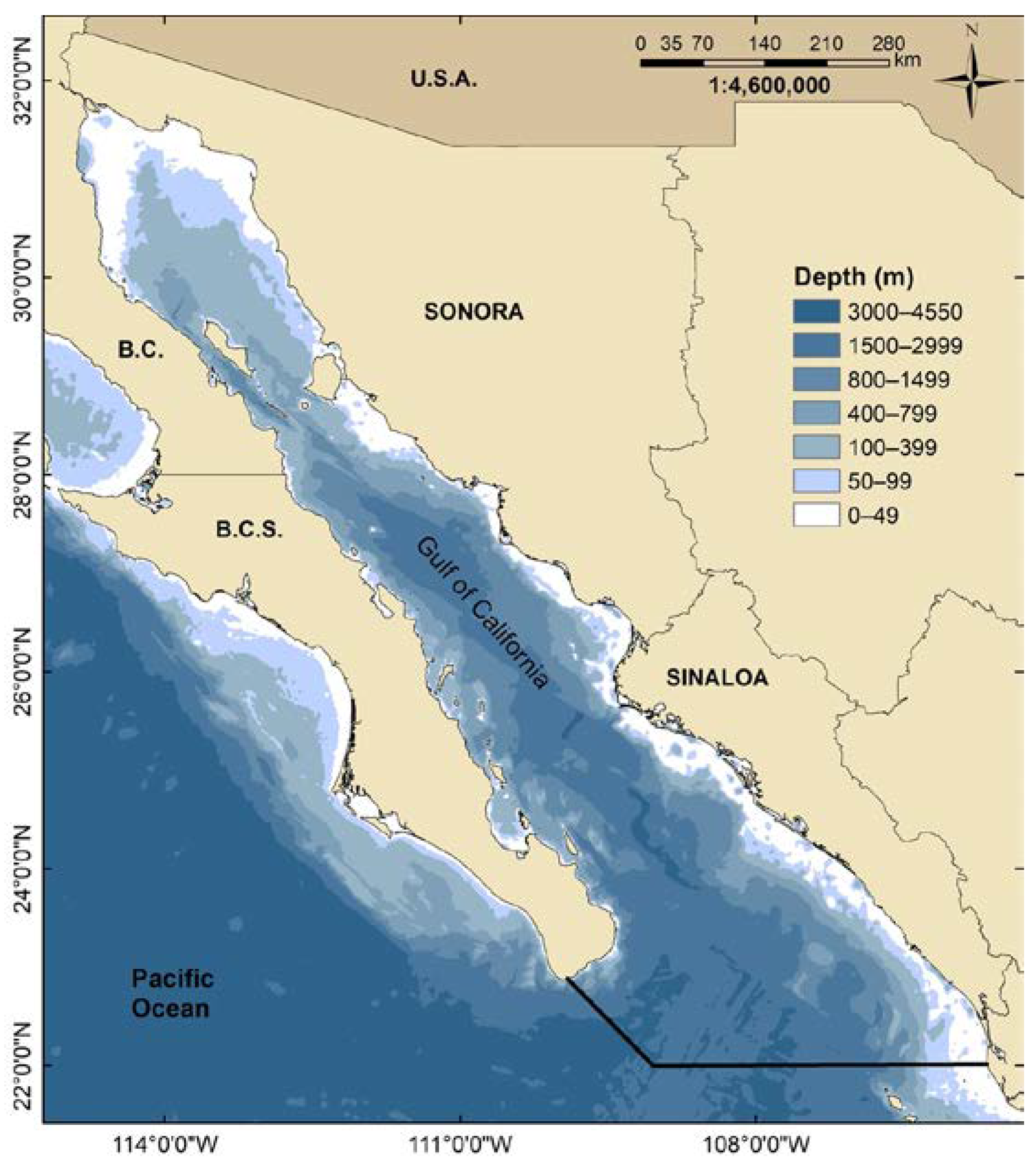
2.1. Study Area

The Gulf of California is a semi-closed sea surrounded almost entirely by topographic elevations and has direct communication with the Pacific Ocean (PO) at its southern end [31]. It is located in the temperate–tropical transition zone, so it has a complex climate, oceanographic and ecological characteristics [32]. The general circulation in the GC is determined by the PO, wind stress, air–sea heat fluxes [33,34,35]. The thermohaline circulation is also important, particularly in the southern region which is a convergence zone where Tropical Surface Water, California Current Water and Gulf of California water interact, displaying a complex thermohaline structure generator of fronts that develop structures such as eddies, meander and jets visible in satellite images [36,37]. The study area cover 31°30′N, 114°48′W to 22°00′N, 105°40′W (Figure 1).

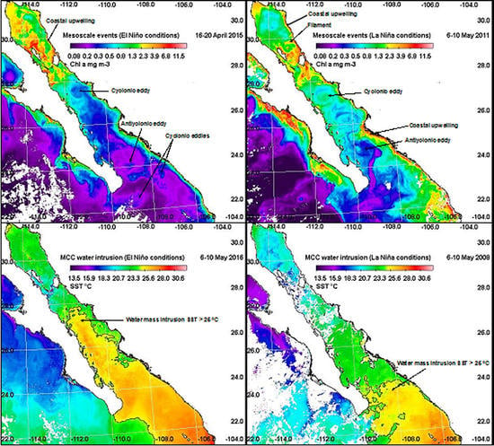
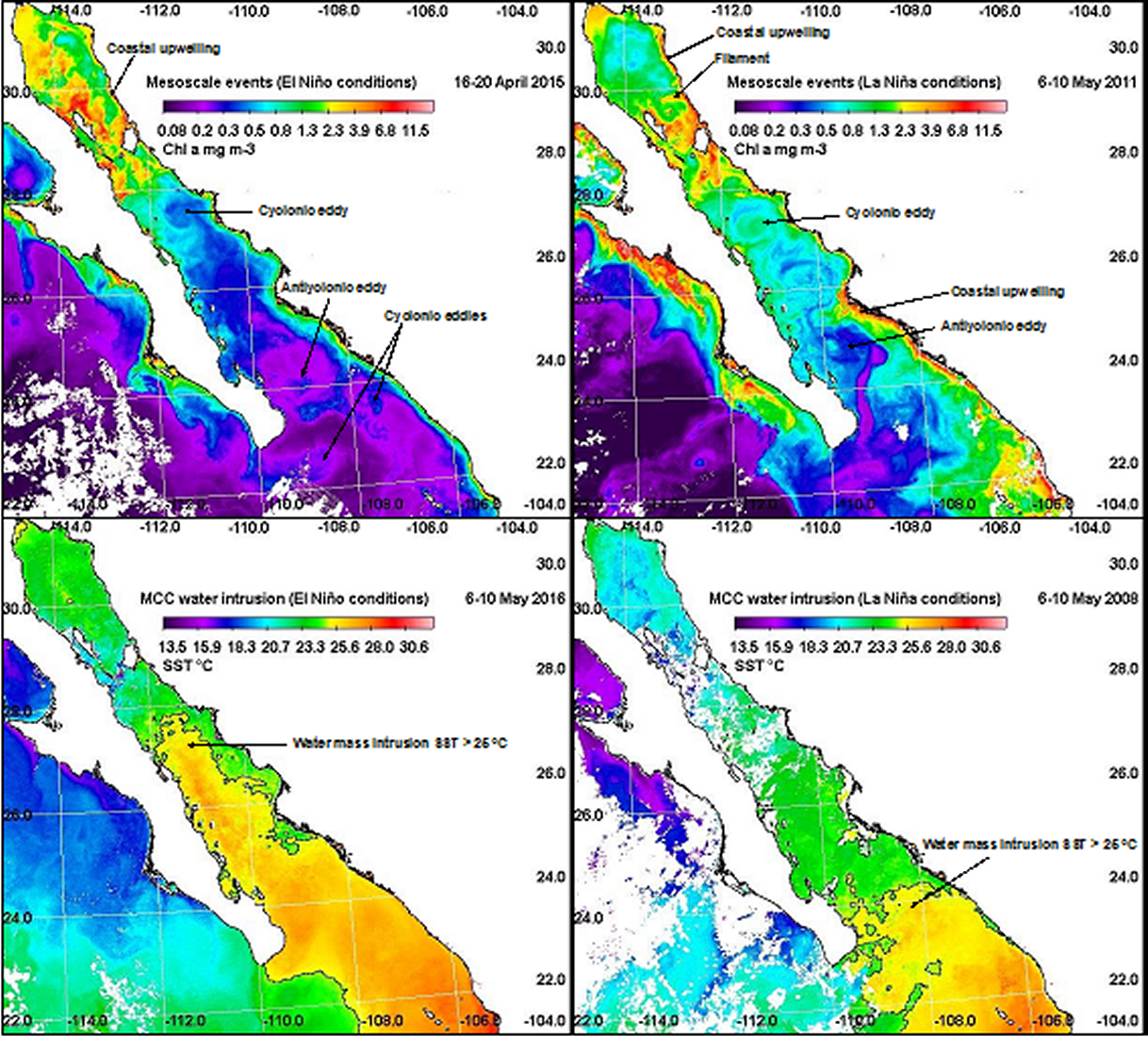
2.2. Oceanic Mesoscale Events

For the OME analyses, a composite of 1 km resolution, 5-day SST satellite images from MODIS Terra/Aqua and VIIRS sensors, and 5-day, 1 km resolution Chl a satellite images from the SeaWiFS, MODIS Aqua/Terra, MERIS, VIIRS and OLCI sensors were used, all available at http://www.wimsoft.com/CAL/ (accessed on 26 January 2020). The use of 5-day temporal resolution gave more precise estimations of each OME duration; in addition, it made the detection of SST and Chl a gradients and fronts required for the OME identification suitable. Image processing and analyses were carried out using routines from Windows Image Manager Software (WIM version 9.06; 1991–2015, Copyright^® Mati Kahru, San Diego, CA, USA; wim@wamsoft.com).

Considering that mesoscale events can occur at a timescale of several weeks to several months [38] and at a spatial scale of tens to hundreds of kilometers [30], in our study we only included eddies with a lifespan longer than 15 days. Additionally, several studies have documented the existence of mesoscale eddies with a defined vertical structure in the GC. Carrillo et al. [39], by estimating the geostrophic circulation in the northern Gulf of California, identified well-defined features of 100 m in depth. Furthermore, summer eddies of 2004 observed in satellite images [15] have been validated by Castro et al. [40] through direct hydrographic observations, finding that the subsurface (<20 m) thermohaline structure and circulation pattern were dominated by mesoscale eddies which were mostly geostrophic and with depths of 900 m.

Hence, eddies were identified by applying criteria from previous studies of Pegau et al. [40,41] and García-Morales et al. [14]. Furthermore, Kahru et al. [6,7] method was followed, where the edge detection method Cayula and Cornillon [42] was applied by means of the Single Image Edge Detection (SIED) subroutine from WIMSoft^®, San Diego, CA, USA. This method uses overlapping windows to explore the statistical probability of an edge; first, it calculates and discriminated the bimodality of the histogram; then, it detects the cohesion of the potential edge; finally, it applies a modification proposed by Diehl et al. [43], which employs a two-way variogram analysis to find the best window size in horizontal and vertical directions instead of a fixed window size. Edges were detected in both Chl a and SST 5-day satellite images to determine the type of eddy depending on the core temperature, which is cyclonic according to Cruz Gómez et al. [5] if the core is relatively cooler than its edge, while it is anticyclonic if the core is relatively warmer than its edge.

Most satellite altimetry products (sea level anomaly) have a spatial resolution of 0.25 degrees longitude/latitude, making difficult the use of these products for eddy detection in the Gulf of California which has an average spatial extent of ~150 km in zonal direction. However, global ocean eddy resolving models from the GLORYS12V1 product (CMEMS) from the Copernicus Marine Service ocean products available at https://resources.marine.copernicus.eu (accessed on 2 February 2021) aided the validation of eddies identified in our study.

Following similar previous methods, García-Reyes et al. [44] and Dabuleviciene et al. [45] identified, in different marine areas, coastal upwelling events along the east coast of the GC using a 1° C threshold between coastal and offshore water at the same latitude in the 5-day SST satellite images. Additionally, SST and Chl a edge detection was applied to the satellite images using the SIED subroutine, based on the assumption that both types of fronts should agree, meaning that cold nutrient-rich sub-surface water has been upwelled.

The filaments analyzed in this study are the ones resulting from coastal upwelling, therefore, filaments are elongated narrow structures with distinctive temperature and salinity, winds being their forcing agent, which associates the upwelling season with filament formation [46,47]. They are biologically important structures as they transport coastal waters with high Chl a concentration to the offshore [47,48]. These structures were detected first by transforming the Chl a values to square power to highlight the eutrophic (<1 mg m⁻³) areas in the satellite images; afterwards, longitudinal and latitudinal projections originated from coastal upwelling areas were identified via the SIED subroutine. Filaments were discerned from river-derived plumes because the former display colder SST compared to their surroundings, as a consequence of coastal upwelling, while the latter, according to Martínez Flores et al. [49], have warmer SST compared to the surrounding water, and can be detectable in the 5-day satellite images.

Warm oligotrophic water mass intrusion was identified by locating the 25 °C isotherm in the SST satellite images, and the salinity isoline < 34.6 g kg⁻¹ from sea surface salinity images available at https://marine.copernicus.eu (accessed on 19 March 2020) which are the representative temperature and salinity of Tropical Surface Water in this region [50,51].

A total of 1606 Chl a and 1444 SST composite satellite images were analyzed for the identification of OME. Annual frequencies of eddies and filaments were assessed by counting individual events throughout the year, their maximum, minimum and average duration were measured. Eddies with duration < 15 days were considered sub-mesoscale events and excluded from all analyses. For the upwelling event analyses, data were grouped fortnightly; each group comprised three satellite images. An effective observation was considered with the presence of at least two events in the fortnight group; in case the fortnight showed an observation only during the last image but was consequently followed by an event at the beginning of the next fortnight, it was considered an effective observation. The annual persistence of water mass intrusion was estimated as the number of days the intrusion was recorded from its incursion to its retreat in the GC.

The climatology of each OME was visualized by 5-day accumulated frequency throughout the year. To group the months with similar accumulated frequency and identify a seasonality for each of the events, hierarchical cluster analysis was applied. The distance matrix was estimated via the Euclidean method; afterwards, a hierarchical clustering was performed by means of Ward´s minimum variance method for agglomeration. The number of clusters was determined via the negative squared distance matrix of the datasets. The analysis was executed using apcluster library from APCluster package version 1.4.8 from R project [52]. Interannual frequency of eddies, filaments and coastal upwelling was estimated, as well as the maximum, minimum and average duration of eddies and filaments, and the persistence of the water mass intrusion.

2.3. Oceanic Mesoscale Events and Climate Indices

To evaluate possible relation between the interannual frequency or duration of each oceanic mesoscale event with large scale climate events, the Multivariate El Niño Index (MEI.v2) was used as it integrates variables, such as SST, sea level pressure, surface wind components and outgoing long-wave radiation; likewise, the Pacific Decadal Oscillation Index (PDOI) was utilized since it estimates patterns of climate variability in the Pacific basin incorporating SST anomalies and sea level pressure from the Northeastern and Tropical Pacific. Both indices are available at https://www.esrl.noaa.gov/psd/data/climateindices/list/ (accessed on 14 January 2020). Principal Component Analysis (PCA) allows to identify hidden patterns in a dataset, reduces dimensionality by removing noise and redundancy, and it can identify underlying correlations among variables (OME and climate indices) [53]. PCA was applied by means of the factoextra package version 1.0.7 from R project [54] and the FactoMineR package version 1.34 from R project [55]. Data were standardized and the number of principal components for the analysis was limited to the ones that added up 70% of the accumulated explained variance and the ones that presented eigenvalues >1.

3. Results

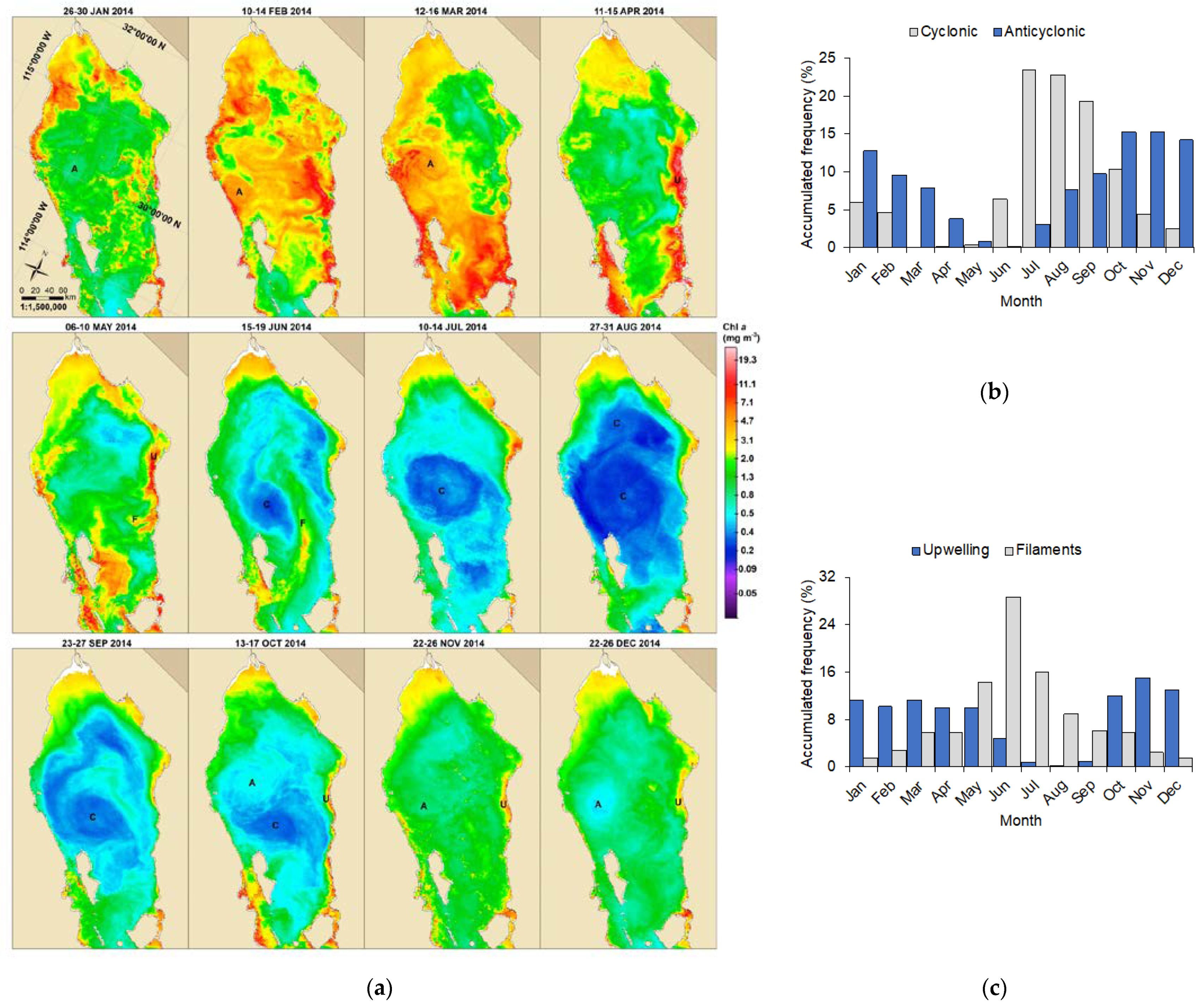
3.1. Annual Analysis (1998–2019) of the Observed Oceanic Mesoscale Events in the Gulf of California

Throughout the gulf, a total of 536 cyclonic eddies, 531 anticyclonic eddies, 758 upwelling events and 603 filaments were identified. The water mass intrusion was identified every year from the gulf´s entrance up to the region south of the Midriff Islands. After the 22-year satellite image analysis, it was observed that the occurrence of eddies differed visually among areas in the gulf. The region north of the Midriff Island showed a noticeable seasonal behavior in the annual frequency of cyclonic and anticyclonic eddies in comparison to the southernmost region of the gulf that presented less variability throughout the year. Applying a Wilcoxon–Mann–Whitney test (p < 0.05) for comparing the annual frequency of eddies showed that the Gulf of California can be divided into three regions: the Northern Gulf of California (NGC) comprises the area north of the Midriff Islands including the Tiburón Basin; the Central Gulf of California (CGC) encompasses the area just south of the Midriff Islands down to the 25°N latitude; while the Southern Gulf of California (SGC) includes the area from the 25°N to the 22°N latitude. From this point on, results will be presented for each one of these regions.

The year 2014 represents a typical year where the different mesoscale events could be identified by means of Chl a satellite images as they best exhibit gradients that eased the identification of the events. Figure 2a shows that during a typical year in the NGC, in fall and winter anticyclonic eddies are more dominant, whereas in summer cyclonic eddies prevail. Just before the formation of the dominant summer eddy, long filaments originate from the Midriff islands and travel to the NGC, they usually present a higher duration than other filaments in the region. The pigment concentration within the anticyclonic eddy increases when vertical mixing and coastal upwelling are more intense and frequent.

In the NGC, a total of 44 cyclonic eddies were identified; only two eddies per year appeared during most of the years of study. In a typical year, the eddy activity took place mostly from June to October, representing 82% of the total eddy frequency. (Figure 2b). The frequency of cyclonic eddies progressively starts earlier in the summer (late June to early June) during the period of this study. The cluster analysis groups the months with similar annual frequency; moreover, July–September was identified as the cluster with the highest frequency, followed by June and October (Figure 3a). For anticyclonic eddies, 99 were identified, which in a typical year showed more activity from October to January, corresponding to 57% of the total frequency, followed by September and February (Figure 2b). The cluster analysis in Figure 3b shows that their frequency can be divided in three periods: October–February are grouped together, as period of the year that presents the highest frequency of anticyclonic eddies, followed by August–September, while March–July showed the lowest frequency.

Coastal upwelling events occurred mostly during October–May (93% of the total frequency), with increased presence during October–December (Figure 2c). During most of winter and spring (January–May) the frequency of these events declined during the period of this study, showing low frequency in 2015–2017. The cluster analysis in Figure 3c shows that the frequency of these events can be divided in three periods, one with high frequency of events (October–December), another period with intermediate frequency (January–May), and a third period with much fewer or an absence of events (June–September). Filaments were identified in all the months; however, during summer (May–July) they represented ~59% of the total frequency, with a peak in June (Figure 2c). Figure 3d shows that June is isolated in the cluster analysis due to its highest frequency during the year, followed by May and July which are grouped together. On the other hand, during the coastal upwelling season of October–December and January–April, a similar frequency of filament events is exhibited, which is the reason why they are in one cluster.

Figure 4a exhibits typical conditions in the CGC; along this region a series of eddies can develop with different rotation. It seems that the amount of Chl a contained by the eddies depends on the season they originate in as the summer eddies show low Chl a concentrations independently of their rotation, while they show relatively higher concentration of pigment during the coastal upwelling period. Filaments can be seen originating from the coastal upwelling mostly from the eastern coast, and sometimes these filaments curl and eventually an eddy may form. The arrival of the water mass intrusion in these regions usually starts in May when a series of eddies with low pigment concentration form; and it exits usually during November, when the coastal upwelling period starts, triggering higher Chl a concentration.

A total of 209 cyclonic eddies were observed in the CGC; as shown in Figure 4b, during a typical year they presented higher frequency during August, followed by July, September and January, with 54% of the total eddy activity. During July–September and January, 2–3 events predominated in frequency, agreeing with the period of highest presence. The cluster analysis in Figure 5a supports these observations, showing July–September in one cluster, representing the months with highest frequency, followed by the second group (January). As for anticyclonic eddies, 203 were identified, showing the highest frequency during September–November, a period that contains 40% of the total frequency (Figure 4b). During the period of this study, a progressive increase from 4 up to 30 days with eddy activity was observed in August. Figure 5b shows that October and November represent a cluster as the months with highest frequency, followed by July–September and the December–February cluster.

A total of 271 coastal upwelling events were identified, showing high frequency during November–April, representing 80% of the total frequency (Figure 4c). In years such as 1999 and 2000, high frequency was also present during May, however, during autumn–winter 2006–2009, low frequencies were observed, as well as during winter–spring of 2014–2016. The cluster analysis in Figure 5c illustrates the annual periodicity of coastal upwelling events, which are more frequent during November–April, and less frequent or absent from June to September. A total of 298 filaments were identified, which in a typical year presented higher frequency during March and April, presenting 2–4 filaments simultaneously; this period contained 43% of the total frequency (Figure 4c). Figure 5d shows the cluster analysis, where March has the highest frequency, followed by a second cluster (February, April and May), corresponding to months with a frequency of coastal upwelling events. The water mass intrusion was identified in all the years of study, exhibiting two annual periods—one with high frequency during May–November, and the other period (December–April) with less frequency or absence of this event (Figure 5e).

Figure 6a shows less typical conditions in the SGC. Along this region, usually a series of eddies developed with different rotation throughout the year. However, the coastal upwelling frequency was lower than normal, present only in April, May and December. Low frequency of filaments was observed due to the low frequency of upwelling events. The water mass intrusion arrived into this region earlier than normal (April) and withdrew in November.

A total of 283 cyclonic eddies were observed in the SGC; the highest frequency was identified during summer months (33% of the total frequency) when three and sometimes four eddies could be observed simultaneously (Figure 6b). As of 2008, these high frequencies progressively increased, starting earlier in May and sometimes starting in mid-April. The cluster analysis in Figure 7a shows that these eddies present two periods, one with relatively high frequency (June–September, January), and a second period (February–May and October–December) showing relatively less frequency. Additionally, 229 anticyclonic eddies were identified, showing high frequency throughout all the year, except during June and July; the highest frequency can be observed during October–April, representing 67% of the total frequency (Figure 6b), where three–four eddies concurred in several years. The cluster analysis in Figure 7b supports that these eddies occurred all-year-round and just sporadically during June and most of July. Coastal upwelling events (203) were identified with higher frequency from November to April of the following year, accounting foe 79% of the total frequency (Figure 6c). During autumn–winter of some years (2002, 2006, 2008, 2009, 2012–2015), these events presented low or null frequency. Filaments (164) were identified, in a typical year showing higher frequency during January–April, accounting for 61% of the total frequency (Figure 6c). As of 2013, a decrease was observed in the annual frequency of these events. Water mass intrusion was identified in all the years of study, showing high frequency from May to November. Some years (1998, 2014–2016) this intrusion could be observed arriving in March. This event shows two periods: one of absence or low frequency (December–April) and another period with high frequency (May–November) (Figure 7e).

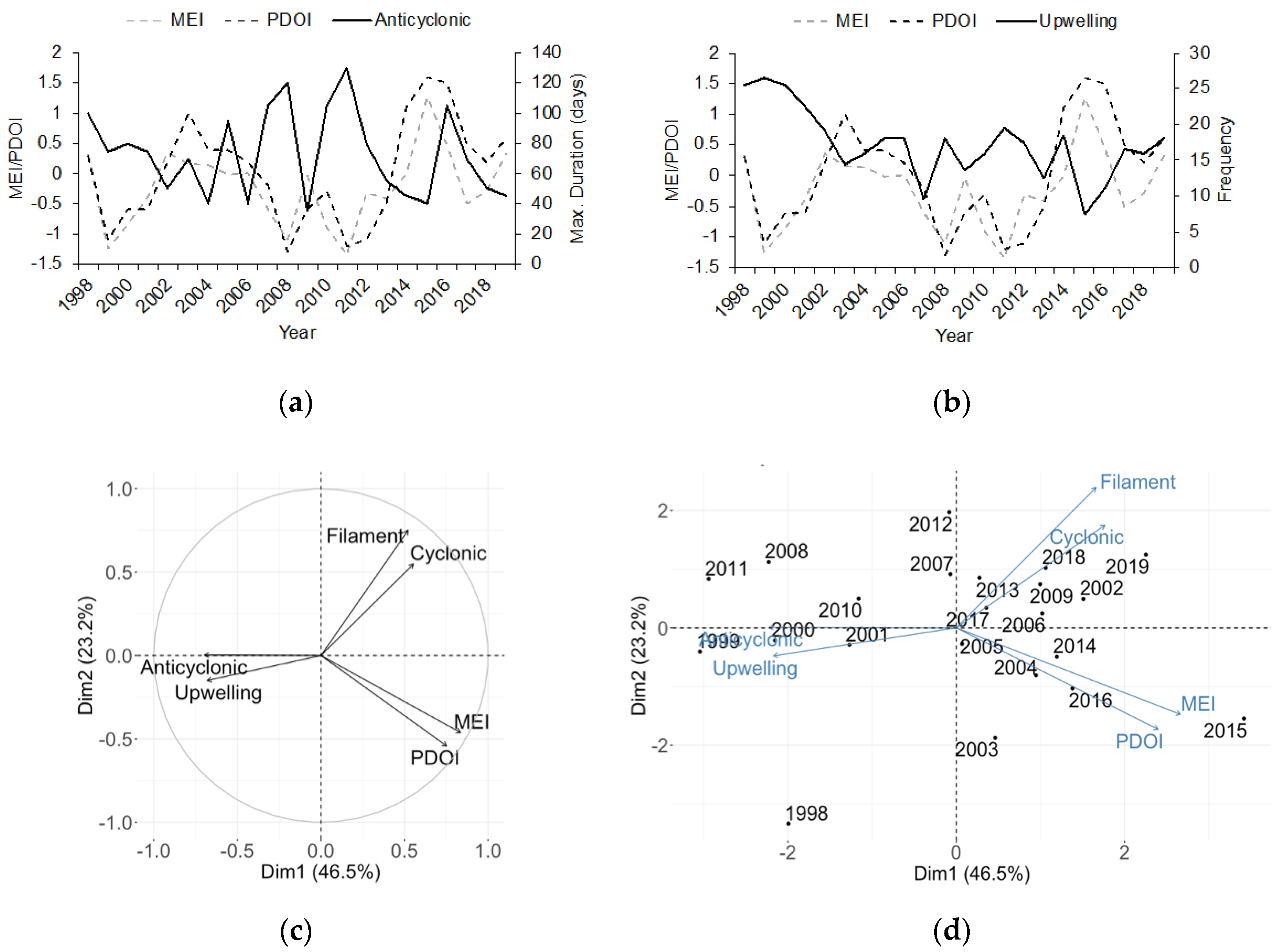
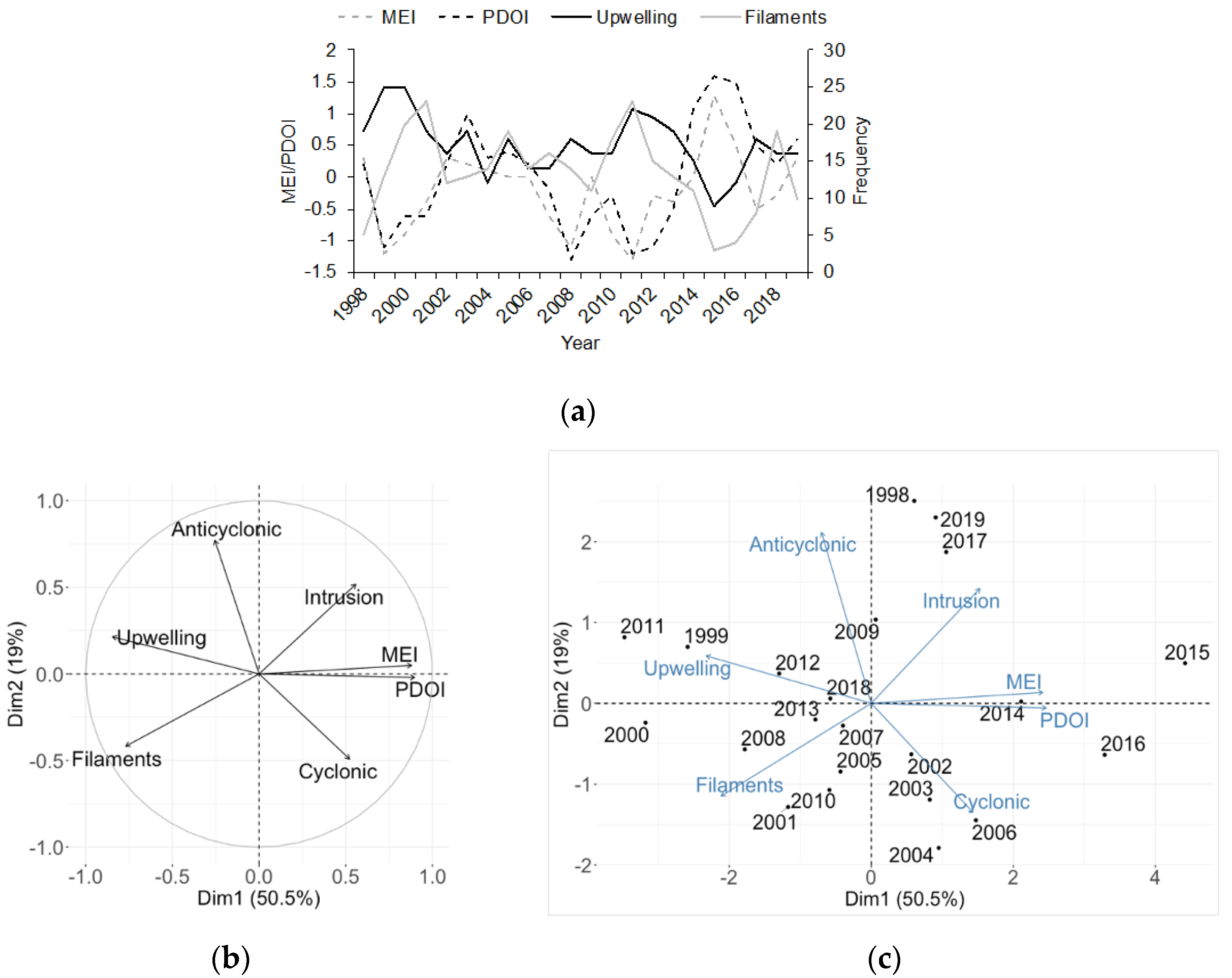
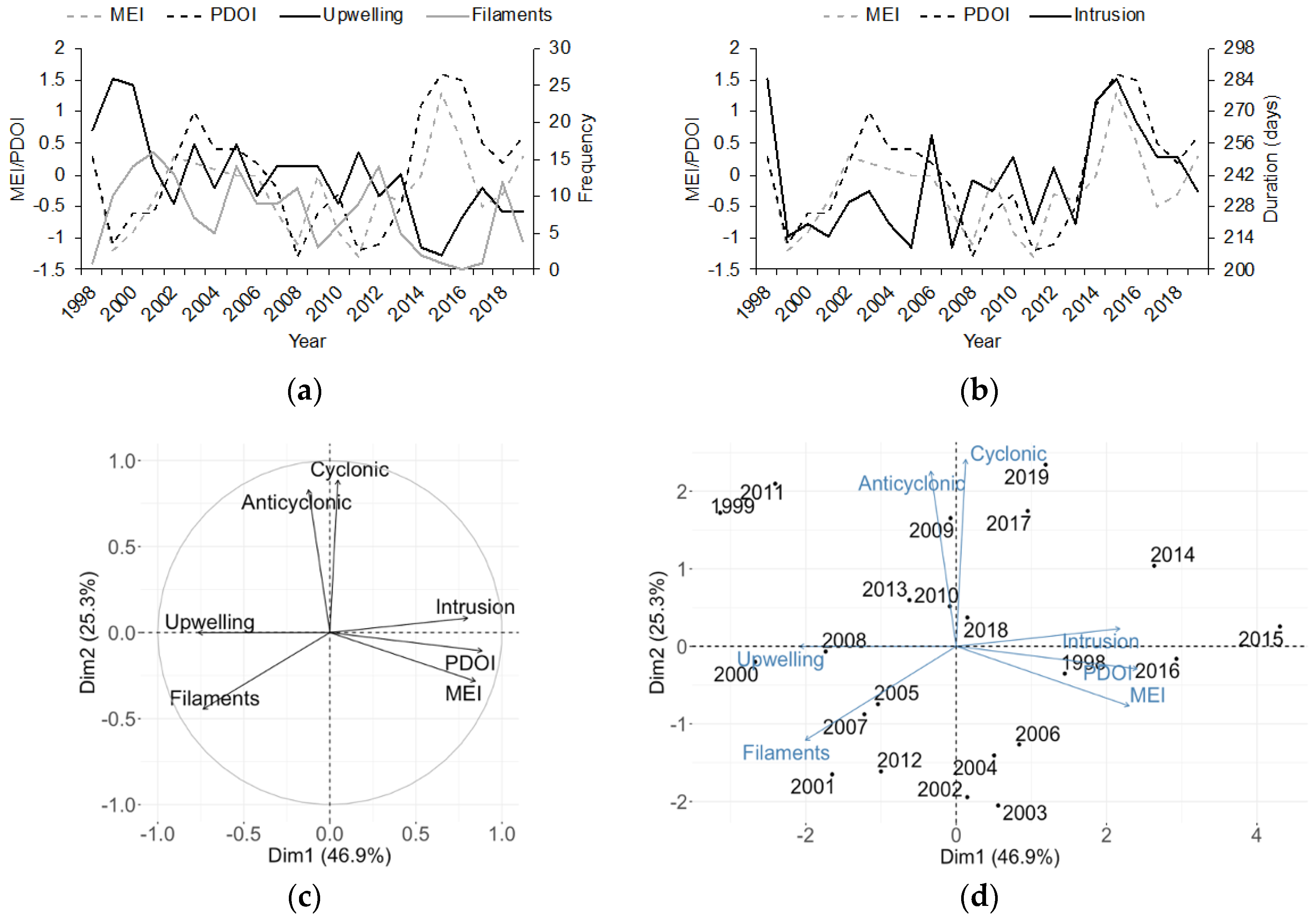
3.2. Interannual Variability of Oceanic Mesoscale Events in the Gulf of California and Climate Indices (MEI and PDOI)

Figure 8a shows chlorophyll a satellite images of the NGC under positive/negative ENSO and PDO conditions. Anticyclonic eddy activity is reduced ~37% under El Niño and positive PDO with respect to La Niña and negative PDO conditions (Figure 8b). Coastal upwelling is reduced ~30% during El Niño and positive PDO with respect to La Niña and negative PDO conditions (Figure 8c).

Figure 9a,d show Chl a and SST satellite images, respectively, of the CGC under positive/negative ENSO and PDO conditions. Coastal upwelling activity is reduced by ~38% during El Niño and positive PDO with respect to La Niña and negative PDO conditions (Figure 9b). Mean annual frequency of filaments is reduced by ~55% during El Niño and positive PDO with respect to La Niña and negative PDO conditions (Figure 9c). The mean annual duration of the water mass intrusion increases ~5% during positive ENSO and PDO with respect to negative conditions (Figure 9e).

Figure 10a,d show Chl a and SST satellite images, respectively, of the SGC under positive/negative ENSO and PDO conditions. Coastal upwelling activity is reduced by ~64% during El Niño and positive PDO with respect to La Niña and negative PDO conditions (Figure 10b). Mean annual frequency of filaments is reduced ~80% during El Niño and positive PDO with respect to La Niña and negative PDO conditions (Figure 10c). The mean annual duration of the water mass intrusion increases ~12% during positive ENSO and PDO with respect to negative conditions (Figure 10e).

In the NGC, the maximum duration of anticyclonic eddies was affected by strong El Niño and positive PDOI of 2014 and 2015, whereas under strong La Niña conditions and negative PDOI (1999–2000, 2007–2008, 2010–2011), the duration of these eddies was enhanced (Figure 11a). In this region, high frequency of coastal upwelling was reported during strong La Niña and negative PDOI of 1999–2001, 2008 and 2011. The opposite was observed during strong El Niño and positive PDOI such as in 2015–2016 (Figure 11b).

The PCA estimated that ~70% of the variance was explained by the first two principal components—Dim 1 (PC1) with an eigenvalue of 2.79 explaining 46.5%, Dim2 (PC2) with an eigenvalue of 1.39 explaining 23.2%. MEI, PDOI, anticyclonic eddies and coastal upwelling were variables that significantly contributed to the PC1, whereas filaments, cyclonic eddies and PDOI were variables with significant contribution to the PC2 (Figure 11c). The years that significantly contributed to PC1 exhibited concurrently positive and negative MEI and PDOI values. The years that significantly contributed to PC2 exhibited warm or cold periods in the El Niño 3.4 region, as well as synchronicity in the positive and negative values of both climate indices (Figure 11d).

Table 1. Significantly associated variables within principal component 1 and 2 in the Northern Gulf of California.

PC1
Variable	Correlation	p-Value
MEI	0.84	1.35 × 10−6
PDOI	0.75	5.47 × 10−5
Cyclonic	0.55	7.53 × 10−3
Filaments	0.52	1.30 × 10−2
Coastal upwelling	−0.68	4.89 × 10−4
Anticyclonic	−0.70	3.09 × 10−4
PC2
Variable	Correlation	p-Value
Filaments	0.75	5.95 × 10−5
Cyclonic	0.55	8.32 × 10−3
MEI	−0.46	3.04 × 10−2
PDOI	−0.54	9.09 × 10−3

displays the most significantly associated variables within PC1 and PC2; it shows that in PC1 the MEI and PDOI are directly correlated with cyclonic eddies and filaments but inversely correlated with coastal upwelling and anticyclonic eddies. In the PC2, filaments and cyclonic eddies are inversely correlated with the MEI and PDOI.

In the CGC, the frequency of upwelling events and filaments decreased in the 2015–2016 El Niño and under positive PDOI, while during strong la Niña and under negative PDOI of 1999–2000 and 2011–2012, their frequency was higher (Figure 12a). The PCA assessed that ~70% of the variance was explained by the first two PC; PC1 with eigenvalue of 3.54 explained 51%, while PC2 with eigenvalue of 1.33 explained 19%. The variables that significantly contributed to PC1 were PDOI, MEI, coastal upwelling and filaments; whereas, anticyclonic and cyclonic eddies and water mass intrusion significantly contributed to PC2 (Figure 12b). The years that had a significant contribution to PC1 exhibited warm and cold periods as well as synchronicity of high positive and negative anomalies of MEI and PDOI. The years that significantly contributed to PC2 exhibited warm periods and synchronicity in positive and negative anomalies of both indices; whereas, 2004, 2006 and 2001 presented short periods of warm or cold periods but no synchronicity of PDOI and MEI anomalies (Figure 12c).

Table 2. Significantly associated variables within principal component 1 and 2 in the Central Gulf of California.

PC1
Variable	Correlation	p-Value
PDOI	0.90	1.53 × 10−8
MEI	0.88	6.69 × 10−8
Intrusion	0.56	6.97 × 10−3
Cyclonic	0.52	1.26 × 10−2
Filaments	−0.77	2.78 × 10−5
Coastal upwelling	−0.85	6.95 × 10−7
PC2
Variable	Correlation	p-Value
Anticyclonic	0.77	2.68 × 10−5
Intrusion	0.52	1.37 × 10−3
Cyclonic	−0.49	2.01 × 10−2

presents the most significantly associated variables within PC1 and PC2; it shows that in PC1, the MEI and PDOI are directly correlated with cyclonic eddies and water mass intrusion but inversely correlated with coastal upwelling and filaments. In the PC2, anticyclonic eddies and water mass intrusion are directly correlated, and both of them are inversely correlated with cyclonic eddies.

In the SGC, the frequency of upwelling events and filaments decreased in the 2015–2016 El Niño and positive PDOI, while during strong La Niña and negative PDOI of 1999–2000 and 2011–2012, their frequency was higher (Figure 13a). The duration of the water mass intrusion was enhanced during the strong El Niño and positive PDOI of 1997–1998, 2015–2016. During strong La Niña and negative PDOI (1999–2000, 2007–2008, 2011), its duration was reduced (Figure 13b).

The PCA assessed that ~72% of the variance was explained by the first two PC; with PC1 with eigenvalue of 3.28 explaining 47%, while PC2 with eigenvalue of 1.77 explained 25%. The PDOI, MEI, water mass intrusion, coastal upwelling and filaments were the variables that significantly contributed to PC1, while cyclonic and anticyclonic eddies were the ones that significantly contributed to PC2 (Figure 13c). The years that significantly contributed to PC1 exhibited either warm or cold events and synchronicity of positive and negative anomalies of the PDOI and MEI, with the exception of 2014 which presented high positive anomalies of PDOI only (Figure 13d). Most of the years that significantly contributed to PC2 exhibited cold or warm periods and synchronicity of positive and negative anomalies of the PDOI and MEI (Figure 13d).

Table 3. Significantly associated variables within principal component 1 and 2 in the Southern Gulf of California.

PC1
Variable	Correlation	p-Value
PDOI	0.88	4.62 × 10−8
MEI	0.85	7.31 × 10−7
Intrusion	0.80	7.85 × 10−6
Filaments	−0.74	9.13 × 10−5
Coastal upwelling	−0.76	3.39 × 10−5
PC2
Variable	Correlation	p-Value
Cyclonic	0.89	4.03 × 10−8
Anticyclonic	0.83	1.71 × 10−6
Filaments	−0.44	3.80 × 10−2

presents the most significantly associated variables within PC1 and PC2; it shows that in PC1, the PDOI and MEI are directly correlated with the water mass intrusion but inversely correlated with coastal upwelling and filaments. In the PC2, cyclonic and anticyclonic eddies are directly correlated, and both of them are inversely correlated with filaments.

4. Discussion

In the NGC, cyclonic eddies were more frequent and with greater lifespan during summer (June–October), whereas anticyclonic eddies were more frequent and with higher lifespan during autumn–winter (October–January). Marinone [56] identified that the semiannual behavior of the Langranian circulation, which is representative of the surface ocean currents, is due to hydrographic forcing, with the Pacific Ocean being the most important. The wind and heat fluxes are responsible for the semiannual variability, while the Pacific Ocean is responsible for the annual variability of the surface currents which are responsible for the formation of these eddies in the NGC [34]. Additionally, in our study, relatively smaller and shorter-lifespan anticyclonic and cyclonic eddies were observed during the summer cyclonic circulation and the winter anticyclonic circulation, respectively. These observations were not detected by numerical modelling or hydrographic data, however, Gutiérrez et al. [34] using a Langranian circulation model observed a small cyclonic eddy during winter. Furthermore, López-Calderón et al. [57], using Chl a satellite images and wind data, observed this behavior of the eddies in the NGC; they identified the importance of the wind component across the GC (u’) in the formation of these less persistent and smaller eddies.

Although the NGC is relatively shallow in comparison to the central and southern regions, coastal upwelling has been reported in its eastern coast by Lluch-Cota [58], showing a seasonal pattern and being more frequent during the period of northwestern winds (October–May), as documented in this study. Filaments were observed during this period of high upwelling frequency generated by wind forcing; these structures transported cold nutrient-rich water offshore. Furthermore, contrary to what happens in the central and southern regions, the highest frequency of filaments was observed early in the summer when long filaments originated from the Midriff Islands region, transporting cold and high Chl a water to the NGC. There is communication throughout the year between the NGC and the rest of the gulf through the channels between Angel de La Guarda and Tiburon islands (Tiburon Basin), only inhibited when anticyclonic circulation is present in the NGC and the rest of the gulf (May and October–November) [34]. Badan-Dangon et al. [59] and Paden et al. [60] using SST satellite images observed these plumes (filaments) that originated from the Midriff islands and transported cold surface water to the NGC. The summer filaments from the Midriff islands found in this study connected with the NGC through the Tiburon Basin. During summer, cyclonic circulation predominates in the entire gulf, enhancing the formation of these structures which could have important implications in the transport of planktonic organisms between these regions.

The Pacific Ocean is the main forcing in the GC, it occurs in the annual frequency via an internal baroclinic Kelvin wave that enters in the eastern GC [61]. Gutiérrez et al. [34] identified one period of cyclonic circulation from July to August in the central and southern regions. The wind also plays an important role as forcing agent for ocean surface circulation in these regions, in general being southward during winter and northward during summer [35]. In this study the higher occurrence and frequency of cyclonic eddies were observed during summer (July to September) in the CGC, which responds to both the Pacific Ocean and the summer wind regime, where the interaction of both may enhance the duration of these eddies, as could be seen in this study where the maximum duration of cyclonic eddies were reported during summer months. Furthermore, local wind and coastal trapped waves can enhance or weaken the poleward eastern boundary current that enters the GC which interacts with the capes and ridges along the CGC and SGC for the generation of eddies [15]. As seen from the Chl a satellite images, overall, in the GC the pigment concentration of eddies depends more on the season in which they occur and on the coast where they originate. This enables them, depending on their rotation, to concentrate or disperse eutrophic or oligotrophic water from one area to another and affect plankton distribution with effects on coastal an pelagic fauna [14]; these same observations were made by López-Calderón et al. [57] for the NGC analyzing Chl a satellite images.

The central and southern regions have two periods of anticyclonic circulation from October to November and in May; furthermore, from January to March, wind induces currents to flow to the mouth of the gulf [34,62]. The equatorward flow of these two forcing agents and their combined interaction along the coasts of the central and southern regions would be responsible for the high occurrence/frequency of anticyclonic eddies during fall and winter in the CGC; likewise, the maximum duration of these eddies was reported during fall–winter, when both forcing agents enhance the eddies duration. However, in the SGC, the occurrence/frequency of eddies shows less seasonality, being frequent almost throughout the entire year. This region is in direct communication with the Pacific Ocean and is part of a convergence zone where waters from the California Current, equatorial surface waters carried by the Mexican Coastal Current and the Gulf of California waters with high salinity meet, generating mesoscale meanders and eddies [37,63]. Considering the confluence of these water masses and the proposed hypothesis by Zamudio et al. [15] that the interaction of the MCC with the coastline when it intensifies while entering the SGC generates a series of eddies in this region, it is then expected that during most of the year, there will be the presence of cyclonic and anticyclonic eddies depending on the surface currents and wind direction.

The periods for coastal upwelling event recorded in this study for the CGC and SGC are similar to that reported by Lluch-Cota [58] using a wind-derived index and by García Morales et al. [14] using Chl a satellite images. The use of SST satellite images to detect alongshore surface temperature gradients as a proxy for identifying upwelling events has been used in other regions [44,45]. Although the wind was not included for the identification of this event, the use of SST gradients could be of utility to observe the physical (SST) and biological response (Chl a concentration) to this wind forcing. It can give an idea of how stratified the water column is and that despite there being wind forcing, if the thermocline is deeper than normal, the upwelling mechanism will be hard to achieve. This could happen with the intensification of the MCC through coastal Kelvin waves that could deepen the thermocline in the eastern coast of the GC [13,64].

Filaments originating from coastal upwelling had a similar behavior in both the central and southern region. They were more frequent in the CGC than in the SGC, probably because the former has a more irregular coastline with capes and ridges, and as wind forcing during winter and spring generate equatorward currents, they may interact with these coastal features to enhance the formation of these structures [65,66]. These filaments with cold and pigment-rich water are important mechanisms for offshore transport of eggs and larvae of ecological and economic important marine species with consequences for their survival and recruitment [14].

The seasonal movement of the Inter-Tropical Convergence Zone causes latitudinal displacements of the equatorial current system, determining how far north the Costa Rica Coastal Current will carry Tropical Surface Water [62]. Additionally, the Mexican Coastal Current (MCC) reaches the GC during spring and fall, showing a seasonal behavior, the intensity of which greatly depends on equatorial Kelvin waves [67,68]. This explains the seasonal intrusion of warm (25 °C) and oligotrophic (~0.3 mg m⁻³ Chl a) water mass to the SGC and CGC found in this study, usually from April to November, some years arriving earlier and/or retreating later due to the poleward enhancement from internal Kelvin waves. This agrees with the observations made by García-Morales et al. [14] using monthly satellite images for the central coast of Sonora, mentioning that the fronts created by the intrusion are important mechanisms of plankton retention and species distribution.

The PCA analysis allowed to identify hidden patterns in the dataset and identified correlated variables. In the NGC, it was observed that the interannual variability of cyclonic and anticyclonic eddies’ maximum duration, coastal upwelling frequency, and filaments’ average duration was influenced by very strong El Niño and La Niña events represented by the MEI values, influenced also by positive and negative PDOI values. Lavín and Marinone [62] identified that the ENSO is accountable for the strongest interannual anomalies in the GC, and during El Niño events, internal coastal trapped waves can deepen 50 to 100 m the surface mixed layer and thermocline. This would explain the negative effects of El Niño events on the interannual frequency of coastal upwelling, where the thermocline is deeper than average so that subsurface, cold, nutrient-rich water is not sufficiently upwelled to the surface. This effect should also apply to the frequency of coastal upwelling and subsequently of filaments in the central and southern gulf regions, as was observed in the results of this study.

The circulation in the NGC is more susceptible to short wind events and to interannual events like ENSO, particularly during the anticyclonic phase when the barotropic component is important [39,69]. The results in this study, shown in the PCA analysis, identified the maximum duration of anticyclonic eddies as being negatively affected by strong El Niño conditions and positive PDOI values, probably because of weakening of northwestern winds and due to the strengthening of internal Kelvin waves affecting the barotropic condition.

Gómez-Valdivia et al. [68] observed that under El Niño conditions, in addition to the variability of internal Kelvin waves, there is an increase in the velocity of alongshore currents, enhancing the effects of the MCC in the GC. These mixed effects during positive ENSO periods, and during positive PDOI values, should be responsible for the increase of the duration of summer filaments and cyclonic eddies duration, as shown in the PCA analysis.

The interannual variability of mesoscale events in the CGC shows that water mass intrusion and cyclonic eddies frequency may be enhanced with strong El Niño conditions together with positive PDOI values; furthermore, the increase in duration of the water intrusion shows an increase in the frequency of anticyclonic eddies. The enhancement of the MCC current due to stronger coastal trapped waves during positive ENSO periods should indicate a stronger interaction of these poleward currents with the coastline, increasing the formation of cyclonic and anticyclonic eddies in this region [14,15].

In the SGC, no effect of interannual variability (ENSO or PDOI) was observed over the frequency of eddies. In this region, there is interaction between the California current water, the tropical surface water and the Gulf of California water, thus presenting transitional thermohaline characteristics [62,63]. Additionally, the region presents very high lateral variability in the geostrophic velocity, exhibiting numerous mesoscale eddies [62,70]. It seems that except under strong El Niño/La Niña conditions, the seasonal variability is the most relevant with regards to the large-scale interaction between the southern branch of the California current and the Mexican Coastal Current [67,71]. Furthermore, from this region and northward, the influence of ENSO is more restricted to the eastern coastal area [67], as could be observed in our results, higher presence of water intrusion associated with positive MEI and PDOI values. This is probably why the effects of ENSO and/or PDOI are not fully observed in this region, since many of the eddies identified were relatively far from the coast, as seen from the satellite images, and possibly originated from barotropic instabilities due to the interaction of the water masses [63].

The results show that the occurrence and frequency of these mesoscale events vary annually in the different regions of the GC, as each one of these areas exhibits distinct depth, bathymetry, coastline, local wind and surface current conditions. Additionally, constantly monitoring these oceanic events and their variability due to climate events that take place on a wider spatial and temporal scale, will help in the understanding of how the different regions of this large marine ecosystem respond to these variations in the long term. These mesoscale events are important for the concentration, transport and dispersal of nutrients, pigments, planktonic organisms, including eggs and larvae, consequently affecting the distribution and abundance of numerous marine species of ecological and economic importance [14,72].

5. Conclusions

The use of SST and Chl a satellite images with a 5-day temporal resolution allowed to better identify and quantify each mesoscale event and its duration. These permitted to observe a seasonal behavior of these events in the NGC followed by the CGC. In the SGC, due to the interaction of various water masses with distinct characteristics, less evident seasonality was exhibited in the frequency of eddies.

The use of satellite images to detect coastal SST gradients can be a good proxy for identifying coastal upwelling events. Further research can focus on integrating wind forcing with SST gradients to better understand the variability of this event and its consequent effects on the coastal and adjacent regions.

The interannual variability of mesoscale events significantly responded to strong El Niño and La Niña events, as well as to positive and negative phases of the PDOI. This shows that the signal and effects that these large-scale climate events can have in the GC depend on their intensity and the interaction among them. This work highlights the importance of using satellite imagery to study in the long term and at different spatial scales marine ecosystem dynamics and variability.

References

1. Oschlies, A.; Garçon, V. Eddy-induced enhancement of primary production in a model of the North Atlantic. Nature 1998, 394, 266–269. [Google Scholar] [CrossRef]
2. López-Calderón, J.; Manzo-Monroy, H.; Santamaría-del-Ángel, E.; Castro, R.; González-Silvera, A.; Millán-Núñez, R. Mesoscale variability of the Mexican Tropical Pacific using TOPEX and SeaWiFS data. Cienc. Mar. 2006, 32, 539–549. [Google Scholar] [CrossRef]
3. Fu, L.-L.; Chelton, D.B.; Le Traon, P.-Y.; Morrow, R. Eddy Dynamics From Satellite Altimetry. Oceanography 2010, 23, 14–25. [Google Scholar] [CrossRef] [Green Version]
4. Alpers, W.; Brandt, P.; Lazar, A.; Dagorne, D.; Sow, B.; Faye, S.; Hansen, M.W.; Rubino, A.; Poulain, P.-M.; Brehmer, P. A small-scale oceanic eddy off the coast of West Africa studied by multi-sensor satellite and surface drifter data. Remote Sens. Environ. 2013, 129, 132–143. [Google Scholar] [CrossRef]
5. Cruz Gómez, R.C.; Monreal Gómez, M.A.; Nikolaevich Bulgakov, S. Efecto de los vórtices en sistemas acuáticos y su relación con la química, biología y geología. Interciencia 2008, 33, 741–746. [Google Scholar]
6. Kahru, M.; Fiedler, P.C.; Gille, S.T.; Manzano, M.; Mitchell, B.G. Sea level anomalies control phytoplankton biomass in the Costa Rica Dome area. Geophys. Res. Lett. 2007, 34, 1–5. [Google Scholar] [CrossRef] [Green Version]
7. Kahru, M.; Mitchell, B.G.; Gille, S.T.; Hewes, C.D.; Holm-Hansen, O. Eddies enhance biological production in the Weddell-Scotia Confluence of the Southern Ocean. Geophys. Res. Lett. 2007, 34, 1–6. [Google Scholar] [CrossRef] [Green Version]
8. Dufois, F.; Hardman-Mountford, N.J.; Greenwood, J.; Richardson, A.J.; Feng, M.; Matear, R.J. Anticyclonic eddies are more productive than cyclonic eddies in subtropical gyres because of winter mixing. Sci. Adv. 2016, 2, e1600282. [Google Scholar] [CrossRef] [PubMed] [Green Version]
9. Gaube, P.; Chelton, D.B.; Samelson, R.M.; Schlax, M.G.; O’Neill, L.W. Satellite Observations of Mesoscale Eddy-Induced Ekman Pumping. J. Phys. Oceanogr. 2015, 45, 104–132. [Google Scholar] [CrossRef]
10. Wang, Y.; Zhang, H.-R.; Chai, F.; Yuan, Y. Impact of mesoscale eddies on chlorophyll variability off the coast of Chile. PLoS ONE 2018, 13, e0203598. [Google Scholar] [CrossRef]
11. Chaigneau, A.; Eldin, G.; Dewitte, B. Eddy activity in the four major upwelling systems from satellite altimetry (1992–2007). Prog. Oceanogr. 2009, 83, 117–123. [Google Scholar] [CrossRef]
12. Nan, F.; Xue, H.; Xiu, P.; Chai, F.; Shi, M.; Guo, P. Oceanic eddy formation and propagation southwest of Taiwan. J. Geophys. Res. Ocean. 2011, 116, 1–15. [Google Scholar] [CrossRef] [Green Version]
13. Lluch-Cota, S.E.; Aragón-Noriega, E.A.; Arreguín-Sánchez, F.; Aurioles-Gamboa, D.; Jesús Bautista-Romero, J.; Brusca, R.C.; Cervantes-Duarte, R.; Cortés-Altamirano, R.; Del-Monte-Luna, P.; Esquivel-Herrera, A.; et al. The Gulf of California: Review of ecosystem status and sustainability challenges. Prog. Oceanogr. 2007, 73, 1–26. [Google Scholar] [CrossRef]
14. García-Morales, R.; López-Martínez, J.; Valdez-Holguin, J.E.; Herrera-Cervantes, H.; Espinosa-Chaurand, L.D. Environmental Variability and Oceanographic Dynamics of the Central and Southern Coastal Zone of Sonora in the Gulf of California. Remote Sens. 2017, 9, 925. [Google Scholar] [CrossRef] [Green Version]
15. Zamudio, L.; Hogan, P.; Metzger, E.J. Summer generation of the Southern Gulf of California eddy train. J. Geophys. Res. Ocean. 2008, 113, 1–21. [Google Scholar] [CrossRef] [Green Version]
16. Robles-Tamayo, C.M.; Valdez-Holguín, J.E.; García-Morales, R.; Figueroa-Preciado, G.; Herrera-Cervantes, H.; López-Martínez, J.; Enríquez-Ocaña, L.F. Sea Surface Temperature (SST) Variability of the Eastern Coastal Zone of the Gulf of California. Remote Sens. 2018, 10, 1434. [Google Scholar] [CrossRef] [Green Version]
17. Brusca, R.; Hendrickx, M.E. Invertebrate biodiversity and conservation in the Gulf of California. In The Gulf of California Biodiversity and Conservation; Brusca, R., Ed.; The University of Arizona Press: Tucson, AZ, USA, 2010; pp. 72–95. [Google Scholar]
18. Páez-Osuna, F.; Sanchez-Cabeza, J.A.; Ruiz-Fernández, A.C.; Alonso-Rodríguez, R.; Piñón-Gimate, A.; Cardoso-Mohedano, J.G.; Flores-Verdugo, F.J.; Carballo, J.L.; Cisneros-Mata, M.A.; Álvarez-Borrego, S. Environmental status of the Gulf of California: A review of responses to climate change and climate variability. Earth-Sci. Rev. 2016, 162, 253–268. [Google Scholar] [CrossRef]
19. Arreguín-Sánchez, F.; Del Monte-Luna, P.; Zetina-Rejón, M.J.; Albáñez-Lucero, M.O. The Gulf of California Large Marine Ecosystem: Fisheries and other natural resources. Environ. Dev. 2017, 22, 71–77. [Google Scholar] [CrossRef]
20. Melo, F.J.F.R.; Suárez-Castillo, A.; Amador-Castro, I.G.; Gastélum-Nava, E.; Espinosa-Romero, M.J.; Torre, J. Bases para el ordenamiento de la pesca artesanal con la participación del sector productivo en la Región de las Grandes Islas, Golfo de California. Cienc. Pesq. 2018, 26, 81–100. [Google Scholar]
21. Lanz, E.; López-Martínez, J.; Nevárez-Martínez, M.; Dworak, J.A. Small pelagic fish catches in the Gulf of California associated with sea surface temperature and chlorophyll. Calif. Coop. Ocean. Fish. Investig. Rep. 2009, 50, 134–146. [Google Scholar]
22. Early, J.J.; Samelson, R.M.; Chelton, D.B. The Evolution and Propagation of Quasigeostrophic Ocean Eddies*. J. Phys. Oceanogr. 2011, 41, 1535–1555. [Google Scholar] [CrossRef]
23. Nurser, A.J.G.; Zhang, J.W. Eddy-induced mixed layer shallowing and mixed layer/thermocline exchange. J. Geophys. Res. Ocean. 2000, 105, 21851–21868. [Google Scholar] [CrossRef]
24. Contreras-Catala, F.; Sánchez-Velasco, L.; Lavín, M.F.; Godínez, V.M. Three-dimensional distribution of larval fish assemblages in an anticyclonic eddy in a semi-enclosed sea (Gulf of California). J. Plankton Res. 2012, 34, 548–562. [Google Scholar] [CrossRef] [Green Version]
25. Apango-Figueroa, E.; Sánchez-Velasco, L.; Lavín, M.F.; Godínez, V.M.; Barton, E.D. Larval fish habitats in a mesoscale dipole eddy in the gulf of California. Deep. Sea Res. Part I Oceanogr. Res. Pap. 2015, 103, 1–12. [Google Scholar] [CrossRef]
26. Castelao, R.M.; Mavor, T.P.; Barth, J.A.; Breaker, L.C. Sea surface temperature fronts in the California Current System from geostationary satellite observations. J. Geophys. Res. Ocean. 2006, 111. [Google Scholar] [CrossRef] [Green Version]
27. Kahru, M.; Di Lorenzo, E.; Manzano-Sarabia, M.; Mitchell, B.G. Spatial and temporal statistics of sea surface temperature and chlorophyll fronts in the California Current. J. Plankton Res. 2012, 34, 749–760. [Google Scholar] [CrossRef] [Green Version]
28. Castelao, R.M.; Wang, Y. Wind-driven variability in sea surface temperature front distribution in the California Current System. J. Geophys. Res. Ocean. 2014, 119, 1861–1875. [Google Scholar] [CrossRef]
29. Wang, Y.; Liu, J.; Liu, H.; Lin, P.; Yuan, Y.; Chai, F. Seasonal and Interannual Variability in the Sea Surface Temperature Front in the Eastern Pacific Ocean. J. Geophys. Res. Ocean. 2021, 126, 1–17. [Google Scholar] [CrossRef]
30. McGillicuddy, D.J. Mechanisms of Physical-Biological-Biogeochemical Interaction at the Oceanic Mesoscale. Annu. Rev. Mar. Sci. 2016, 8, 125–159. [Google Scholar] [CrossRef] [PubMed] [Green Version]
31. Lluch-Cota, S.E.; Arias-Aréchiga, J.P. Sobre la importancia de considerar la existencia de centros de actividad biológica para la regionalización del océano: El caso del Golfo de California. In Centros de Actividad Biológica del Pacífico Mexicano; Lluch-Belda, D., Elourduy-Garay, J.F., Lluch-Cota, S.E., Pnce-Díaz, G., Eds.; Centro de Investigaciones Biológicas del Noroeste, SC: La Paz, Mexico, 2000; ISBN 970-18-6285-6. [Google Scholar]
32. Lluch-Cota, S.E.; Parés-Sierra, A.; Magaña-Rueda, V.O.; Arreguín-Sánchez, F.; Bazzino, G.; Herrera-Cervantes, H.; Lluch-Belda, D. Changing climate in the Gulf of California. Prog. Oceanogr. 2010, 87, 114–126. [Google Scholar] [CrossRef]
33. Beier, E. A Numerical Investigation of the Annual Variability in the Gulf of California. J. Phys. Oceanogr. 1997, 27, 615–632. [Google Scholar] [CrossRef]
34. Gutiérrez, O.Q.; Marinone, S.G.; Parés-Sierra, A. Lagrangian surface circulation in the Gulf of California from a 3D numerical model. Deep. Sea Res. Part II Top. Stud. Oceanogr. 2004, 51, 659–672. [Google Scholar] [CrossRef] [Green Version]
35. Jiménez, A.; Marinone, S.G.; Parés-Sierra, A. Efecto de la variabilidad espacial y temporal del viento sobre la circulación en el Golfo de California. Ciencias Mar. 2005, 31, 357–368. [Google Scholar] [CrossRef] [Green Version]
36. Figueroa, J.M.; Lavin, M.F.; Marinone, S.G. A Description of Geotrophic Gyres in the Southern Gulf of California. In Nonlinear Processes in Geophysical Fluid Dynamics; Velasco Fuentes, O.U., Ed.; Kluwer Academic Publishers: Dordrecht, The Netherlands, 2003; pp. 237–255. [Google Scholar]
37. Lavín, M.F.; Castro, R.; Beier, E.; Godínez, V.M.; Amador, A.; Guest, P. SST, thermohaline structure, and circulation in the southern Gulf of California in June 2004 during the North American Monsoon Experiment. J. Geophys. Res. Ocean. 2009, 114. [Google Scholar] [CrossRef]
38. Hofmann, E.E.; Powell, T.M. Environmental Variability Effects on Marine Fisheries: Four Case Histories. Ecol. Appl. 1998, 8, S23–S32. [Google Scholar] [CrossRef] [Green Version]
39. Carrillo, L.; Lavín, M.F.; Palacios-Hernández, E. Seasonal Evolution of the Geostrophic Circulation in the Northern Gulf of California. Estuar. Coast. Shelf Sci. 2002, 54, 157–173. [Google Scholar] [CrossRef]
40. Castro, R.; Lavín, M.F.; Beier, E.; Amador, A. Structure of mesoscale eddies in the southern Gulf of California during cruise NAME-2 (August 2004). In Proceedings of the AGU Spring Meeting, Boulder, CO, USA, May 2007. [Google Scholar]
41. Pegau, W.S.; Boss, E.; Martínez, A. Ocean color observations of eddies during the summer in the Gulf of California. Geophys. Res. Lett. 2002, 29, 6-1–6-3. [Google Scholar] [CrossRef] [Green Version]
42. Cayula, J.-F.; Cornillon, P. Edge Detection Algorithm for SST Images. J. Atmos. Ocean. Technol. 1992, 9, 67–80. [Google Scholar] [CrossRef]
43. Diehl, S.F.; Budd, J.W.; Ullman, D.; Cayula, J.-F. Geographic Window Sizes Applied to Remote Sensing Sea Surface Temperature Front Detection. J. Atmos. Ocean. Technol. 2002, 19, 1105–1113. [Google Scholar] [CrossRef]
44. García-Reyes, M.; Largier, J.L.; Sydeman, W.J. Synoptic-scale upwelling indices and predictions of phyto- and zooplankton populations. Prog. Oceanogr. 2014, 120, 177–188. [Google Scholar] [CrossRef]
45. Dabuleviciene, T.; Kozlov, I.E.; Vaiciute, D.; Dailidiene, I. Remote Sensing of Coastal Upwelling in the South-Eastern Baltic Sea: Statistical Properties and Implications for the Coastal Environment. Remote Sens. 2018, 10, 1752. [Google Scholar] [CrossRef] [Green Version]
46. Strub, P.T.; Kosro, P.M.; Huyer, A. The nature of the cold filaments in the California Current system. J. Geophys. Res. Ocean. 1991, 96, 14743–14768. [Google Scholar] [CrossRef]
47. Artal, O.; Sepúlveda, H.H.; Mery, D.; Pieringer, C. Detecting and characterizing upwelling filaments in a numerical ocean model. Comput. Geosci. 2019, 122, 25–34. [Google Scholar] [CrossRef]
48. Jones, B.H.; Mooers, C.N.K.; Rienecker, M.M.; Stanton, T.; Washburn, L. Chemical and biological structure and transport of a cool filament associated with a jet-eddy system off northern California in July 1986 (OPTOMA21). J. Geophys. Res. Ocean. 1991, 96, 22207–22225. [Google Scholar] [CrossRef]
49. Martínez Flores, G.; Nava Sánchez, E.H.; Zaitzev, O. Teledetección de plumas de material suspendido influenciadas por escorrentía en el sur del golfo de california. Cicimar Oceánides 2011, 26, 1–18. [Google Scholar] [CrossRef]
50. Fiedler, P.C.; Talley, L.D. Hydrography of the eastern tropical Pacific: A review. Prog. Oceanogr. 2006, 69, 143–180. [Google Scholar] [CrossRef]
51. Portela, E.; Beier, E.; Barton, E.D.; Castro, R.; Godínez, V.; Palacios-Hernández, E.; Fiedler, P.C.; Sánchez-Velasco, L.; Trasviña, A. Water Masses and Circulation in the Tropical Pacific off Central Mexico and Surrounding Areas. J. Phys. Oceanogr. 2016, 46, 3069–3081. [Google Scholar] [CrossRef] [Green Version]
52. Bodenhofer, U.; Kothmeier, A.; Hochreiter, S. APCluster: An R package for affinity propagation clustering. Bioinformatics 2011, 27, 2463–2464. [Google Scholar] [CrossRef]
53. Abdi, H.; Williams, L.J. Principal component analysis. Wiley Interdiscip. Rev. Comput. Stat. 2010, 2, 433–459. [Google Scholar] [CrossRef]
54. Kassambara, A.; Mundt, F. Factoextra: Extract and Visualize the Results of Multivariate Data Analyses. R Package Version 1.0.7. Available online: https://cran.r-project.org/package=factoextra (accessed on 10 January 2021).
55. Lê, S.; Josse, J.; Husson, F. FactoMineR: AnRPackage for Multivariate Analysis. J. Stat. Softw. 2008, 25, 1–18. [Google Scholar] [CrossRef] [Green Version]
56. Marinone, S.G. A three-dimensional model of the mean and seasonal circulation of the Gulf of California. J. Geophys. Res. Ocean. 2003, 108, 1–27. [Google Scholar] [CrossRef] [Green Version]
57. Lopez-Calderon, J.; Martinez, A.; Gonzalez-Silvera, A.; Santamaria-Del-Angel, E.; Millan-Nuñez, R. Mesoscale eddies and wind variability in the northern Gulf of California. J. Geophys. Res. Ocean. 2008, 113, 1–13. [Google Scholar] [CrossRef]
58. Lluch-Cota, S.-E. Coastal upwelling in the eastern Gulf of California. Oceanol. Acta 2000, 23, 731–740. [Google Scholar] [CrossRef] [Green Version]
59. Badan-Dangon, A.; Koblinsky, C.J.; Baumgartner, T. Spring and summer in the Gulf of California: Observations of surface thermal patterns. Oceanol. Acta 1985, 8, 13–22. [Google Scholar]
60. Paden, C.A.; Abbott, M.R.; Winant, C.D. Tidal and atmospheric forcing of the upper ocean in the Gulf of California: 1. Sea surface temperature variability. J. Geophys. Res. Ocean. 1991, 96, 18337–18359. [Google Scholar] [CrossRef]
61. Ripa, P. Toward a Physical Explanation of the Seasonal Dynamics and Thermodynamics of the Gulf of California. J. Phys. Oceanogr. 1997, 27, 597–614. [Google Scholar] [CrossRef]
62. Lavin, M.F.; Marinone, S.G. An Overview of the Physical Oceanography of the Gulf of California. In Nonlinear Processes in Geophysical Fluid Dynamics; Velasco Fuentes, O.U., Sheinbaum, J., Ochoa, J., Eds.; Kluwer Academic Publishers: Dordrecht, The Netherlands, 2003; pp. 173–204. [Google Scholar]
63. Pantoja, D.A.; Marinone, S.G.; Parés-Sierra, A.; Gómez-Valdivia, F. Modelación numérica de la hidrografía y circulación estacional y de mesoescala en el Pacífico Central Mexicano. Ciencias Mar. 2012, 38, 363–379. [Google Scholar] [CrossRef]
64. Herrera-Cervantes, H.; Lluch-Cota, D.B.; Lluch-Cota, S.E.; Gutiérrez-de-Velasco, S. The ENSO signature in sea-surface temperature in the Gulf of California. J. Mar. Res. 2007, 65, 589–605. [Google Scholar] [CrossRef]
65. Navarro-Olache, L.F.; Lavín, M.F.; Alvarez-Sánchez, L.G.; Zirino, A. Internal structure of SST features in the central Gulf of California. Deep. Sea Res. Part II Top. Stud. Oceanogr. 2004, 51, 673–687. [Google Scholar] [CrossRef]
66. Lavín, M.F.; Beier, E.; Gómez-Valdés, J.; Godínez, V.M.; García, J. On the summer poleward coastal current off SW México. Geophys. Res. Lett. 2006, 33, L02601. [Google Scholar] [CrossRef]
67. Godínez, V.M.; Beier, E.; Lavín, M.F.; Kurczyn, J.A. Circulation at the entrance of the Gulf of California from satellite altimeter and hydrographic observations. J. Geophys. Res. Ocean. 2010, 115, C04007. [Google Scholar] [CrossRef]
68. Gómez-Valdivia, F.; Parés-Sierra, A.; Flores-Morales, A.L. The Mexican Coastal Current: A subsurface seasonal bridge that connects the tropical and subtropical Northeastern Pacific. Cont. Shelf Res. 2015, 110, 100–107. [Google Scholar] [CrossRef]
69. Lavín, M.F.; Durazo, R.; Palacios, E.; Argote, M.L.; Carrillo, L. Lagrangian Observations of the Circulation in the Northern Gulf of California. J. Phys. Oceanogr. 1997, 27, 2298–2305. [Google Scholar] [CrossRef]
70. Mascarenhas, A.S., Jr.; Castro, R.; Collins, C.A.; Durazo, R. Seasonal variation of geostrophic velocity and heat flux at the entrance to the Gulf of California, Mexico. J. Geophys. Res. Ocean. 2004, 109, 07008. [Google Scholar] [CrossRef]
71. Kessler, W.S. The circulation of the eastern tropical Pacific: A review. Prog. Oceanogr. 2006, 69, 181–217. [Google Scholar] [CrossRef]
72. Robles-Tamayo, C.M.; García-Morales, R.; Valdez-Holguín, J.E.; Figueroa-Preciado, G.; Herrera-Cervantes, H.; López-Martínez, J.; Enríquez-Ocaña, L.F. Chlorophyll a Concentration Distribution on the Mainland Coast of the Gulf of California, Mexico. Remote Sens. 2020, 12, 1335. [Google Scholar] [CrossRef] [Green Version]
Figure 1. Gulf of California, México, for the oceanic mesoscale events (1998–2019) analyses.
Remotesensing 13 01774 g001
Figure 2. Annual frequency of mesoscale events in the Northern Gulf of California. (a) Satellite images of chlorophyll a concentration (mg m−3) characterizing a typical year (2014) for anticyclonic eddies (A), cyclonic eddies (C), coastal upwelling (U), filament (F); Percentage of the accumulated annual frequency of (b) cyclonic and anticyclonic eddies; (c) coastal upwelling and filaments.
Remotesensing 13 01774 g002
Figure 3. Cluster analysis of months with similar frequency of (a) cyclonic eddies; (b) anticyclonic eddies; (c) coastal upwelling; (d) filaments, in the Northern Gulf of California. Colors of clusters represent highest to lowest frequency of events in the following order: red, yellow, grey, blue.
Remotesensing 13 01774 g003
Figure 4. Annual frequency of mesoscale events in the Central Gulf of California. (a) Satellite images of chlorophyll a concentration (mg m−3) characterizing a typical year (2014) for anticyclonic eddies (A), cyclonic eddies (C), coastal upwelling (U), filament (F); Percentage of the accumulated annual frequency of (b) cyclonic and anticyclonic eddies; (c) coastal upwelling and filaments.
Remotesensing 13 01774 g004
Figure 5. Cluster analysis of months with similar frequency of (a) cyclonic eddies; (b) anticyclonic eddies; (c) coastal upwelling; (d) filaments; (e) water mass intrusion in the Central Gulf of California. Colors of clusters represent highest to lowest frequency/presence of events in the following order: red, yellow, grey, blue.
Remotesensing 13 01774 g005
Figure 6. Annual frequency of mesoscale events in the Southern Gulf of California. (a) Satellite images of chlorophyll a concentration (mg m−3) characterizing a typical year (2014) for anticyclonic eddies (A), cyclonic eddies (C), coastal upwelling (U), filament (F); Percentage of the accumulated annual frequency of (b) cyclonic and anticyclonic eddies; (c) coastal upwelling and filaments.
Remotesensing 13 01774 g006
Figure 7. Cluster analysis of months with similar frequency of (a) cyclonic eddies; (b) anticyclonic eddies; (c) coastal upwelling; (d) filaments; (e) water mass intrusion in the Southern Gulf of California. Colors of clusters represent highest to lowest frequency/presence of events in the following order: red, yellow, grey, blue.
Remotesensing 13 01774 g007
Figure 8. (a) Chlorophyll a satellite images exhibiting El Niño/+PDOI and La Niña/−PDOI conditions in the Northern Gulf of California; (b) Mean annual frequency of anticyclonic eddies during positive and negative ENSO/PDO; (c) Mean annual frequency of coastal upwelling during positive and negative ENSO/PDO.
Remotesensing 13 01774 g008
Figure 9. (a) Chlorophyll a satellite images exhibiting El Niño/+PDOI and La Niña/−PDOI conditions in the Central Gulf of California; (b) Mean annual frequency of anticyclonic eddies during positive and negative ENSO/PDO. (c) Mean annual frequency of coastal upwelling during positive and negative ENSO/PDO; (d) Sea surface temperature satellite images exhibiting El Niño/+PDOI and La Niña/−PDOI conditions in the Central Gulf of California; (e) Mean annual duration of the water mass intrusion during positive and negative ENSO/PDO.
Remotesensing 13 01774 g009
Figure 10. (a) Chlorophyll a satellite images exhibiting El Niño/+PDOI and La Niña/−PDOI conditions in the Central Gulf of California; (b) Mean annual frequency of anticyclonic eddies during positive and negative ENSO/PDO; (c) Mean annual frequency of coastal upwelling during positive and negative ENSO/PDO; (d) Sea surface temperature satellite images exhibiting El Niño/+PDOI and La Niña/−PDOI conditions in the Central Gulf of California; (e) Mean annual duration of the water mass intrusion during positive and negative ENSO/PDO.
Remotesensing 13 01774 g010
Figure 11. The Multivariate El Niño Index (MEI) and the Pacific Decadal Oscillation Index (PDOI) with the interannual variability in the Northern Gulf of California of (a) anticyclonic eddies maximum duration and (b) coastal upwelling frequency. Principal component analysis of oceanic mesoscale events, the Multivariate El Niño Index and the Pacific Decadal Oscillation Index in the Northern Gulf of California; (c) Contribution of mesoscale events and climate indices to the first two principal components; (d) Contribution of each year (1998–2019) to the first two principal components.
Remotesensing 13 01774 g011
Figure 12. The Multivariate El Niño Index (MEI) and the Pacific Decadal Oscillation Index (PDOI) with the interannual variability in the Central Gulf of California of: (a) coastal upwelling frequency and filament frequency. Principal component analysis of oceanic mesoscale events, the Multivariate El Niño Index and the Pacific Decadal Oscillation Index in the Central Gulf of California; (b) Contribution of mesoscale events and climate indices to the first two principal components; (c) Contribution of each year (1998–2019) to the first two principal components.
Remotesensing 13 01774 g012
Figure 13. The Multivariate El Niño Index (MEI) and the Pacific Decadal Oscillation Index (PDOI) with the interannual variability in the Southern Gulf of California of (a) coastal upwelling and filament frequency; (b) water mass intrusion duration. Principal component analysis of oceanic mesoscale events, the Multivariate El Niño Index and the Pacific Decadal Oscillation Index in the Northern Gulf of California; (c) Contribution of mesoscale events and climate indices to the first two principal components; (d) Contribution of each year (1998–2019) to the first two principal components.
Remotesensing 13 01774 g013