Article

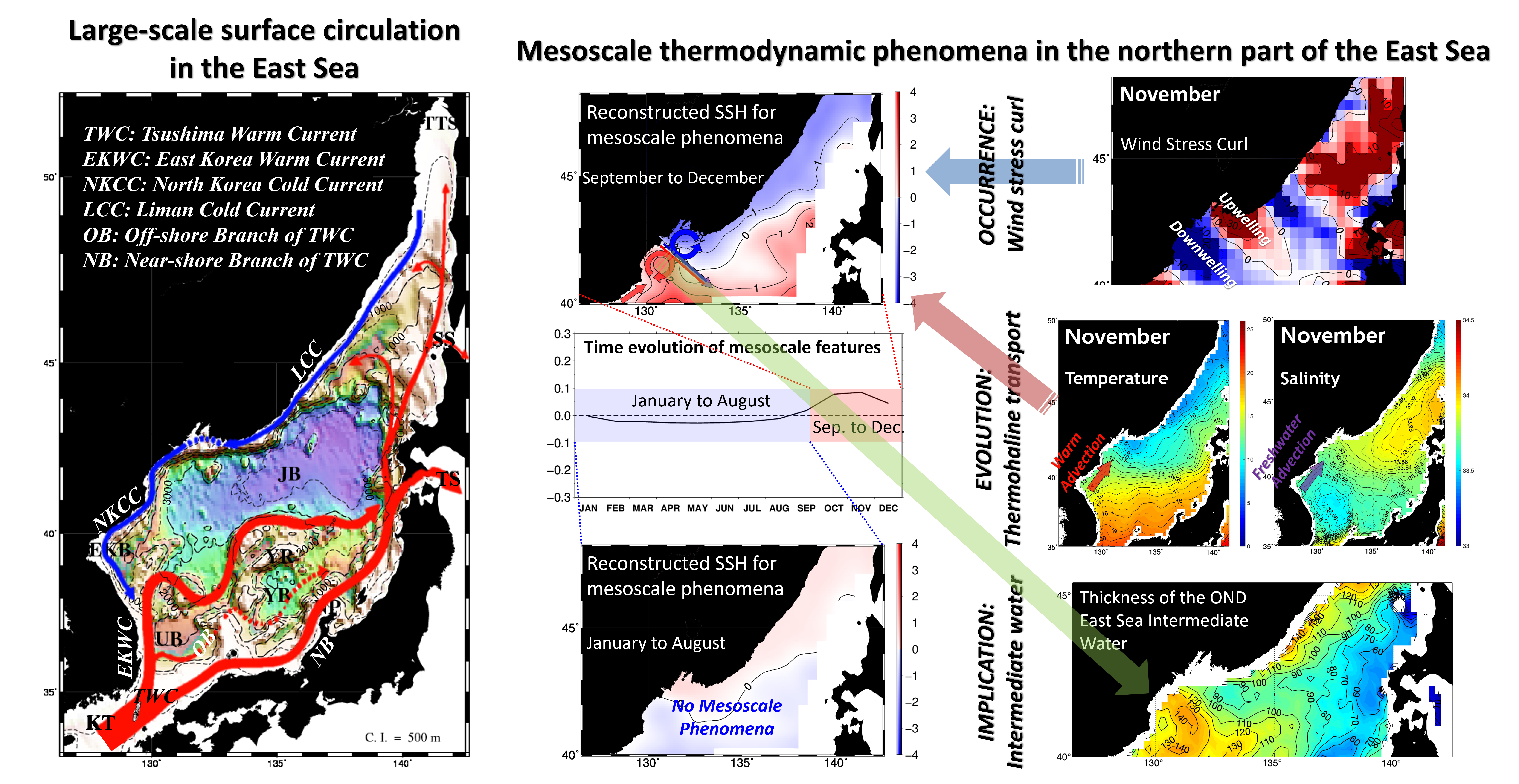
Occurrence and Evolution of Mesoscale Thermodynamic Phenomena in the Northern Part of the East Sea (Japan Sea) Derived from Satellite Altimeter Data

1
Department of Earth and Marine Science, College of Ocean Sciences, Jeju National University, Jeju 63243, Korea
2
Operational Systems Development Department, National Institute of Meteorological Sciences, Seogwipo 63568, Korea
*
Author to whom correspondence should be addressed.
Remote Sens. 2021, 13(6), 1071; https://doi.org/10.3390/rs13061071
Submission received: 19 January 2021 / Revised: 5 March 2021 / Accepted: 8 March 2021 / Published: 11 March 2021

Abstract

:
Based on satellite measurements and oceanic reanalysis data, it has been possible to investigate the spatiotemporal variability of the mesoscale phenomena in the northern part of the East Sea (NES) where direct observations of currents and hydrographical conditions are scarce. For the first time, this study identifies the detailed spatiotemporal structure of the mesoscale features in the NES and the mechanism of its occurrence and evolution, which have important consequences on the distribution of the intermediate water masses in the East Sea. Here, we show that mesoscale thermodynamic phenomena in the northwestern region of the East Sea are characterized by a dipole structure associated with positive and negative sea surface height anomalies. These result in a strong thermal gradient between the seasonally non-persistent anomalies, which emerge and strengthen during late fall and early winter. In contrast to the previous finding of the relationship between winter monsoon winds and mesoscale features in the NES, we found that this relationship is crucial only to the emergence of the mesoscale phenomena. Consequently, we present a new perspective on the evolution mechanism of the mesoscale features in the NES. Of direct significance to the present study, thermohaline transport into the northwestern region of the East Sea regulates the strengthening and weakening of mesoscale features in the NES. Wind forcing may contribute to the emergence of the mesoscale features in the NES and then the intensification of the mesoscale activities is attributed to the intrusion of warm and fresh surface water advected from the southern part of the East Sea.

Graphical Abstract

1. Introduction

Oceanic mesoscale features impact on the overlying atmosphere through thermodynamic processes, which are driven by the sea surface temperature (SST) anomalies associated with the oceanic mesoscale field [1,2,3,4,5]. Moreover, the mesoscale features developed by strong air–sea interaction also play a significant role in delivering the atmospheric forcing into the stratified ocean interior. They have an important effect on the formation and propagation of intermediate and deep waters [6]. Since the interior waters reflect the weather and climate conditions when the water masses are generated, it is important to understand the variabilities of the interior waters, generated through mesoscale processes, in a rapidly-varying climate system [7,8].
The East Sea (ES), which is a small-enclosed marginal sea of the Northwest Pacific, can be regarded as a miniature ocean because its circulation system and hydrography are similar to those of the major ocean basins (Figure 1); sort of cyclonic and anticyclonic gyre systems bounded by the Subpolar Front (SPF), a western boundary current that separates from the coast and forms the SPF, deep water formation by deep convection, and mesoscale eddies and fronts [9,10,11,12]. Major oceanographic features in the ES are inflow and outflow system at the upper layer through the straits [13,14], the SPF [15,16,17], vigorous eddies [18,19,20,21,22,23,24,25], and its own ventilation system to generate anomalous cold and high oxygen deep and bottom waters [26,27]. In particular, the presence of mesoscale eddies in the south and north regions of the ES is an important physical features since the mesoscale phenomena play important roles in ventilating intermediate depths and water mass transformation of the ES [27,28,29,30].
The ES characteristics have been investigated for several decades and are well-documented in many previous studies (e.g., [31] and references therein). Nevertheless, so far, most of these studies focused on the southern part of the ES (i.e., the Tsushima Warm Water region). This is due to the relatively abundant surveys carried out in this region. In contrast, the in situ measurements in the subpolar region have been restricted and direct observations of currents and hydrographical conditions are scarce in the northwestern region of the ES. In particular, there is barely any continuously observed data for a long enough period to investigate the variability of the northern part of the ES (hereafter referred to as NES). However, in the last few decades, owing to the advent and continuous operation of satellite observations and improvement of remote sensing techniques, significant progress has been made in monitoring global ocean surface variations, e.g., [32,33]. It gives a possibility to explore the spatiotemporal variability of NES dynamics. Particularly, empirical orthogonal function (EOF) analysis of sea surface height (SSH) measured by satellite altimetry was used in Kim and Yoon [33] to investigate the upper layer circulation in the NES. They showed that it is characterized by a basin-wide cyclonic circulation, which has significant semi-annual variations strengthening in summer and winter.
Meanwhile, mesoscale features besides the basin-wide cyclonic circulation in the NES were reported by several researchers [34,35,36,37,38]. Based on observations, they showed an anticyclonic eddy that induces a northward coastal current reversal along the North Korean coast and a northwestern thermal front (NWTF) south of Vladivostok during wintertime. Mesoscale eddies and fronts play an essential role in determining the upper pycnocline water properties. In particular, the mesoscale phenomena originating in the NES during winter play a crucial role in producing intermediate and deep waters in the ES [28,29,30,31,39]. Therefore, mesoscale phenomena in the NES are crucial to our understanding of the ES response to global climate change [40,41,42,43]. Although the previous studies report the presence of mesoscale phenomena in the NES, the detailed spatiotemporal variability of the mesoscale features limited by short-term observations. Consequently, the understanding of the mechanism for the evolution of the mesoscale phenomena has been limited as well.
In the present study, we examine and identify the detailed spatiotemporal structure of the mesoscale features in the NES and its seasonality. Furthermore, for the first time, the mechanism of its occurrence and evolution is investigated using continuous observations over a long period (i.e., 1993–2017).

2. Data and Method

2.1. Data Description

In this study, delayed-time level 4 gridded multi-satellite sea level anomalies data with a spatial resolution of 1/4° in latitude and longitude provided by Archiving, Validation and Interpretation of Satellite Oceanographic data (AVISO) are employed to estimate the properties of mesoscale features in the NES. The gridded products are generated by the Ssalto multimission ground segment/Data Unification and Altimeter Combination System (SSALTO/DUACS). The product already includes all of standard corrections to the altimeter data such as tropospheric and ionospheric corrections, corrections for tidal signals and invers barometer response, and sea state bias correction. Other corrections and preprocessing steps applied to the data are detailed in [44]. These data are publicly available through the Copernicus Marine Environment Monitoring Service (CMEMS). Monthly sea level anomaly data that cover the ES basin from January 1993 to December 2017 are used in this study.
Furthermore, to understand the mechanism of occurrence and evolution of the mesoscale phenomena in the NES, we used surface winds derived from the Cross-Calibrated Multi-Platform (CCMP) project and SST from the Operational Sea Surface Temperature and Sea Ice Analysis (OSTIA) dataset. The CCMP wind is 6-hourly gridded analysis data on ocean surface winds at a horizontal resolution of 25 km and produced using a combination of inter-calibrated satellite data from numerous microwave radiometers and microwave scatterometers and in situ data from moored buoys [45,46]. The CCMP product provided a consistent, gap-free long-term period of ocean surface wind fields at the height of 10 m above sea level per day from July 1987 through December 2017. The CCMP wind field data have been widely used due to its accurate capture of offshore winds [47,48]. The SST observations from the OSTIA are determined using several satellite data together with in situ observations. The analysis is performed using the optimal interpolation scheme and is produced daily on a 1/20° Cartesian grid [49,50].
Finally, to investigate the linkage between the mesoscale features and surface layer circulation, we used HYbrid Coordinate Ocean Model and the Navy Coupled Ocean Data Assimilation (HYCOM-NCODA) global reanalysis data, which is a daily eddy-resolving ocean analysis dataset with a resolution of 1/12°. The comparison between observational and oceanic reanalysis data provides insight into the evolution of spatial and temporal patterns of mesoscale features in the NES.
All datasets used in this study are monthly mean products, covering the period from 1993 to 2017.

2.2. Analysis Method

The characteristics of spatial structure and temporal variation of mesoscale features in the NES were described through an EOF analysis of monthly SSHs measured by satellite altimeters for 26 years. EOF technique is widely used in the field of oceanography and meteorology where long time series data are available and has proven to be a powerful tool for resolving physical processes in both fields [51,52,53,54,55]. EOF analysis utilized in this study was based on that applied by Kim and Yoon [8], wherein the covariances were calculated by deviations from the spatial mean of each temporal components.
The variation of the surface current pattern in the NES examined by EOF analysis using the SSH over the entire ES may be strongly influenced by the considerable seasonal variation of the surface circulation in the southern part of the ES. For this reason, EOF analysis was performed using SSHs only over the NES as a region which is not directly affected by the behavior of the Tsushima Warm Current (TWC) coming into the ES that has a considerable seasonal variation (black dashed lines in Figure 1).
Moreover, to explore potential associations between the mesoscale features and surface circulation, we perform and compare composite analysis that is recognized as a simple and effective tool for the identification of the conditions observed during specific states [56]. In this study, composite maps for temperature, salinity and current in the surface layer are calculated for enhanced and weakened mesoscale activities in the NES based on the temporal evolution of the first EOF of the SSH. The years when the normalized temporal evolution values of the EOFs are greater than 1.0 or less than −1.0 standard deviations, are selected to make the composite analysis. We calculate composites of October–November–December (OND) anomalies, when the mesoscale features are manifested, as a deviation from the OND climatology. Additionally, two-tailed student t-test using the Monte Carlo procedure was utilized to test the significance of the anomalies at the 95% confidence level.

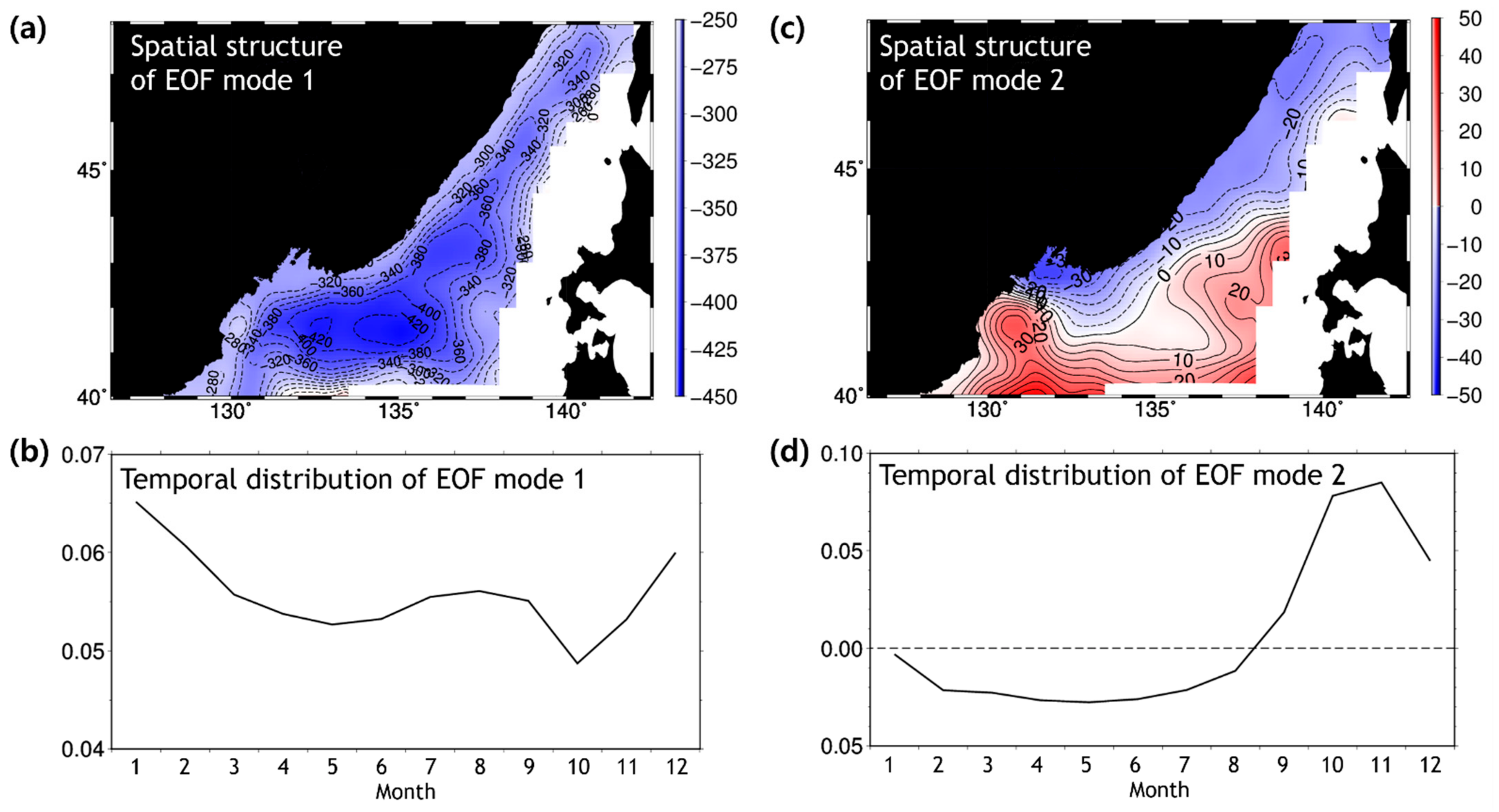
3. Variability of Mesoscale Phenomena in the NES

The first three EOF modes of the SSH variation over the NES contain about 65.7%, 9.8%, and 4.8% of the total variance, respectively. The EOF modes 1 and 2 together explain approximately 75% of the total variance and the spatiotemporal structures of the first two EOF modes are shown in Figure 2. The spatial distribution of the first EOF mode shows that negative values occupy the entire NES with a minimum in the central NES (Figure 2a) and the temporal variation of the mode 1 has a semi-annual variation, indicating maximum values in winter and summer (Figure 2b). The result of the EOF mode 1 implies that the horizontal gradients of spatial distribution become strong during winter and summer. Therefore, the upper layer circulation in the NES is characterized by a large basin-wide cyclonic circulation with significant semi-annual seasonal variation which is strengthened in summer and winter, reconfirming the findings from Kim and Yoon [33].
The spatial distribution and temporal variation of the second EOF mode mainly correspond to the mesoscale variations in the northwestern region of the ES (Appendix A). In the spatial distribution of mode 2, a dipole structure is identified: the oscillations with positive values in the south of the Tumen River mouth (130.5°E, 41.5°N) and oscillations with negative values in the south of Vladivostok in September–December (Figure 2c). The dipole mode is associated with positive and negative SSH anomalies, which reflect warm and cold eddies, resulting in a strong thermal gradient (i.e., the NWTF) between the eddies. The temporal variation of mode 2 has maximum values from October to December and low negative values in the warm period. This finding suggests that the mesoscale features in the NES are not seasonally persistent but manifest in late fall and early winter (Figure 2d).
The results of EOF analysis indicate that, besides the large cyclonic circulation, the current system in the coastal region along the North Korean coast is replaced by anticyclonic flow during October to December, which induces a northeastward coastal reversal. This is confirmed by the trajectory of the ARGOS buoys deployed in July, 1994 during the Circulation Research of the East Asian Marginal Seas (CREAMS ’94) summer cruise (see Figure 2a in Yoon et al. [36]). The northward reversal of coastal current reveals that relatively warm and fresh-water from the southern region of the ES flow into the western side of the NWTF during that time. The intrusion of warm and fresh-water along the North Korean coast could be a critical factor in intensifying the mesoscale features in the NES. Moreover, it implies that a strong thermal gradient develops off the Tumen River mouth between the negative and positive anomalies in late fall and early winter. This thermal gradient is accompanied by a cold anomaly in the eastern side and a weak warm anomaly in the western side, which is supported by in situ temperature measurements for January, 1986 [34] and climatological SST from OSTIA (Figure 3a).

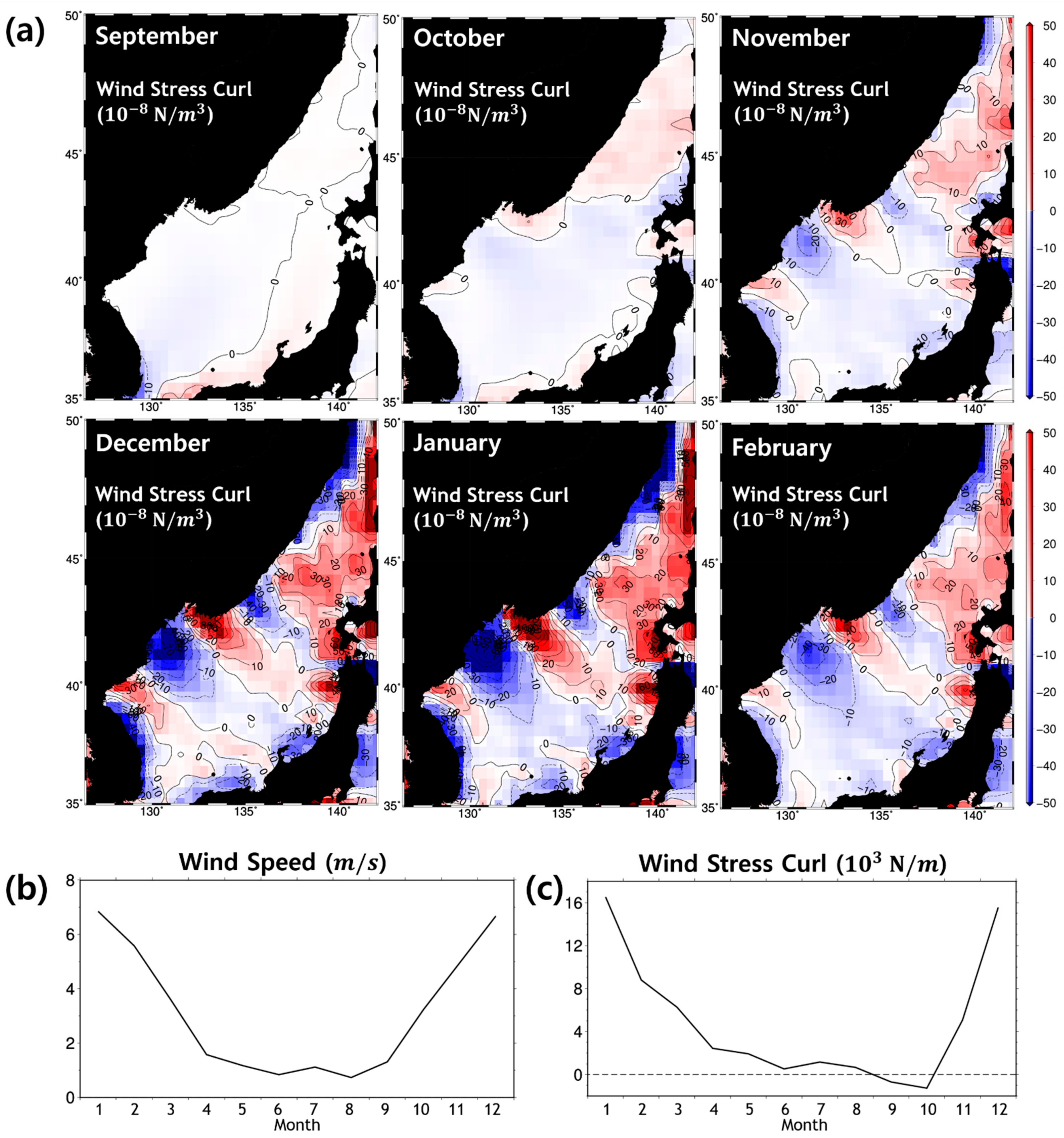
4. Occurrence of Mesoscale Features in the NES

Atmospheric forcing can be an essential source of mesoscale variability in the ocean [57]. In particular, atmospheric disturbances, such as cold air outbreak and tropical cyclones, significantly impact oceanic mesoscale features [58]. Previous studies have shown that mesoscale phenomena in the NES may be closely related to atmospheric submesoscale disturbances south of Vladivostok [35,36,38]. Namely, the northwesterly cold-air outbreak passing through the orographic gap near Vladivostok due to the East Asia winter monsoon is accompanied by a dipole of wind stress curl to the south of Vladivostok (Figure 4a), which exerts a significant influence on the circulation north of the SPF in the ES. Our results also show that the location of the dipole structure of the mesoscale eddies in the NES exactly coincides with the dipole of the wind stress curl, which develops south of Vladivostok in winter. The dipole wind stress curl structure generates cold and warm anomalies through wind-induced upwelling and downwelling off the coast due to Ekman dynamics. The cold SST anomaly is generated by the Ekman divergence due to the positive wind-stress curl (upwelling) off Vladivostok. On the other hand, a warm anomaly appears below the negative wind stress curl in the process of the downwelling imposed by the anticyclonic vortex. Consequently, a thermal front is formed between these cold and warm anomalies.
Furthermore, as reported in previous studies (e.g., [59,60,61]), the anticyclonic flows accompanied by northward coastal current reversal are generated by a negative wind stress curl. It may bring relatively warm and fresh water from the southern area into the downwelling region. These features are demonstrated by horizontal distributions of the climatological monthly mean temperature and salinity in the surface layer from reanalysis data averaged from 1993 to 2017 (Figure 3b,c) and the results of EOF analysis. This indicates that wind stress forcing controls the mesoscale features in the NES.
Interestingly, unlike wind speed, the wind stress curl integrated in the NES region decreases gradually until October (it has negative values in September and October). Then, it begins developing rapidly in November and peaks in December–January (Figure 4b,c). The timing of the occurrence of the mesoscale phenomena can be explained as follows: as suggested in previous studies [33,62] a large basin-wide cyclonic circulation in the NES is generated and strengthened by the positive wind stress curl, which successively affects the corresponding sea areas. Accordingly, in fall, when the wind stress curl integrated over the NES is the lowest (i.e., negative value), the basin-wide cyclonic circulation in the NES attains its weakest intensity for the year (see Figure 5c and Figure 12a in Kim and Yoon [33]). Consequently, the mesoscale structure can be subject to a relatively strong variability associated with the prevailing negative wind stress curl over the corresponding region in that period.
Accordingly, winter monsoon winds may play a significant role in the generation and evolution of the mesoscale phenomena in the NES. Previous studies have also attributed the occurrence and evolution of the mesoscale features in the NES to the strong northwesterly winds in winter. It is worth noting, however, that there is a discrepancy between the maximum timing of the mesoscale features and wind forcing. The winds lag behind the mesoscale features by approximately two months. The mesoscale features in the NES reach a maximum in October–November (Figure 2d), whereas the wind forcing has maximum values in December–January due to intense winter monsoons (Figure 4b,c). As Park et al. [35] note, the mesoscale front can be determined by differential surface cooling and the difference in thermal inertial between the downwind and off-wind areas. These facts reveal that a different mechanism, except for wind forcing, may be more critical in the evolution and strengthening of mesoscale features in the NES.

5. Evolution of Mesoscale Features in the NES

Figure 5 shows the year-to-year variations in the mesoscale features in the NES, negative wind stress curl over the region with positive SSH anomalies, and SST difference between the regions with positive and negative SSH anomalies. They are all time-series of three months mean (i.e., OND mean when the mesoscale features are manifested in the NES) of each value from 1993 to 2017. The wind stress curl and the SST difference were spatially averaged over each corresponding region (indicated by red and blue boxes in Figure 1). As shown in Figure 5, the results show a remarkably different interannual variability in the temporal structures, between the intensities in the mesoscale features and wind stress curl in the NES. During the period 1993–2017, the mesoscale phenomena in the NES was weak in 2005 when the wind stress curl was the strongest. Conversely, in 2003 when wind forcing was relatively weak, it intensified considerably. This finding indicates that the variability in wind forcing which regarded as driving the mesoscale features in the NES, is poorly correlated with the variability of mesoscale features on interannual timescales (the correlation coefficient is 0.22 for the 25-year period from 1993 to 2017) as well as seasonal timescale. In contrast, the mesoscale features in the NES highly correlates with the SST difference between the regions with positive and negative SSH anomalies (the correlation coefficient is 0.74 for the 25-year period). Thus, the SST gradient between the dipole regions faithfully reflects the dominant variability in mesoscale features in the NES.
The SST is locally determined by a balance between the surface heat flux, horizontal diffusion, entrainment from below the mixed layer resulting from imposed winds, and lateral heat advection by ocean currents. The results of EOF analysis, as well as satellite SST data and surface temperature from reanalysis data, show that the thermal gradient between positive and negative oscillations is the largest in OND rather than in December–January when the cold and dry northwesterly winds are the strongest. The horizontal distributions of the SST observed by satellite, and surface temperature and salinity from reanalysis data, show that warm and fresh southern water flows into the northwestern part of the ES in OND, thus resulting in a strong front together with the relatively cold and salty water in the region of the positive wind stress curl (Figure 3). However, the development of the front has been restricted since January due to the strong wind mixing and intense surface cooling on both sides of the front in winter.
To explore potential associations between the mesoscale features and surface layer circulation, the composite maps for temperature, salinity, and current at 20 m depth were calculated using HYCOM reanalysis data for enhanced and weakened mesoscale activities in the NES based on the temporal evolution of the second EOF mode of the SSH (Figure 5; strong years: 1999, 2003, 2007, 2016, 2017; weak years: 1993, 1995, 1997, 2012, 2013). Figure 6 shows the average anomalous temperature, salinity, and current conditions for the mesoscale activities.
The composite maps suggest that the enhanced mesoscale activities in the NES are closely associated with the anomalous warm and fresh water in the northwestern part of the ES, accompanied by northeastward current anomalies along the North Korean coast. In contrast, the southwestward current anomalies along the coast and anomalous cold and salty conditions in the northwestern region of the ES are related to weakened mesoscale features. Accordingly, to identify the contribution of the lateral advection of warm and fresh waters in the upper layer (i.e., surface to 200 m depth) to the intensification of the mesoscale features in the NES, we estimated the heat ( H T ) [63] and freshwater ( F T ) [64] transports into the northwestern region of the ES (passing through 40°N, between 128°E and 130°E; indicated by the yellow line in Figure 1) during the time of year when the mesoscale features in the NES are manifested as follows:
H T = ρ w c p T v d x d z
F T = v S S 0 S 0 d x d z
where ρ w is the density of seawater, c p is the specific heat capacity at constant pressure, T and S are the upper layer temperature and salinity, respectively, and v is the meridional velocity. S 0 is a reference salinity and equal to 34.09 psu (mean salinity of the ES). The positive (negative) value of each transport indicates that the transport is northward (southward) across the line.
The interannual variations of the OND heat and freshwater transport into the northwestern region of the ES are shown in Figure 7. This clarifies the effect of thermohaline transport on the variability of the mesoscale features in the NES. There is a significant relationship between the mesoscale features in the NES and thermohaline transport, within and across seasons and interannually (the correlation coefficients are 0.66 for heat transport and 0.67 for freshwater transport). The northwestern region of the ES experienced considerable lateral heat and freshwater inflow from the south when the mesoscale activities were enhanced (e.g., in 2003). On the contrary, weakening of mesoscale features of the NES entails a considerably larger southward thermohaline transport across 40°N (e.g., 2012). Consequently, the lateral heat and freshwater transport into the northwestern region of the ES, carried out by oceanic currents, plays a critical role in strengthening and weakening of the mesoscale features in that region. This is the main finding of this study.

6. Summary and Implications

Occurrence and temporal evolution of the mesoscale features in the NES are investigated using EOF analysis of the SSH obtained from satellite observations for 25 years (i.e., 1993–2017). Our results show that, besides the large basin-wide cyclonic circulation, the mesoscale features in the northwestern region of the ES are characterized by a dipole mode associated with warm and cold eddies, thus resulting in a strong thermal gradient between the seasonally non-persistent eddies, which emerged and strengthened during late fall and early winter.
Previous studies show that the mesoscale phenomena in the NES may be closely related to a dipole of wind stress curl to the south of Vladivostok in winter. Consistently, our results show that the wind stress curl and mesoscale features in the NES estimated using the altimeter data, exhibit remarkably similar spatial structure throughout the observation period. This is likely to imply the wind stress forcing considerable controls on the mesoscale features in the NES. However, there is a discrepancy between the maximum timing of mesoscale features and wind forcing. Furthermore, our results show that the mesoscale features are poorly correlated with wind forcing on interannual timescales (r = 0.22). To investigate the evolution mechanism of the mesoscale features, we evaluate the influence of heat and freshwater transport into the northwestern region of the ES, as implied by the composite maps for anomalous temperature, salinity, and currents. The results reveal a strong relationship between the mesoscale activities and thermohaline transport, within and across seasons and interannually. The thermohaline transport into the northwestern region of the ES is shown to regulate the strengthening and weakening the mesoscale features at the study area. This is a significant finding of this study.
Based on these findings, we present a new perspective on the evolution of mesoscale features in the NES, using continuous observations over a long period. We demonstrate, for the first time, that the mesoscale features in the NES are not seasonally persistent, however, manifesting in late fall and early winter. Moreover, oceanic thermohaline transport, rather than wind forcing, is more important in the evolution of the mesoscale features. Wind forcing may contribute to the development of the mesoscale features in the NES, while the intensification of the mesoscale activities is attributed to the intrusion of warm and fresh surface water advected from the southern part of the ES in fall.
The mesoscale features generated by strong air–sea interaction, play a significant role in delivering the atmospheric forcing into the stratified ocean interior. Therefore, the mesoscale variability has an essential effect on the formation and propagation of intermediate and deep waters. Moreover, it is found that in the ES, low-salinity water ventilated at the sea surface north of the SPF because of intense vertical mixing, is elongated toward the subsurface south of the SPF below the TWC. This is the East Sea Intermediate Water (ESIW), which is the main salinity minimum water mass with high oxygen content, corresponding to the North Pacific Intermediate Water [65]. Since the intermediate water reflects the weather and climate conditions when the water masses are generated, the variability of the intermediate water which is generated through the mesoscale processes is significant in climate change and ocean circulation.
Recently, Park and Lim [39] investigated the formation area of the ESIW and the temperature and salinity structure of its formation period using data collected by Argo floats. They suggested that the ESIW is formed in the northwestern part of the ES (40–42°N, 130–133°E), where a strong negative surface wind stress curl resides during winter. The region of the ESIW formation perfectly overlaps the region with a positive SSH anomaly in EOF mode 2 (Figure 2c and Figure 8a). The annual variation in the ESIW thickness for OND indicates that the ESIW thickness and the mesoscale features in the NES fluctuate coherently (Figure 8b). The mesoscale phenomena originating in the NES would play a crucial role in producing intermediate water in the ES. Our results provide important insights for the long-term variability of interior water masses together with the change in oceanic and atmospheric circulation by understanding the long-term variability of mesoscale features in global climate change. Recently, a number of studies have reported the decadal and interannual variabilities of intermediate and deep water in the ES [40,41,42,43]. They found contrasting intermediate and deep water formation and the ES’s meridional overturning (thermohaline) circulation in the late 1990s and early 2000s. The temporal evolution of the mesoscale phenomena in the NES also shows consistent time evolution with previous findings reported recently. Although not investigated in this study, it is a fascinating subject for future work.

Author Contributions

Conceptualization, T.K.; methodology, T.K. and J.-H.M.; validation, T.K. and H.-J.J.; formal analysis, T.K., H.-J.J. and J.-H.M.; data curation, H.-J.J.; writing—original draft preparation, T.K.; writing—review and editing, T.K. and J.-H.M.; visualization, T.K. and H.-J.J.; supervision, T.K. and J.-H.M. All authors have read and agreed to the published version of the manuscript.

Funding

This research was funded by Basic Science Research Program through the National Research Foundation of Korea (NRF) funded by the Ministry of Education, Korea (NRF-2020R1I1A1A01053137). H.-J.J. was supported by the Korea Meteorological Administration Research and Development Program “Development of Marine Meteorology Monitoring and Next-generation Ocean Forecasting System” under Grant (KMA2018-00420). J.-H.M. was supported by the National Research Foundation of Korea (NRF) funded by the Korea government (MSIP) (NRF-2019R1A2C1003206).

Institutional Review Board Statement

Not applicable.

Informed Consent Statement

Not applicable.

Data Availability Statement

Data available in a publicly accessible repository that does not issue DOIs. The Ssalto/Duacs altimeter products and OSTIA SST were produced and distributed by the Copernicus Marine and Environment Monitoring Service (CMEMS) (http://www.marine.copernicus.eu, accessed on 21 August 2018). CCMP Version-2.0 vector wind analyses were produced by Remote Sensing Systems. The data are available at www.remss.com, accessed on 21 August 2018. HYCOM reanalysis data is available at https://www.hycom.org/, accessed on 21 August 2018.

Acknowledgments

T.K. expresses his gratitude to Jong-Hwan Yoon for his valuable comments and suggestions on this work. H.-J.J. would like to thank S.H. Choo for his great coordination to collect data for this research. The authors gratefully acknowledge the editor and the seven anonymous reviewers for their insightful comments and contributions to the manuscript.

Conflicts of Interest

The authors declare no conflict of interest.

Appendix A

It is a critical issue for the present study whether the spatial distribution of the second EOF mode shows the mesoscale variations in the NES. Previous studies [15,66] report that there is a large difference in the spatial pattern of eddy kinetic energy (EKE), which indicates eddy activity, in the ES. Small eddy energy was found in the northern cold water regime and large eddy energy in the southern warm water regime. In particular, eddy activity in the NES is strong in the northwestern region, whereas eddy energy is considerably weak in the northeastern ES. To identify that the second EOF mode corresponds to the variability of mesoscale eddy dynamics in the NES, the EKE in the ES is calculated. The EKE is estimated from gridded sea level anomaly data from AVISO by making the geostrophic assumption.
E K E = 1 2 U g 2 + V g 2
U g = g f Δ η Δ y
V g = g f Δ η Δ x
where U g and V g denote the zonal and meridional geostrophic velocity anomalies, f is the Coriolis parameter, η is sea level anomaly, and Δx and Δy are the distances in longitude and latitude (1/4° in AVISO).
Figure A1 displays the spatial patterns of climatological monthly mean EKE in the ES. In accordance with the results of previous studies, the region of high intensity corresponds to the southern part of the ES, whereas it is relatively low in the cold water region that is the study area. Nevertheless, in the northwestern region of the ES, in the south of Vladivostok, significant energy is observed from September to January (stronger in OND). On the other hand, the lowest energies are observed in the northeastern part of the ES throughout the year. The characteristics of mesoscale eddies in the NES are also demonstrated by Lee et al. [66] in which energetic mesoscale eddies in the ES associated with strong mesoscale variability were statistically characterized by analyzing satellite altimeter data and in situ observations.
Figure A1. Horizontal distributions of climatological monthly mean eddy kinetic energy ( cm 2 / s 2 ) in September—February averaged from 1993 through 2017.
Remotesensing 13 01071 g0a1
The spatial pattern and temporal variation of the mode 2 are consistent to that of the EKE in the NES. These distributions confirm the results of EOF analysis using SSH over the NES that the spatial distribution and temporal variation of the second EOF mode mainly correspond to the mesoscale variations in the northwestern region of the ES.

References

  1. Wallace, J.M.; Mitchell, T.P.; Deser, C. The influence of sea surface temperature on surface wind in the eastern equatorial Pacific: Seasonal and interannual variability. J. Clim. 1989, 2, 1492–1499. [Google Scholar] [CrossRef]
  2. Minobe, S.; Kuwano-Yoshida, A.; Komori, N.; Xie, S.-P.; Small, R.J. Influence of the Gulf Stream on the troposphere. Science 2008, 452, 206–209. [Google Scholar] [CrossRef]
  3. Small, R.J.; de Szoeke, S.P.; Xie, S.P.; O’Neill, L.; Seo, H.; Song, Q.; Cornillon, P.; Spall, M.; Minobe, S. Air–sea interaction over ocean fronts and eddies. Dyn. Atmos. Ocean 2008, 45, 274–319. [Google Scholar] [CrossRef]
  4. Chelton, D.B.; Xie, S.-P. Coupled ocean-atmosphere interaction at oceanic mesoscales. Oceanography 2010, 23, 52–69. [Google Scholar] [CrossRef]
  5. Lin, P.; Lui, H.; Ma, J.; Li, Y. Ocean mesoscale structure–induced air–sea interaction in a high-resolution coupled model. Atmos. Ocean. Sci. Lett. 2019, 12, 98–106. [Google Scholar] [CrossRef] [Green Version]
  6. Lee, C.M.; Thomas, L.N.; Yoshikawa, Y. Intermediate water formation at the Japan/East Sea subpolar front. Oceanography 2006, 19, 110–121. [Google Scholar] [CrossRef] [Green Version]
  7. Levitus, S.; Antonov, J.I.; Boyer, T.P.; Stephens, C. Warming of the world ocean. Science 2000, 287, 2225–2229. [Google Scholar] [CrossRef] [Green Version]
  8. Wong, A.P.S.; Bindoff, N.L.; Church, J.A. Large-scale freshening of intermediate waters in the Pacific and Indian Oceans. Nature 1999, 400, 440–443. [Google Scholar] [CrossRef]
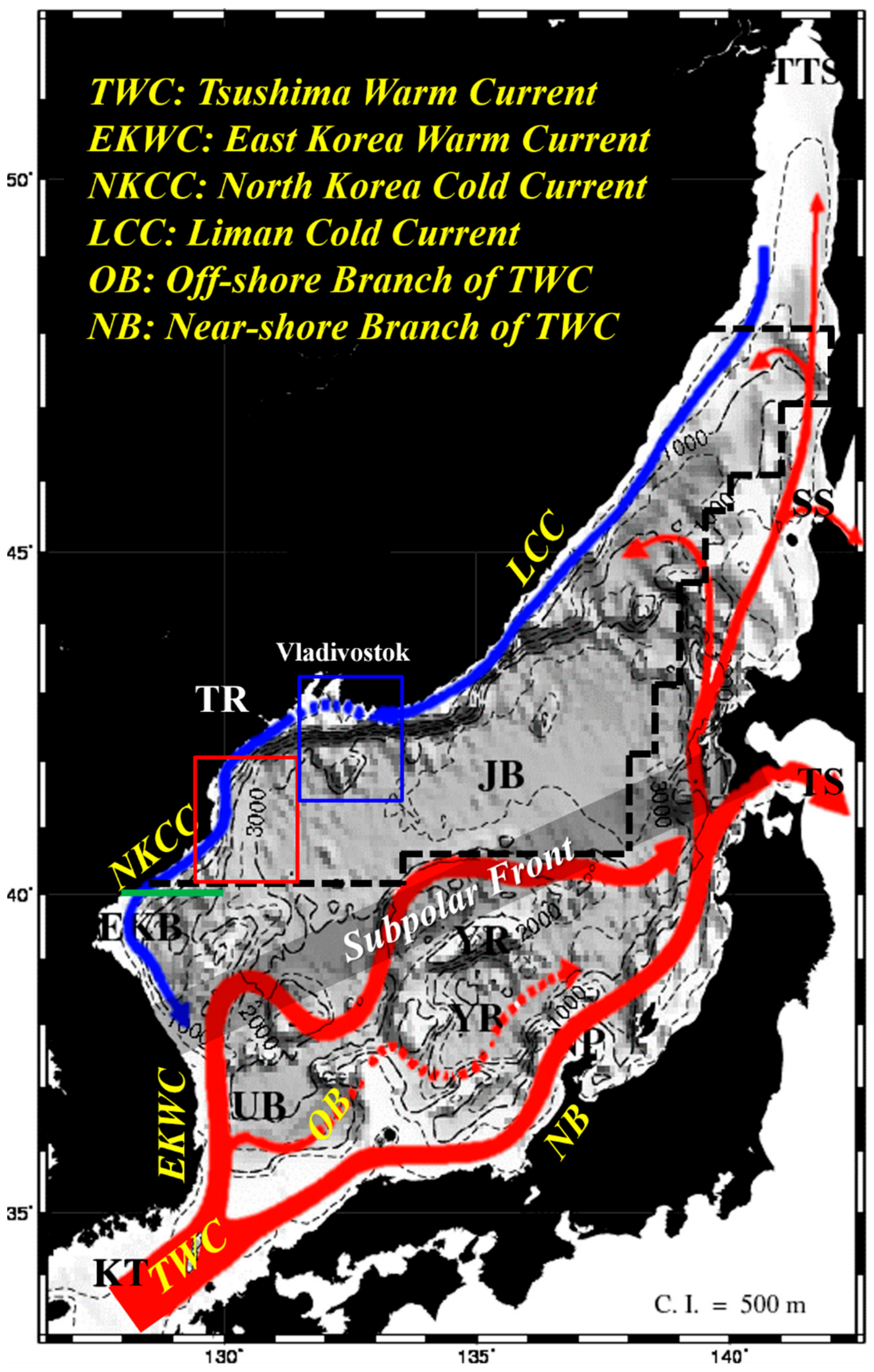
  9. Park, K.-A.; Park, J.-E.; Choi, B.-J.; Byun, D.-S.; Lee, E.-I. An oceanic current map of the East Sea for science textbooks based on scientific knowledge acquired from oceanic measurements. J. Korean Soc. Oceanogr. 2013, 18, 234–265. [Google Scholar] [CrossRef]
  10. Ichiye, T. Some problems of circulation and hydrography of the Japan Sea and the Tsushima Current. In Ocean Hydrodynamics of the Japan and East China Seas; Ichiye, T., Ed.; Elsevier: Amsterdam, The Netherlands, 1984; Volume 39, pp. 15–54. [Google Scholar]
  11. Senjyu, T. The Japan Sea Intermediate Water; Its Characteristics and Circulation. J. Oceanogr. 1999, 55, 111–122. [Google Scholar] [CrossRef]
  12. Kim, K.; Kim, K.R.; Min, D.H.; Volkov, Y.; Yoon, J.-H.; Takematsu, M. Warming and structural changes in the East (Japan) Sea: A clue to future changes in global oceans? Geophy. Res. Lett. 2001, 28, 3293–3296. [Google Scholar] [CrossRef]
  13. Morimoto, A.; Yanagi, T. Variability of sea surface circulation in the Japan Sea. J. Oceanogr. 2001, 57, 1–13. [Google Scholar] [CrossRef]
  14. Lee, D.K.; Niiler, P.P. The energetic surface circulation patterns of the Japan/East Sea. Deep Sea Res. Part II 2005, 52, 1547–1563. [Google Scholar] [CrossRef]
  15. Isoda, Y. Interannual SST variations to the north and south of the polar front in the Japan Sea. La Mer 1994, 32, 285–293. [Google Scholar]
  16. Mooers, C.N.K.; Bang, I.; Sandoval, F.J. Comparison between observation and numerical simulations of Japan (East) Sea flow and mass fields in 1999 through 2001. Deep Sea Res. Part II 2005, 52, 1639–1661. [Google Scholar] [CrossRef]
  17. Park, K.-A.; Ullman, D.S.; Kim, K.; Chung, J.Y.; Kim, K.-R. Spatial and temporal variability of satellite-observed subpolar front in the East/Japan Sea. Deep Sea Res. Part I 2007, 54, 453–470. [Google Scholar] [CrossRef]
  18. An, H.S. On the cold water mass around the southeast coast of Korean Peninsula. J. Oceanol. Soc. Korea 1974, 9, 10–18. [Google Scholar]
  19. Cho, K.-D.; Bang, T.-J.; Shim, T.-B.; Yu, H.-S. Three dimensional structure of the Ulleung warm lens. Bull. Korean Fish. Soc. 1990, 23, 323–333. [Google Scholar]
  20. Kim, K.; Kim, K.-R.; Chung, J.-Y.; Yoo, H.-S.; Park, S.-G. Characteristics of physical properties in the Ulleung Basin. J. Korean Soc. Oceanogr. 1991, 31, 155–163. [Google Scholar]
  21. Isoda, Y. Warm eddy movements in the eastern Japan Sea. J. Oceanogr. 1994, 50, 1–15. [Google Scholar] [CrossRef] [Green Version]
  22. Lie, H.-J.; Byun, S.K.; Bang, I.K.; Cho, C.H. Physical structure of eddies in the southwestern East Sea. J. Oceanol. Soc. Korea 1995, 24, 63–68. [Google Scholar]
  23. Chang, K.-I.; Teague, W.J.; Lyu, S.J.; Perkins, H.T.; Lee, D.-K.; Watts, D.R.; Kim, Y.-B.; Mitchell, D.A.; Lee, C.M.; Kim, K. Circulation and currents in the southwestern East/Japan Sea: Overview and review. Prog. Oceanogr. 2004, 61, 105–156. [Google Scholar] [CrossRef]
  24. Shin, H.-R.; Shin, C.-W.; Kim, C.; Byun, S.-K.; Hwang, S.-C. Movement and structural variation of warm eddy WE92 for three years in the Western East/Japan Sea. Deep Sea Res. Part II 2005, 52, 1742–1762. [Google Scholar] [CrossRef]
  25. Mithchell, D.A.; Watts, D.R.; Wimbush, M.; Teague, W.J.; Tracey, K.L.; Book, J.B.; Chang, K.-I.; Suk, M.-S.; Yoon, J.-H. Upper circulation pattern in the Ulleung Basin. Deep Sea Res. Part II 2005, 52, 1617–1638. [Google Scholar] [CrossRef]
  26. Postlethwaite, C.F.; Rohling, E.J.; Jenkins, W.J.; Walker, C.F. A tracer study of ventilation in the Japan/East Sea. Deep Sea Res. Part II 2005, 52, 1684–1704. [Google Scholar] [CrossRef]
  27. Min, D.-H.; Warner, M.J. Basin-wide circulation and ventilation study in the East Sea (Sea of Japan) using chloroflurocarbon tracers. Deep Sea Res. Part II 2005, 52, 1580–1616. [Google Scholar] [CrossRef]
  28. Kim, C.-H.; Yoon, J.-H. A numerical modeling of the upper and the intermediate layer circulation in the East Sea. J. Oceanogr. 1999, 55, 327–345. [Google Scholar] [CrossRef]
  29. Talley, L.D.; Tishchenko, P.; Luchin, V.; Nedashkovskiy, A.; Sagalaev, S.; Kang, D.-J.; Warner, M.; Min, D.H. Atlas of Japan (East) Sea hydrographic properties in summer, 1999. Prog. Oceanogr. 2004, 61, 277–348. [Google Scholar] [CrossRef]
  30. Talley, L.D.; Min, D.-H.; Lobanov, V.B.; Luchin, V.A.; Ponomarev, V.I.; Salyuk, A.N.; Schcerbina, A.Y.; Tishchenko, P.Y.; Zhabin, A.I. Japan/East Sea water masses and their relation to the sea’s circulation. Oceanography 2006, 19, 32–49. [Google Scholar] [CrossRef] [Green Version]
  31. Chang, K.-I.; Zhang, C.-I.; Park, C.; Kang, D.-J.; Ju, S.-J.; Lee, S.-H.; Wimbush, M. Oceanography of the East Sea (Japan Sea); Springer: Cham, Switzerland, 2016; p. 460. [Google Scholar]
  32. Yang, H.; Lohmann, G.; Krebs-Kanzow, U.; Ionita, M.; Shi, X.; Sidorenko, D.; Gong, X.; Chen, X.; Gowan, E.J. Poleward shift of the major ocean gyres detected in a warming climate. Geophys. Res. Lett. 2020, 47, e2019GL085868. [Google Scholar] [CrossRef] [Green Version]
  33. Kim, T.; Yoon, J.-H. Seasonal variation of upper layer circulation in the northern part of the East/Japan Sea. Cont. Shelf Res. 2010, 30, 1283–1301. [Google Scholar] [CrossRef]
  34. Danchenkov, M.A.; Aubrey, D.G.; Feldman, K.L. Oceanography of area close to the Tumannaya river mouth (the Japan Sea). Pacific Oceanogr. 2003, 1, 61–69. [Google Scholar]
  35. Park, K.-A.; Chung, J.; Kim, K. Sea surface temperature fronts in the East (Japan) Sea and temporal variations. Geophys. Res. Lett. 2004, 31, L07304. [Google Scholar] [CrossRef]
  36. Yoon, J.-H.; Abe, K.; Ogata, T.; Wakamatsu, Y. The effects of wind-stress curl on the Japan/East Sea circulation. Deep Sea Res. II 2005, 52, 1827–1844. [Google Scholar] [CrossRef]
  37. Trusenkova, O.; Nikitin, A.; Lobanov, V. Circulation features in the Japan/East Sea related to statistically obtained wind patterns in the warm season. J. Mar. Syst. 2009, 78, 214–225. [Google Scholar] [CrossRef]
  38. Yoon, J.-H.; Kim, Y.-J. Review on the seasonal variation of the surface circulation in the Japan/East Sea. J. Mar. Syst. 2009, 78, 226–236. [Google Scholar] [CrossRef]
  39. Park, J.; Lim, B. A new perspective on origin of the East Sea Intermediate water: Observations of Argo floats. Prog. Oceanogr. 2017, 160, 213–224. [Google Scholar] [CrossRef]
  40. Nam, S.; Yoon, S.-T.; Park, J.-H.; Kim, Y.H.; Chang, K.-I. Distinct characteristics of the intermediate water observed off the east coast of Korea during two contrasting years. J. Geophys. Res. Oceans 2016, 121, 5050–5068. [Google Scholar] [CrossRef]
  41. Yoon, S.-T.; Chang, K.-I.; Nam, S.; Rho, T.; Kang, D.-J.; Lee, T.; Park, K.-A.; Lobanov, V.; Kaplunenko, D.; Tishchenko, P.; et al. Re-initiation of bottom water formation in the East Sea (Japan Sea) in a warming world. Sci. Rep. 2018, 8, 1576. [Google Scholar] [CrossRef] [PubMed]
  42. Lee, E.Y.; Park, K.-A. Change in the Recent Warming Trend of Sea Surface Temperature in the East Sea (Sea of Japan) over Decades (1982–2018). Remote Sens. 2019, 11, 2613. [Google Scholar] [CrossRef] [Green Version]
  43. Han, M.H.; Cho, Y.-K.; Kang, H.-W.; Nam, S. Decadal changes in meridional overturning circulation in the East Sea (Sea of Japan). J. Phys. Oceanogr. 2020, 50, 1773–1791. [Google Scholar] [CrossRef]
  44. CLS. “SSALTO/DUACS Experimental Product Handbook”, SALP-MU-P-EA-23172-CLS, 52 pp. 2020. Available online: https://www.aviso.altimetry.fr/fileadmin/documents/data/tools/hdbk_duacs_experimental.pdf (accessed on 24 November 2020).
  45. Atlas, R.; Hoffman, R.N.; Ardizzone, J.; Leidner, S.M.; Jusem, J.C.; Smith, D.K.; Gombos, D. A cross-calibrated, multiplatform ocean surface wind velocity product for meteorological and oceanographic applications. Bull. Amer. Meteor. Soc. 2011, 92, 157–174. [Google Scholar] [CrossRef]
  46. Wentz, F.J.; Scott, J.; Hoffman, R.; Leidner, M.; Atlas, R.; Ardizzone, J. Remote Sensing Systems Cross-Calibrated Multi-Platform (CCMP) 6-Hourly Ocean Vector Wind Analysis Product on 0.25 Deg Grid, Version 2.0, Remote Sensing Systems. Santa Rosa, CA. 2015. Available online: www.remss.com/measurements/ccmp (accessed on 21 August 2018).
  47. Carvalho, D.; Rocha, A.; Gómez-Gesteira, M.; Silva Santos, C. Comparison of reanalyzed, analyzed, satellite-retrieved and NWP modelled winds with buoy data along the Iberian Peninsula coast. Remote Sens. Environ. 2014, 152, 480–492. [Google Scholar] [CrossRef]
  48. Zheng, C.W.; Pan, J. Assessment of the global ocean wind energy resource. Renew. Sustain. Energy Rev. 2014, 33, 382–391. [Google Scholar] [CrossRef]
  49. Donlon, C.J.; Martin, M.; Stark, J.; Roberts-Jones, J.; Fiedler, E.; Wimmer, W. The operational sea surface temperature and sea ice analysis (OSTIA) system. Remote Sens. Environ. 2012, 116, 140–158. [Google Scholar] [CrossRef]
  50. Good, S.; Fiedler, E.; Mao, C.; Martin, M.J.; Maycock, A.; Reid, R.; Roberts-Jones, J.; Searle, T.; Waters, J.; While, J.; et al. The Current Configuration of the OSTIA System for Operational Production of Foundation Sea Surface Temperature and Ice Concentration Analyses. Remote. Sens. 2020, 12, 720. [Google Scholar] [CrossRef] [Green Version]
  51. Kelly, K.A. The influence of winds and topography on the sea surface temperature patterns over the northern California slope. J. Geophys. Res. 1985, 90, 11783. [Google Scholar] [CrossRef]
  52. Chu, P.C.; Lu, S.H.; Chen, Y.C. Temporal and spatial variabilities of the South China Sea surface temperature anomaly. J. Geophys. Res. 1997, 102, 20937–20955. [Google Scholar] [CrossRef] [Green Version]
  53. Kuo, N.-J.; Zheng, Q.; Ho, C.-R. Response of Vietnam coastal upwelling to the 1997–1998 ENSO event observed by multisensor data. Remote Sens. Environ. 2004, 89, 106–115. [Google Scholar] [CrossRef]
  54. Shaw, P.-T.; Chao, S.-Y.; Fu, L.-L. Sea surface height variations in the South China Sea from satellite altimetry. Oceanol. Acta 1999, 22, 1–17. [Google Scholar] [CrossRef] [Green Version]
  55. Kok, P.H.; Akhir, M.F.; Qiao, F. Distinctive characteristics of upwelling along the Peninsular Malaysia’s east coast during 2009/10 and 2015/16El Niños. Cont. Shelf Res. 2019, 184, 10–20. [Google Scholar] [CrossRef]
  56. Boschat, G.; Simmonds, I.; Purich, A.; Cowan, T.; Pessa, A.B. On the use of composite analyses to form physical hypotheses: An example from heat wave—SST associations. Sci. Rep. 2016, 6, 29599. [Google Scholar] [CrossRef]
  57. Orlanski, I.; Polinsky, L.J. Ocean response to mesoscale atmospheric forcing. Tellus 1983, 35, 296–323. [Google Scholar] [CrossRef] [Green Version]
  58. Kim, T.; Choo, S.-H.; Moon, J.-H.; Chang, P.-H. Contribution of tropical cyclones to abnormal sea surface temperature warming in the Yellow Sea in December 2004. Dyn. Atmos. Ocean 2017, 80, 97–109. [Google Scholar] [CrossRef]
  59. Park, J.-H.; Chang, K.-I.; Nam, S. Summertime coastal current reversal opposing offshore forcing and local wind near the middle east coast of Ko-rea: Observations and dynamics. Geophys. Res. Lett. 2016, 43, 7097–7105. [Google Scholar] [CrossRef] [Green Version]
  60. Park, J.-H.; Nam, S. Causes of Interannual Variation of Summer Mean Alongshore Current Near the East Coast of Korea Derived From 16-Year-Long Observational Data. J. Geophys. Res. Oceans 2018, 123, 7781–7794. [Google Scholar] [CrossRef]
  61. Son, Y.-T.; Park, J.-H.; Nam, S. Summertime episodic chlorophyll a blooms near the east coast of the Korean Peninsula. Biogeosciences 2018, 15, 5237–5247. [Google Scholar] [CrossRef] [Green Version]
  62. Kim, C.-H.; Yoon, J.-H. Modeling of the wind-driven circulation in the Japan Sea using a reduced-gravity model, experiment. J. Oceanogr. 1996, 52, 359–373. [Google Scholar] [CrossRef] [Green Version]
  63. Kelly, K.A. The relationship between oceanic heat transport and surface fluxes in the western North Pacific: 1970–2000. J. Clim. 2004, 17, 573–588. [Google Scholar] [CrossRef]
  64. Wijffels, S.E.; Schmitt, R.W.; Bryden, H.L.; Stigebrandt, A. Transport of freshwater by the oceans. J. Phys. Oceanogr. 1992, 22, 155–162. [Google Scholar] [CrossRef] [Green Version]
  65. Kim, Y.; Kim, K. Intermediate Waters in the East/Japan Sea. J. Oceanogr. 1999, 55, 123–132. [Google Scholar] [CrossRef]
  66. Lee, K.; Nam, S.; Kim, Y.-G. Statistical Characteristics of East Sea Mesoscale Eddies Detected, Tracked, and Grouped Using Satellite Altimeter Data from 1993 to 2017. J. Korean Soc. Oceanogr. 2019, 24, 267–281. [Google Scholar] [CrossRef]
Figure 1. Bathymetry and the major currents in the East Sea. Abbreviations for the major currents are on the upper-left. The red and blue arrows denote warm and cold currents [9]. TR: Tumen River mouth, KTS: Korea/Tsushima Strait, TS: Tsugaru Strait, SS: Soya Strait, TTS: Tatar Strait, UB: Ulleung Basin, YB: Yamato Basin, JB: Japan Basin, YR: Yamato Rise, EKB: East Korean Bay, NP: Noto Peninsula. The area surrounded by a black dashed line denotes the region where empirical orthogonal function (EOF) analysis of sea surface height (SSH) was conducted in the northern East Sea (NES). The red and blue boxes in the northwestern region of the East Sea demarcate the area used for area mean. The green line along 40°N denotes the estimation of the heat and freshwater transport.
Remotesensing 13 01071 g001
Figure 2. The first two EOF modes of the SSH variability over the NES: (a,c) spatial structures of EOF modes 1 and 2, (b,d) time series of climatological monthly mean temporal distribution of EOF modes 1 and 2.
Remotesensing 13 01071 g002
Figure 3. Horizontal distribution of climatological monthly mean (a) sea surface temperature (SST) from Operational Sea Surface Temperature and Sea Ice Analysis (OSTIA), (b) temperature, and (c) salinity at 20 m depth from HYbrid Coordinate Ocean Model (HYCOM) reanalysis in October–January averaged from 1993 through 2017.
Remotesensing 13 01071 g003
Figure 4. (a) Horizontal distributions of climatological monthly mean wind stress curl (in 10 8 N / m 3 ) in September–February averaged from 1993 through 2017 from Cross-Calibrated Multi-Platform (CCMP). Blue (red)-colored regions with dashed (solid) lines indicate the negative (positive) wind stress curl. Time series of (b) spatial mean wind speed and (c) wind stress curl integrated over the NES. Unlike wind speed, the wind stress curl integrated over the NES is the lowest in October, when it has a negative value.
Remotesensing 13 01071 g004
Figure 5. Time-series of temporal evolution of EOF mode 1 (black line) for October–November–December (OND) when the mesoscale features are manifested in the NES, OND wind stress curl (blue line) spatially averaged over the region with positive SSH anomalies (red box in Figure 1), and OND SST difference (red line) between the regions with positive and negative SSH anomalies (blue box in Figure 1).
Remotesensing 13 01071 g005
Figure 6. Horizontal distribution of the average anomalous (a,b) temperature, (c,d) salinity, and (e,f) current at 20 m depth calculated using HYCOM reanalysis data for (a,c,e) enhanced and (b,d,f) weakened mesoscale activities in the NES. For the composite anomalies, a two-tailed student t-test using the Monte Carlo procedure is utilized to test the significance of anomalies at the 95% confidence level, as displayed by the green dots.
Remotesensing 13 01071 g006
Figure 7. Time-series of temporal evolution of EOF mode 1 (black) for October–November–December (OND) when the mesoscale features are manifested in the NES, OND heat transport (red), and OND freshwater transport (blue) passing through 40°N, between 128°E and 130°E (green line in Figure 1).
Remotesensing 13 01071 g007
Figure 8. (a) Horizontal distribution of OND thickness of the East Sea Intermediate Water (ESIW) and (b) time series of OND 1 °C isotherm depth anomaly in the region with positive SSH anomalies (red box in Figure 1). The ESIW thickness is estimated following the definition of the ESIW (0.6–5 °C temperature, <34.06 psu salinity, and 26.9–27.3 kg/m3 potential density, Park and Lim [20]).
Remotesensing 13 01071 g008
Publisher’s Note: MDPI stays neutral with regard to jurisdictional claims in published maps and institutional affiliations.

