Article

Ocean Currents Reconstruction from a Combination of Altimeter and Ocean Colour Data: A Feasibility Study

by
Daniele Ciani
1,*,
Elodie Charles
2,
Bruno Buongiorno Nardelli
3,
Marie-Hélène Rio
4 and
Rosalia Santoleri
1
1
Consiglio Nazionale delle Ricerche, Istituto di Scienze Marine (CNR-ISMAR), 00133 Rome, Italy
2
Collecte Localisation Satellites (CLS), 31520 Ramonville St-Agne, France
3
Consiglio Nazionale delle Ricerche, Istituto di Scienze Marine (CNR-ISMAR), 80133 Naples, Italy
4
European Space Agency, European Space Research Institute (ESA-ESRIN), 00044 Frascati, Italy
*
Author to whom correspondence should be addressed.
Remote Sens. 2021, 13(12), 2389; https://doi.org/10.3390/rs13122389
Submission received: 14 May 2021 / Revised: 10 June 2021 / Accepted: 14 June 2021 / Published: 18 June 2021

Abstract

:
Measuring the ocean surface currents at high spatio-temporal resolutions is crucial for scientific and socio-economic applications. Since the early 1990s, the synoptic and global-scale monitoring of the ocean surface currents has been provided by constellations of radar altimeters. By construction, altimeter constellations provide only the geostrophic component of the marine surface currents. In addition, given the effective spatial-temporal resolution of the altimeter-derived products ( O (100 km) and O (10 days), respectively), only the largest ocean mesoscale features can be resolved. In order to enhance the altimeter system capabilities, we propose a synergistic use of high resolution sea surface Chlorophyll observations (Chl) and altimeter-derived currents’ estimates. The study is focused on the Mediterranean Sea, where the most energetic signals are found at spatio-temporal scales up to 10 km and a few days. The proposed method allows for inferring the marine surface currents from the evolution of the Chl field, relying on altimeter-derived currents as a first-guess estimate. The feasibility of this approach is tested through an Observing System Simulation Experiment, starting from biogeochemical model outputs distributed by the European Copernicus Marine Service. Statistical analyses based on the 2017 daily data showed that our approach can improve the altimeter-derived currents accuracy up to 50%, also enhancing their effective spatial resolution up to 30 km. Moreover, the retrieved currents exhibit larger temporal variability than the altimeter estimates over annual to weekly timescales. Our method is mainly limited to areas/time periods where/when Chl gradients are larger and are modulated by the marine currents’ advection. Its application is thus more efficient when the surface Chl evolution is not dominated by the biological activity, mostly occurring in the mid-February to mid-March time window in the Mediterranean Sea. Preliminary tests on the method applicability to satellite-derived data are also presented and discussed.

Graphical Abstract

1. Introduction

Global-scale, synoptic, high-resolution and accurate estimates of sea surface variables are necessary for a better understanding and prediction of a variety of processes occurring in the Earth system. Observations from individual sensor/platform types, however, generally provide incomplete information, either due to their non-homogeneous space–time sampling, to limited spatial-temporal resolution and coverage, and/or to measurement representativeness issues. The combination of observations of a single (or multiple) environmental variable collected by different instruments and platforms is a common technique in Earth Observation (EO) disciplines to overcome at least some of these limitations.
Since the 1960s, sensors mounted on board satellite platforms were revealed to be useful for this purpose. Though providing lower-accuracy measurements compared to the in situ platforms, satellites enable the observation of large portions of the Earth surface and atmosphere over daily to sub-daily time scales, depending on the study area and satellite platform [1]. Nowadays, physical and bio-optical oceanic variables such as, e.g., sea surface temperature (SST), salinity (SSS), ocean wind stress, significant wave height, sea surface height (SSH), sea surface roughness, surface chlorophyll concentration (Chl) and total suspended matter can be obtained from satellite measurements at global scale with weekly to daily frequency. However, achieving global coverage at high spatial-temporal resolution still remains a challenge and requires advanced techniques to produce gap-free, high-resolution analyses based on multiple observations. To this scope, several approaches have been developed. Some examples are provided below.
Optimal Interpolation (OI) is systematically applied within operational monitoring services. OI algorithms allow for combining several observations weighting them by their correlations to the interpolation point and penalizing them through their uncertainties and cross-correlations. They proved useful in creating gap-free estimates of physical and biogeochemical ocean variables at the operational level [2,3,4,5,6,7,8,9].
Based on a different statistical analysis tool with respect to OI, DINEOF (Data INterpolating Empirical Orthogonal Functions) builds an iterative decomposition into empirical orthogonal functions (the EOF) allowing for filling in missing values in an EO data timeseries by estimating the dominant patterns of variability from available valid data. This technique can also be applied to pre-determined, multi-sensor/platform estimates of oceanographic variables [10,11].
More recently, Artificial Intelligence (AI)-based methods are also emerging as potentially useful techniques for reconstructing physical and biogeochemical oceanic properties, also combining different observations of the ocean surface [12,13,14].
Here, we present an EO data fusion technique combining SSH and Chl data, testing its potential in the satellite-based marine surface currents retrieval. Since the early 1990s, the space-based monitoring of the sea surface currents has been guaranteed by constellations of radar altimeters. Such instruments are mounted on board polar-orbiting satellites and enable deriving the geostrophic component of the global sea surface circulation by observing the ocean surface topography. The altimeter-derived currents are indeed widely used for large scale ocean circulation studies (e.g., [15]), and the altimetry products are found to have better performance than data assimilative ocean circulation model outputs in simulating surface drifter trajectories [16]. However, this observing system has some intrinsic limitations due to its sampling capabilities and to the assumption of geostrophic balance needed to estimate surface velocities from sea surface level displacements. Indeed, the altimeters only provide nadir, along-track measurements, which thus need to be interpolated on 2D maps to estimate gradients. Within the Copernicus Marine Environment Monitoring Service (CMEMS), this is done through an optimal interpolation method that is able to efficiently account for along-track correlated errors after adjusting inter-sensor biases [3]. Nevertheless, only the largest mesoscale circulation features can be accurately resolved with this approach. Nowadays, the highest effective spatial-temporal resolutions (i.e., that almost fully resolved scales) of the altimetry gridded products attain around ≃100 km and ≃10 days, respectively [3,17,18,19,20,21]. These resolutions are not satisfying for capturing the variety of processes acting at the ocean surface, whose spatial-temporal scales span over several orders of magnitude (eventually reaching also a few meters and hours, [22] and references therein), with drawbacks for several socio-economic applications in the marine context (e.g., safe navigation, ship routing, and environmental management).
The altimeter-derived currents can be improved via several techniques, e.g., developing new algorithms for the 2D mapping of the along-track altimeter measurements based on dynamical assumptions [23,24] or through the blending of altimeter-derived and in situ measured currents [25].
Relying on past achievements of Piterbarg [26] (PIT09), some studies took advantage of satellite-derived ocean surface tracers data to optimize the altimeter-derived geostrophic currents in both regional and global scale applications [27,28,29,30,31]. The main idea is that remotely sensed distributions of ocean tracers (as surface temperature, salinity, or chlorophyll-a concentration) are linked to ocean currents’ advection, so that improved ocean currents’ estimates can be derived by optimally merging high spatio-temporal tracer image sequences with lower resolution altimeter data. Until the present date, the technique has been extensively used to combine the altimeter-derived geostrophic currents and higher resolution satellite SST data. Extracting dynamical information from the satellite SST spatial-temporal derivatives, the altimeter-derived geostrophic currents were improved up to 35% locally, although some degradations with respect to the altimeter system were observed at high latitudes (larger than ± 50 ), mainly because of lower SST product accuracy in those areas.
In the present study, relying on the same technique initially developed by Rio et al. [27], we explore the feasibility of using ocean-colour based estimates of the Chl surface as an alternative surface tracer with respect to the SST. Past and recent studies [32,33] have indeed shown that ocean colour data can provide valuable information on the ocean surface circulation, allowing for tracking mesoscale to submesoscale features. In case of homogeneous SST distributions, ocean colour data can also provide a good alternative to SST in recognizing and tracking surface-intensified circulation features, as shown by Liu et al. [34] in the Gulf of Mexico.
Unlike SST, Chl concentration variations in space and time are driven by both biological and physical processes (and their eventual interactions, e.g., [35]), which contribute to its variability over different spatial-temporal scales with respect to the sea temperature. As an example, phytoplankton growth is clearly modulated by light and nutrient availability and also limited by grazing, so that combined physical/biological processes may significantly affect its concentration in the surface layer (e.g., turbulent mixing, photo-adaptation, nutrient upwelling, remineralisation).
Here, we run an Observing System Simulation Experiment (OSSE) to test the applicability of the PIT09 method (optimal reconstruction hereinafter) in preparation of the eventual future applications to satellite-derived data. We rely on the CMEMS physical and biogeochemical regional forecast models for the Mediterranean Sea (detailed in Section 2). Based on one year of modelled data (2017), we simulate synthetic altimeter-derived currents, and we combine them with the surface modelled Chl data. The validity of the reconstructed currents is evaluated using the CMEMS modelled surface currents as a validation benchmark. The Mediterranean Sea represents a quite challenging study area, mostly due to the scales of its circulation features, reaching only a few kilometers in some cases [36], and to the presence of distinct (and changing) trophic regimes [37,38]. Moreover, the Mediterranean Area is of interest for several activities directly affected by ocean currents: it hosts 30% of the global sea-born trade, as well as more than 200 marine protected areas. Though challenging, this context clearly justifies a dedicated study to improve the monitoring of the Mediterranean surface circulation patterns. The paper is structured as follows: in Section 2, we present the materials and methods of our study. Then, we illustrate the main results of our analyses in Section 3. A discussion of the results is presented in Section 4, also providing the main conclusions and perspectives.

2. Data and Methods

2.1. Data

The following datasets were used in our study, all covering the year 2017:
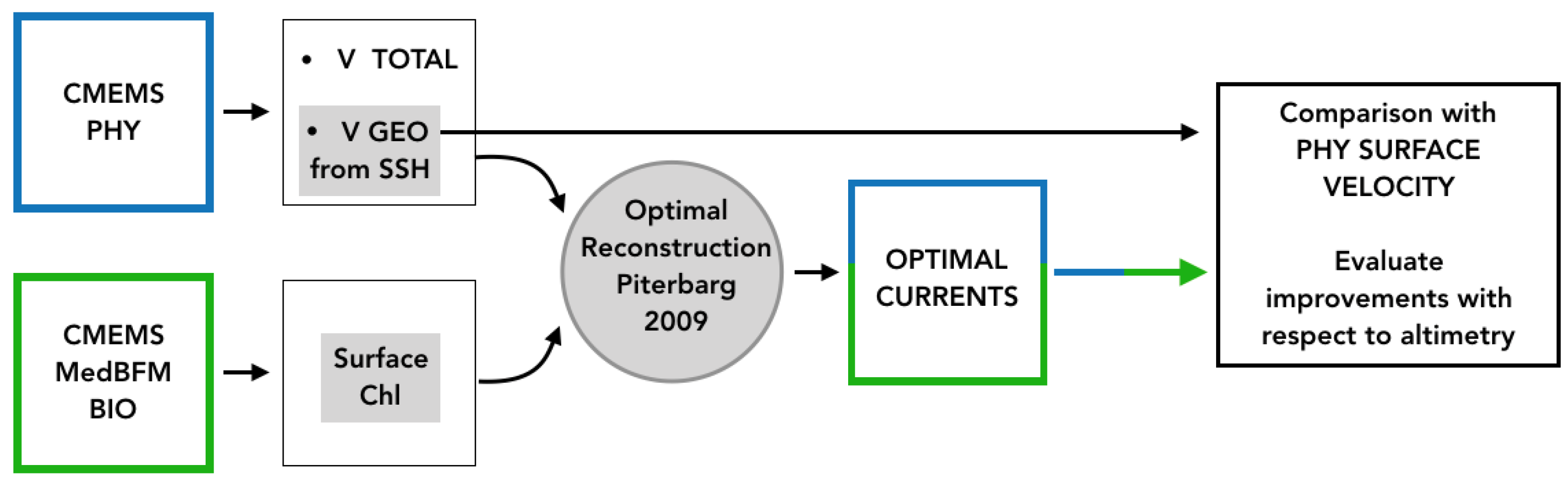
  • The CMEMS Mediterranean Sea Physics Analysis and Forecast (PHY) Model
    The Mediterranean Forecasting System is a hydrodynamic primitive equations model for the Mediterranean Basin and the Atlantic Ocean off Gibraltar-Straight [39]. It is available via the CMEMS web portal (CMEMS Product ID: MEDSEA-ANALYSIS-FORECAST-PHY-006-013). The model provides daily and hourly fields of horizontal currents, 3D temperature, salinity and free-surface elevation for the Mediterranean Area as well as a small region of the Atlantic Ocean in proximity of the Gibraltar Strait. We collected the daily outputs within the boundaries of the Mediterranean Basin (30 to 46 N and −6 to 37 E), which are provided on a 1/24 regular grid and 125 unequally spaced vertical levels. The core of the hydrodynamical model is the Nucleus for European Modelling of the Ocean (NEMO, version v3.6), and the wave component is provided by Wave Watch-III. The numerical simulations take advantage of data-assimilation of temperature and salinity vertical profiles as well as along-track sea-level anomaly observations.
  • CMEMS Mediterranean Biogeochemical Flux, MedBFM (BIO) Model
    MedBFM BIO is a biogeochemical model for the Mediterranean Sea distributed via CMEMS [CMEMS Product ID MEDSEA-ANALYSIS-FORECAST-BIO-006-014] [40,41,42]. This model provides daily 3D outputs of ocean biogeochemical variables (Chl, nutrients, oxygen, etc.) on the same horizontal and vertical grids as the PHY model (1/24 regular horizontal grid and 125 vertical levels), which also provides the physical forcing that contributes to the biogeochemical systems evolution. MedBFM BIO also includes assimilation of satellite-derived surface Chl concentration, oxygen, nitrates and phosphates’ vertical profiles.
  • The Synthetic Altimeter-Derived Currents
    The Synthetic Altimeter-derived Currents (SAC) are simulated using SSH data from the CMEMS PHY model. First, the Sea Level Anomaly (SLA) information is obtained from the model outputs using the following formula:
    SLA = SSH ( MDT 0.344 )
    with the Mean Dynamic Topography (MDT) provided by the CMEMS product. The 0.344 constant (given in m) allows to center the SLA values on the Mediterranean region during 2017, so that the spatio-temporal mean of SLA equals zero. The obtained simulated SLA exhibits rapid sea level changes across the whole basin occurring over 2–3 days. Indeed, recent progress in ocean modelling now allow for simulating rapidly moving atmospheric pressure disturbances causing storm surges and inverse barometer effects. This raw SLA cannot be handled by the mapping method based on Optimal Interpolation. With real altimetry data, this large-scale high-frequency variability is removed using the Dynamic Atmospheric Correction (DAC) derived from atmospheric forcing [43]. However, the application of this correction to our simulation is not satisfactory as some residual effects are still noticeable. The alternative consists of filtering out the large-scale patterns to focus on the reconstruction of the small-scales and therefore local gradients. A Loess filter with a cut-off frequency of 600 km is applied to SLA maps in order to preserve small-scale features, such as eddies. The small-scale SLA is finally sampled along the actual tracks of Jason-3, Sentinel-3A, SARAL/Altika, and Cryosat-2 missions, using the SWOT simulator software [44]. Measurement errors and noise representative of each mission are added to the SLA value to simulate the altimeter data (see Table 1 or Quality Information Document for CMEMS product ID SEALEVEL-GLO-PHY-L3-NRT-OBSERVATIONS-008-044). This 4-satellite constellation is representative of the CMEMS near-real-time constellation during 2017.
    These along-track synthetic measurements are then used in input of DUACS (Data Unification and Altimeter Combination System) to produce gap-free SLA maps. Based on optimal interpolation (OI), the mapping of SLA follows the DUACS DT2018 configuration for the Mediterranean Sea, described in [20]. In particular, the correlation spatial scales range from 75 to 200 km, depending on the location, while temporal scales are set to a constant value of 10 days. It means that, for a given space–time grid point, only along-track observations that lie within 75 to 200 km and 10 days with respect to the grid point are selected. The modelled large-scale SLA patterns (filtered out before the mapping) and the reconstructed small-scale maps are finally recombined in order to compute the daily surface currents via the geostrophic approximation. Such data are provided on a regular 1/8 grid, as for the present-day version of the CMEMS Altimeter-derived gridded regional products for the Mediterranean Sea.
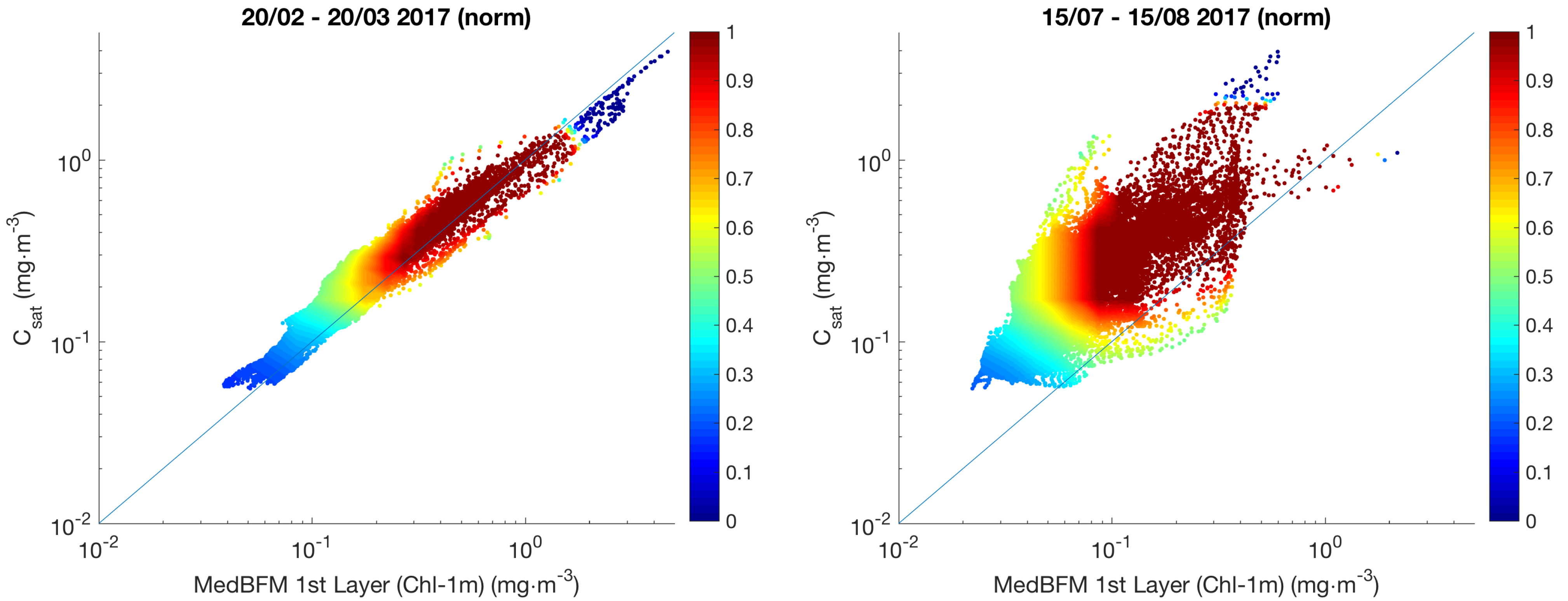
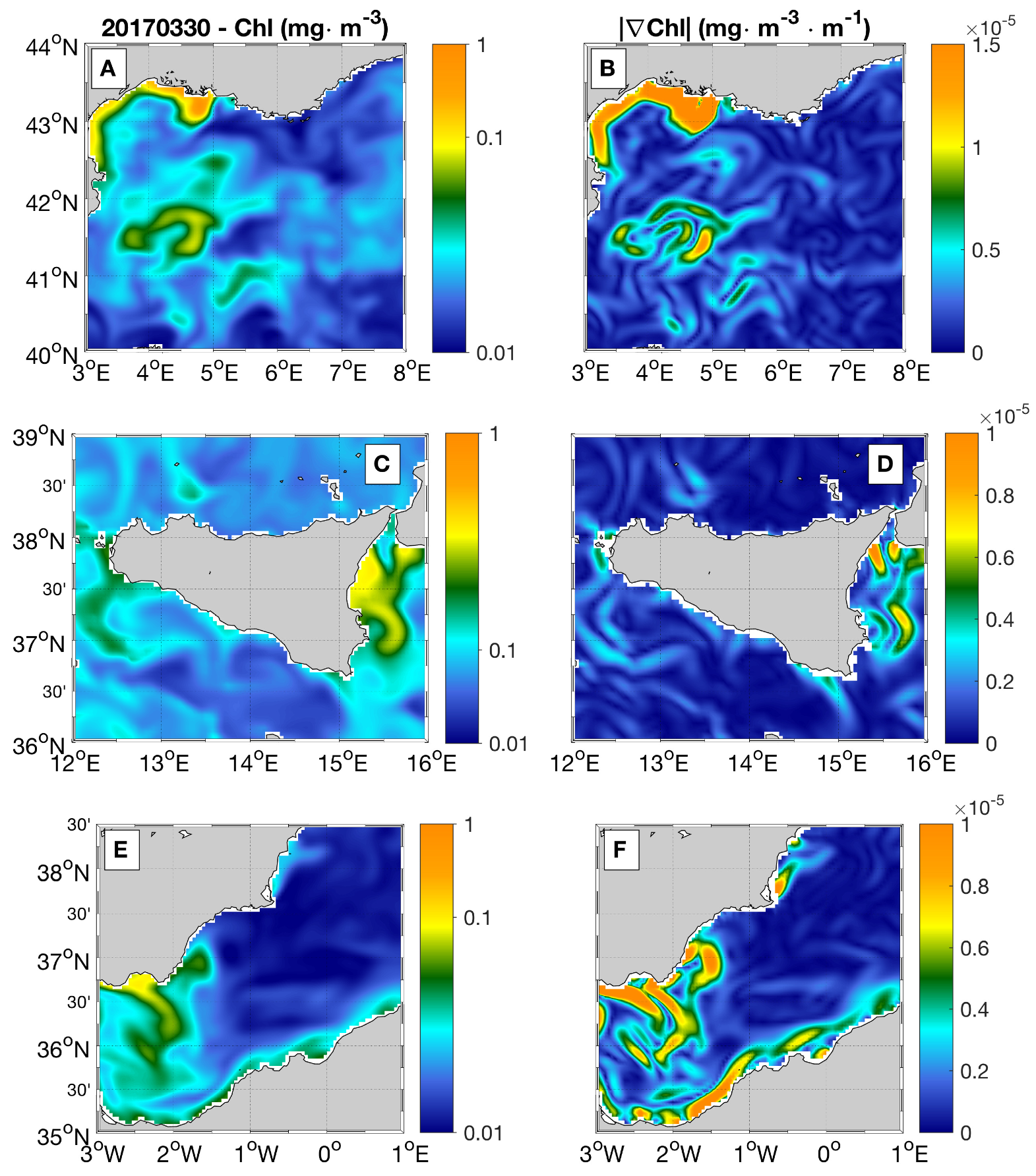
  • The Synthetic Satellite-Derived Chl
    Space-based bio-optical oceanic variables such as the surface Chl concentration are derived from passive observations by sensors mounted on board polar satellites through algorithms calibrated with in situ observations. The Chl remote sensing principle is based on measurements of the visible radiation that, after penetrating the first meters of the surface oceanic layer, is scattered back towards the atmosphere in the direction of a satellite sensor. Therefore, the satellite-derived Chl is an integrated quantity over the first meters of the oceanic water column.
    Since our study constitutes a testbed for applying the optimal reconstruction to satellite-derived data, we evaluated a satellite-derived equivalent surface Chl “C sat ” from the CMEMS BIO model for the entire year 2017. We relied on the “C sat ” expression provided by Morel and Berthon 1989 [45]:
    C sat = 0 z p C ( z ) e 2 kz dz 0 z p e 2 kz dz
    where “C” is the marine Chl value at the depth “z”, “k” is the light attenuation coefficient, and “Z p ” is the light penetration depth along the water column. In our study, the quantities appearing in (2) were computed from the CMEMS BIO model and Z p ranged from 5 to 30 m, depending on the location and season. Using C sat is more rigorous than approximating the satellite equivalent Chl via the first layer output of the MedBFM model (≃1 m depth). A comparison between the Chl-1m and the C sat is carried out in two distinct periods of 2017: the high biological production (20 February to 20 March 2017) and the low biological production periods (15 July to 15 August 2017) also accounting for past studies on the Mediterranean Sea trophic regimes [37]. The normalized scatter density plots of the C sat and Chl-1m are obtained computing the time-averaged Chl maps in the two aforementioned periods for the entire Mediterranean basin. The results proved that the Chl-1m mostly underestimates the C sat (Figure 1). This is more evident during the low production period, when the Z p values appearing in (2) are larger due to a decreased near surface water turbidity and the larger Chl concentrations (the Deep Chl Maximum) are found at larger depths [46], increasing the discrepancies between Chl-1m and C sat .

2.2. The Work Logic

The work logic of our OSSE is sketched in Figure 2.
The CMEMS PHY and BIO models are used to generate synthetic altimeter-derived geostrophic currents and satellite-derived Chl concentrations in the Mediterranean Sea, as detailed in Section 2.1. Then, the optimally reconstructed currents (OPtimal Currents, OPC hereinafter) are computed according to the PIT09 equations (provided in Section 2.3) for the entire year 2017 and compared to the PHY model surface layer outputs (our ground-truth current field). In this way, a direct comparison of the 2D Eulerian currents can be carried out, enabling to have equally significant statistics for every grid point of our study area.

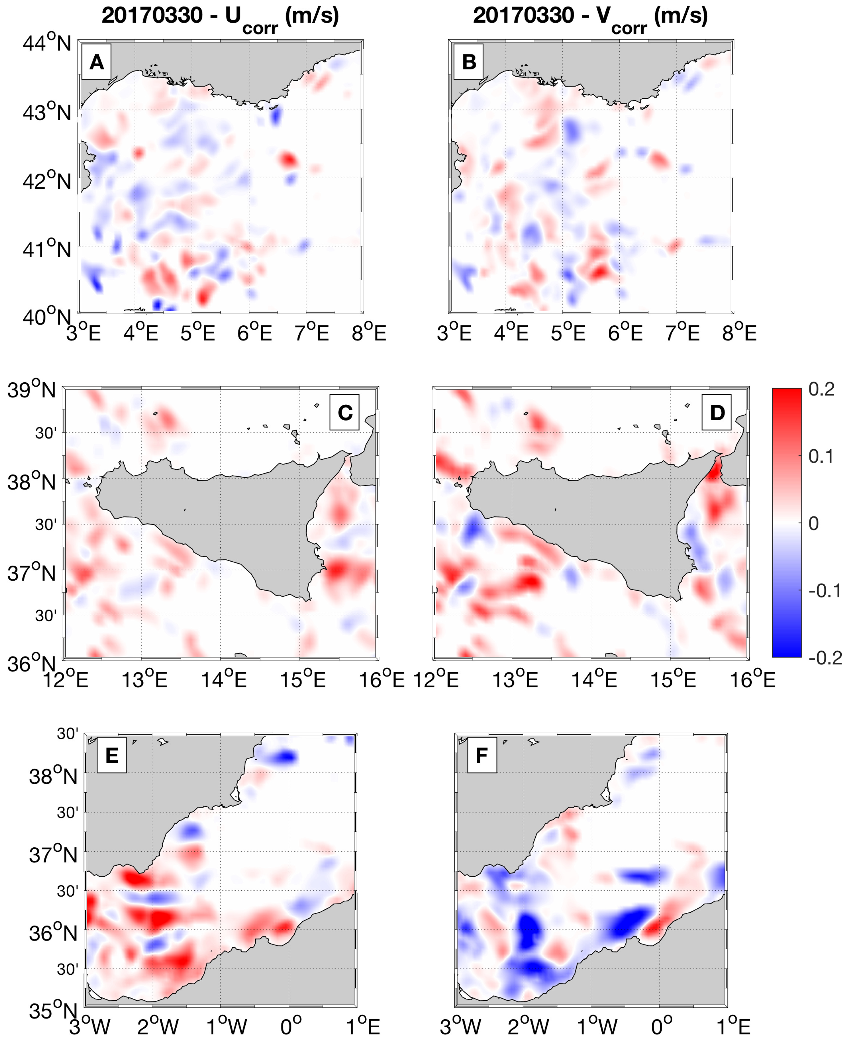
2.3. Methods: Rationale of the Optimal Reconstruction

The ocean surface currents are computed from synthetic altimetry measurements combined with higher resolution synthetic satellite Chl observations, relying on the algorithm firstly developed by Piterbarg [26] and Rio et al. [27]. The principle is to constrain the surface geostrophic flow to follow the evolution of a surface tracer, assuming the tracer can be derived independently and that it is characterized by higher spatial-temporal resolutions than the geostrophic flow, like in our study. With this approach, we attempt to extract useful dynamical information from the surface oceanic tracer evolution to enhance the spatial-temporal content of the geostrophic currents. For clarity, the derivation of the optimal currents is reminded in this section. The sea surface currents are inferred from (3):
Chl t + u Chl x + v Chl y = F
In (3):
  • (x,y) are the zonal and the meridional directions;
  • ( u , v ) are respectively the zonal and meridional components of the ocean surface flow;
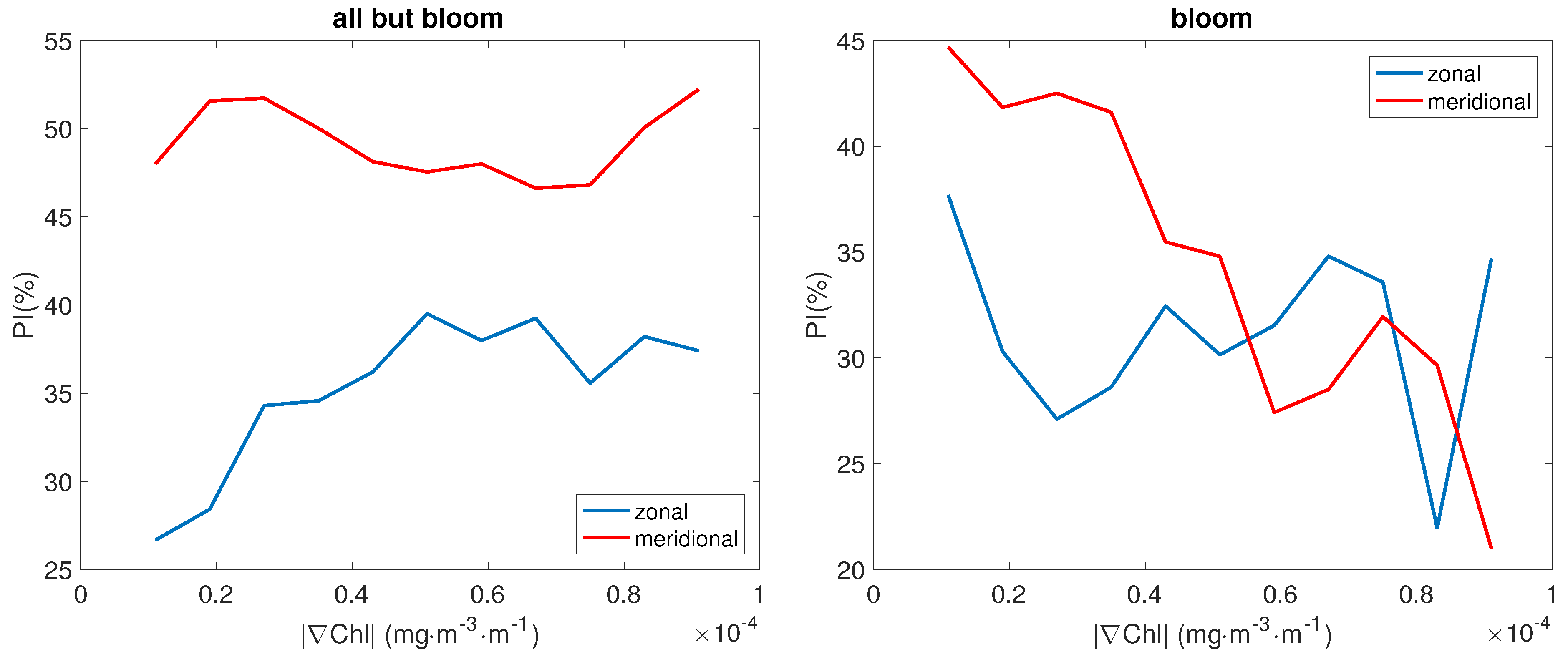
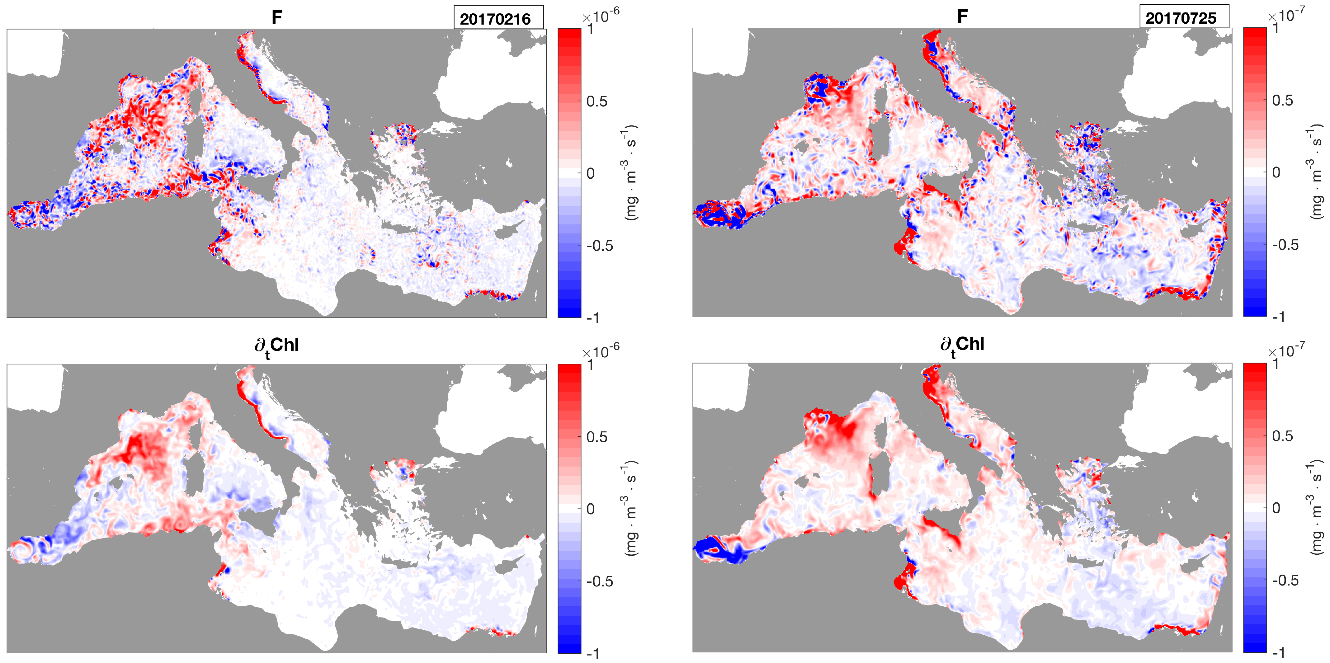
  • F is the forcing term, representing the Chl source and sinks which, in the present case, include both biological and environmental factors. In particular, F includes contributions from the marine currents’ vertical advection, horizontal and vertical diffusion as well as the biogeochemical reactions involved in the phytoplankton dynamics [47]. The contributors to the source/sink terms can have different relative magnitudes according to space and time. For example, we expect vertical advection to be dominant under high wind stress conditions that may trigger upwelling currents or in the presence of mesoscale/submesoscale features generating strong vertical motions [48,49]. In addition, biogeochemical reactions become dominant during the so-called “Chl-blooming periods”, i.e., when the near-surface Chl production increases due to an abundance of light and nutrients (e.g., inorganic carbon dioxide, silica, nitrates and phosphorus) involved in the phytoplankton photosynthetic activity [37,38].
PIT09 [26] derived the expressions of an optimized flow field accounting for the merged contribution of a large-scale, background flow with the dynamical information contained in high-resolution tracers. If the background flow is given by the Synthetic Altimeter Currents (SAC) and the high-resolution tracer by Chl, the zonal and meridional OPtimal Currents (OPC) can be expressed by (4):
u OPC = u SAC A ( Au SAC + Bv SAC + E ) A 2 + B 2 = u SAC + u CORR v OPC = v SAC B ( Au SAC + Bv SAC + E ) A 2 + B 2 = v SAC + v CORR
where A = x Chl , B = y Chl , E = t Chl F . In (4), the subscript “t” stands for temporal derivative and the subscripts “x,y” respectively indicate the spatial derivative in the zonal and meridional directions.
Equation (4) expresses the PIT09 method rationale: the geostrophic currents are corrected by means of a factor ( u CORR , v CORR ) depending on the spatio-temporal derivatives of the high-resolution tracer observations and on the forcing term (F) regulating the tracer dynamical evolution.
Equation (4) is valid when the forcing term F is known perfectly, like in the present study where F is derived from Equation (3). In case the F term cannot be derived perfectly, the set of Equations (4) is modified accordingly and also requires estimating and calibrating the uncertainties on F and on the ( u , v ) SAC , as extensively illustrated by [26,28,29,31].

2.4. Methods: Optimal Reconstruction Quality Assessment

Using the daily data detailed previously and accounting for Equations (3) and (4), we computed one year (2017) of optimal currents. The performances of the optimal reconstruction were evaluated by means of qualitative and quantitative assessments, respectively via visual inspection and by computing the Root Mean Square Differences (RMSD, Equation (6)), Percentage of improvement (PI, Equation (5)), temporal standard deviation (STD, Equation (7)) and spatial spectral properties of the altimeter-derived, optimal currents and CMEMS PHY modelled surface currents (our validation benchmark):
PI U , V = 100 1 RMSD U , V OPC RMSD U , V SAC 2
RMSD U , V SAC / OPC = i = 1 N [ ( U i , V i ) SAC / OPC ( U i , V i ) PHY ] 2 N
STD U , V SAC / OPC / PHY = i = 1 N [ ( U i , V i ) SAC / OPC / PHY ( U i , V i ) SAC / OPC / PHY t ] 2 N
In (5)–(7):
  • the superscripts SAC, OPC, PHY, respectively, stand for synthetic altimeter currents, optimal currents, and CMEMS PHY modelled surface currents;
  • U,V respectively indicate the zonal and meridional flow;
  • the i index goes from 1 to N = 365, i.e., the number of the daily surface currents data during 2017;
  • the t operator in (7) indicates a time average over the year 2017;
Briefly, Equation (5), based on inputs provided by (6), quantifies the ability of the optimal reconstruction to reproduce the CMEMS PHY currents compared to the altimeter estimates. This is achieved computing a percentage of improvement (PI) for every grid point of our simulation area. On the other hand, Equation (7) is used to quantify the enhancement of the optimal currents temporal variability compared to the altimeter system. Indeed, the STD is computed with respect to the 2017 time averaged surface currents: higher STDs will correspond to higher temporal variability of the signal under evaluation.
Finally, a spatial spectral analysis is also performed. From the Kinetic Energy (KE) fields of the SAC, OPC and CMEMS PHY modelled surface currents, we compute the KE power spectral density (PSD) in two land free areas of the Mediterranean Sea (in the Levantine Basin and in proximity of the Algerian Current). The PSDs are obtained via spatial Fast-Fourier-Transform analysis using the same technique proposed by [9,50]. Longitudinal KE samples are extracted from the KE fields; then, the corresponding PSD are computed for every latitude and time. The PSDs are finally averaged to obtain a single spectrum for each dataset under evaluation. With this approach, we determine the amount of KE spatial variance found at different scales in the three surface currents’ datasets, allowing for estimating and intercomparing their effective spatial resolution.

3. Results

Here, we illustrate the qualitative and quantitative assessments of the optimal currents, based on the validation metrics described in Section 2.4.

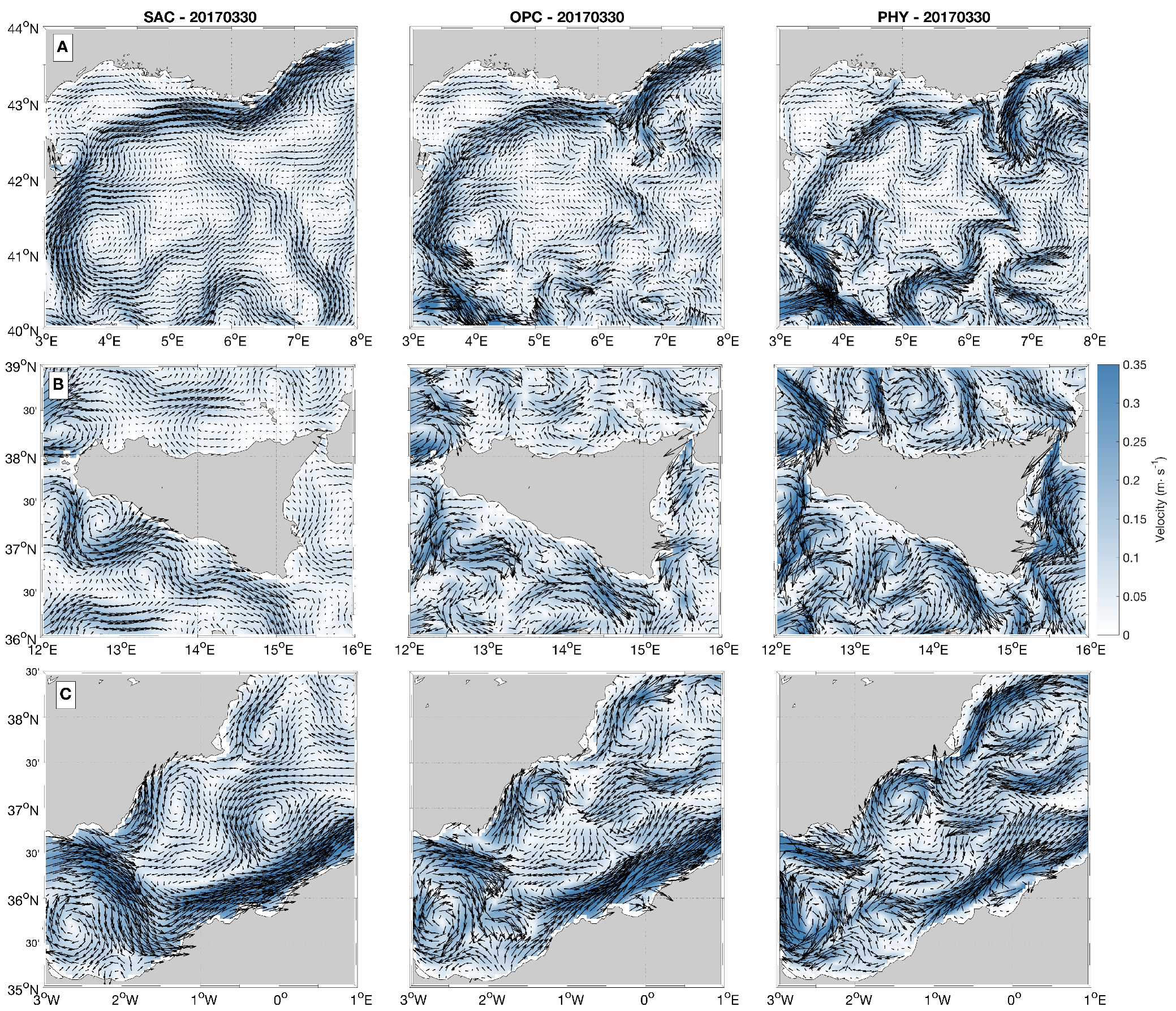
3.1. Qualitative Assessment

The optimally reconstructed currents are presented in three test cases on 30 March 2017, sketched in Figure 3. In our numerical study, the late-March time window is a favourable one for the OPC reconstruction. In this period, higher sea surface Chl concentrations result from the blooming activity [37,38], facilitating the extraction of dynamical information from the surface Chl patterns. We chose three well-known dynamically active areas of the Mediterranean Sea [36]: the Northwestern Mediterranean in correspondence with the Liguro-Provencal Current, the area in proximity of the Alboran Sea and the Sicily Channel; the last region was also investigated by past studies based on a similar approach [29,30]. Figure 3A–C allow for inspecting simultaneously the surface circulation field described by the SAC and OPC datasets, with the CMEMS PHY model providing the ground truth. In general, the SAC underestimates the maximum current intensities, providing a smoother description of the main meanders, filaments, and eddy-like features. Some examples of the circulation features not correctly captured by the SAC dataset in the three analysed areas are provided below,
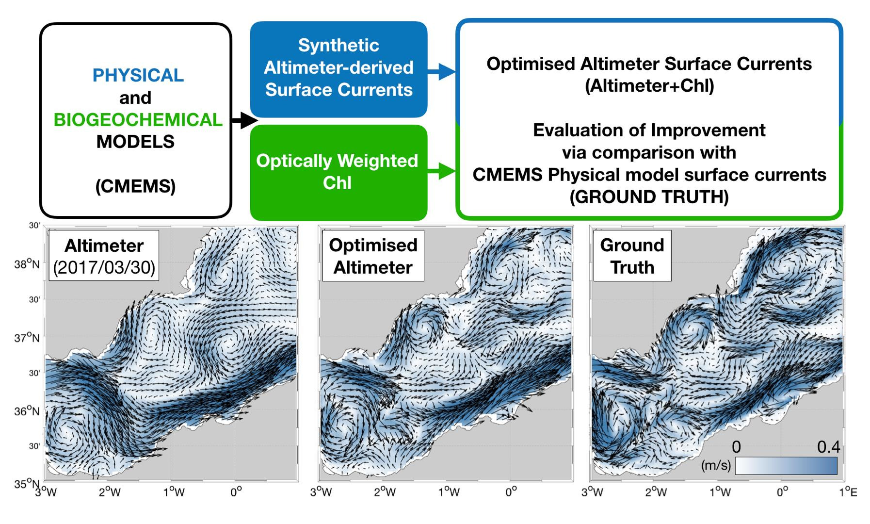
  • Figure 3A: the anticyclonic meander found at 43 N–7 E, the two eddy system located at 41.3 N–4 E and the meandering tongue flowing from 40 N–5 E towards the northeastern section of area A;
  • Figure 3B: the current system flowing off the western tip of Sicily, perpendicular to the coastline (at the approximate location of 37.5 N–12.5 E), the eddy located at 38.5 N–12 E and the western boundary of the the Messina Rise Vortex (37 N–15.5 E);
  • Figure 3C: the Alboran gyre and multiple eddies system found north of the 36.5 N parallel, particularly the one circulating at 37 N–1.5 W.
The aforementioned features are almost fully recovered by the OPC datasets (Figure 3). Recalling the basics of Equation (4), the improvements must come from the surface tracer gradients field: they enable to build the correction terms for the SAC dataset and carry out the optimal reconstruction. An additional qualitative analysis, depicted by Figure 4 and Figure 5, indicates the validity of this assumption. The figures show the patterns of the surface Chl spatial gradient magnitude, | Chl | = ( x Chl ) 2 + ( y Chl ) 2 , and the corrections factors (u corr , v corr ) computed with (4). Comparing Figure 3, Figure 4 and Figure 5 allows for confirming that the main corrections are found in areas where the | Chl | is larger than ≃2·10 6 mg·m 4 and exhibits patterns related to the advection of the horizontal currents. Elsewhere, the optimal reconstruction cannot extract dynamical information from the surface tracer patterns. We also notice that the case ( x C h l ) 2 + ( y C h l ) 2 = 0 , following Equation (4), is not accepted for the optimal reconstruction. In our numerical study, this condition only happened in 0.1% of the analysed cases and mostly during summertime (late June to early July), i.e., when the biological productivity is damped compared to the late-winter/early-spring months [37]. If we exclude the coastal areas, the summertime surface Chl fields are mostly O ( 10 2 ) mg·m 3 against the O ( 1 ) mg·m 3 found during winter. Moreover, the summertime Chl surface fields tend to be more uniform throughout the basin, hindering the appearance of surface Chl gradients related to the horizontal currents advection.

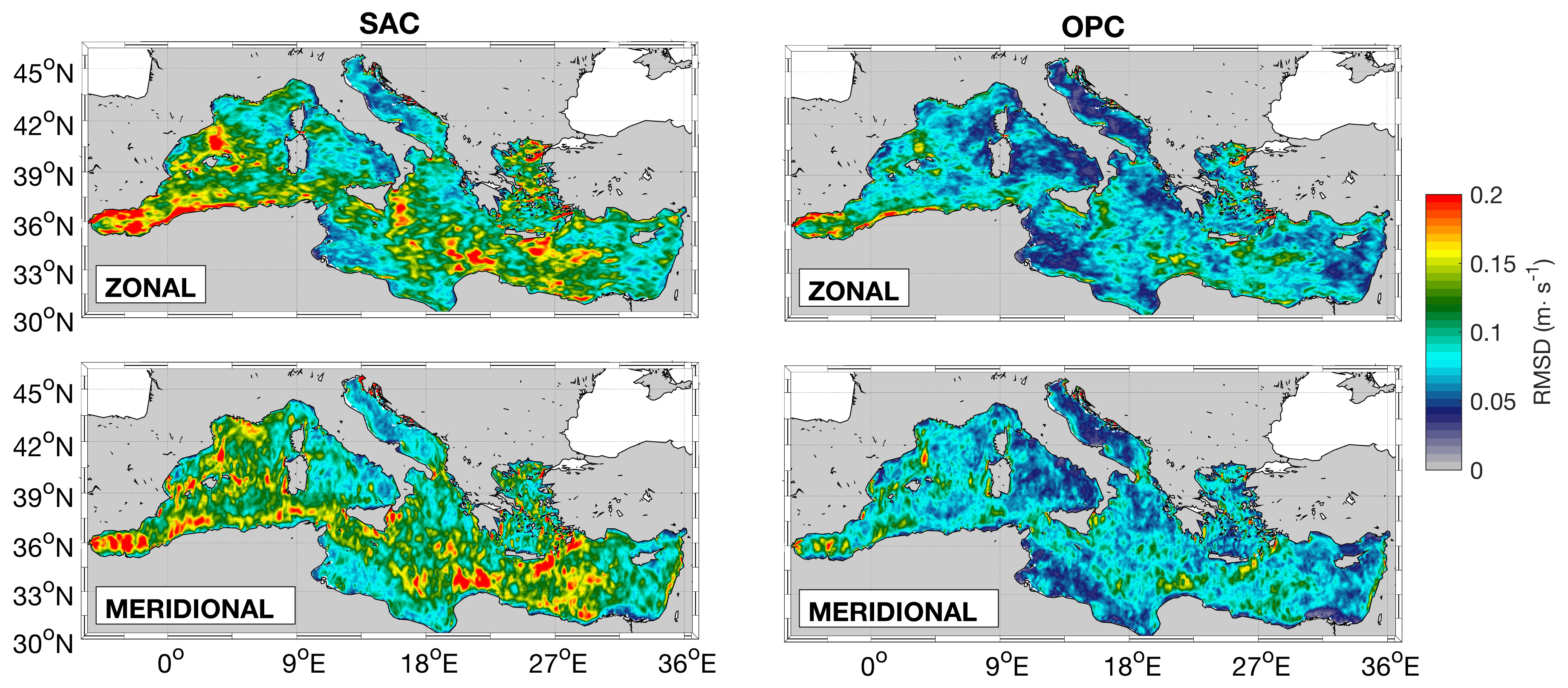
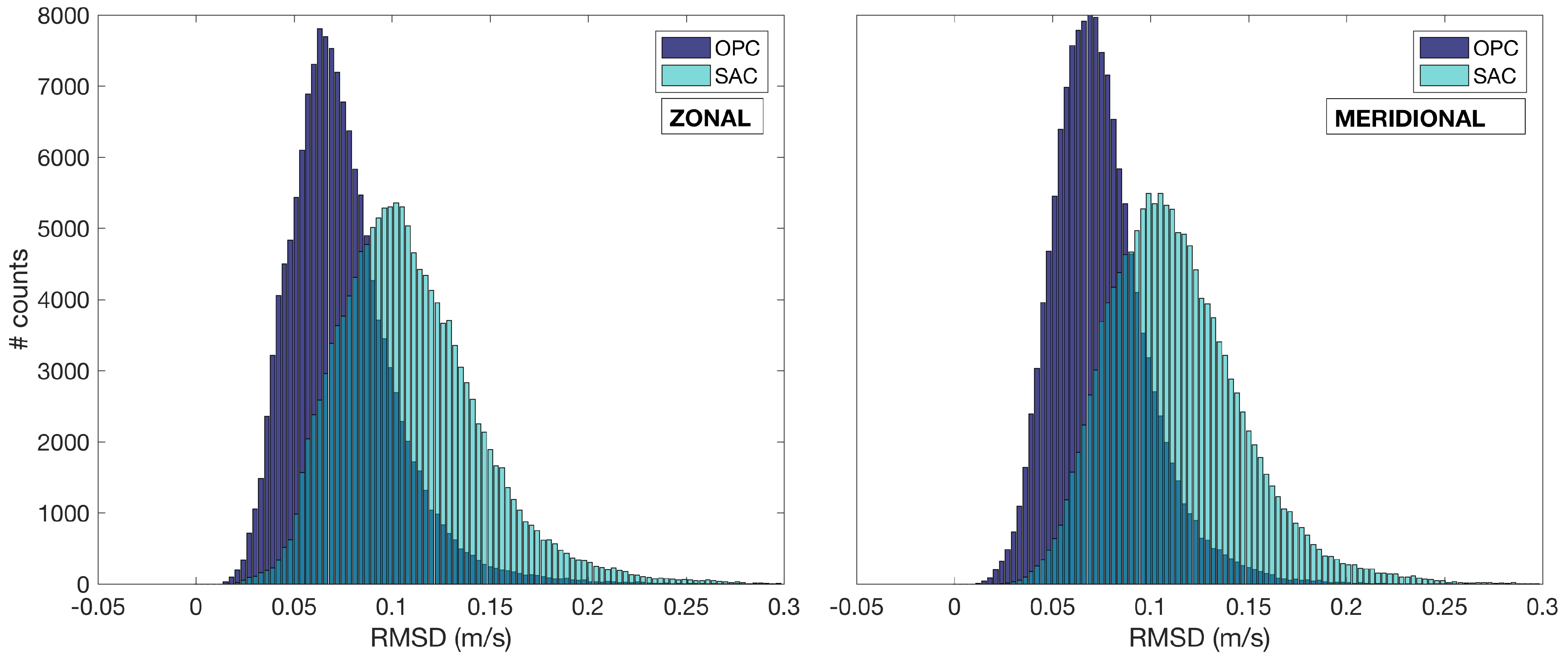
3.2. Quantitative Assessment

Following Equation (6), we present some quantitative performances of the optimal reconstruction, sketched in Figure 6. Based on the 2017 daily data, we compute the RMSD of the Synthetic Altimeter (SAC) and OPtimal Currents (OPC), using the CMEMS PHY surface outputs as a validation benchmark. This operation is repeated for both the zonal and meridional surface flows. When the SAC are analysed, we find RMSDs always equal to or larger than 5 cm·s 1 , with maximum values reaching 30 cm·s 1 in the Western Mediterranean, in the Atlantic Ionian Stream across the Sicily Channel and in many areas of the Levantine Basin (roughly from 18 to 30 E), including the area south of Ierapetra.
When the information from the surface Chl is introduced within the Altimeter currents, large improvements are observed at the basin-scale. Patches of RMSD ≃20 cm·s 1 only cover 2 to 3% of the basin and are mostly limited to coastal areas in the Western Alboran sea. Overall, the RMSD of the OPC is mostly around 7 to 8 cm·s 1 for both components of the motion, against the ≃13 cm·s 1 found in the SAC case. This is clearly summarised by the distributions of RMSD values reported in Figure 7: the improvements of the OPC with respect to the altimeter currents result in narrower OPC RMSD distributions, with a significantly larger number of cases shifted left towards the zero value.
The RMSD values enable building additional indexes that quantify the skill of the optimal reconstruction, e.g., through the percentage of improvement, PI, described by Equation (5). This analysis was performed accounting for the entire time series of the SAC and OPC datasets (i.e., relying on more than 5 · 10 7 data for both datasets) considering observations lying in | C h l | areas ranging from 10 5 to 10 4 mg·m 3 ·m 1 for both the zonal and the meridional currents. Figure 8 shows that the zonal and meridional OPC improve the altimeter estimates by about 20 to 50% and that the PI is generally larger for the meridional component of the motion. This is easily explained considering the north–south orientation of the nadir-looking altimeter ground tracks, allowing for deriving more accurate zonal surface currents via the geostrophic approximation [28,31,51]. More in detail, the overall behaviour of the PI is summarised by the left panel of Figure 8, which considers all the 2017 data except for the mid-February to mid-March period (far from the main Chl blooming events, [36,37]). The meridional PI is fairly constant, exhibiting values oscillating between 45% and 52%, while the zonal PI increases from 27% to 38% when the local Chl spatial gradients are intensified. As a result, the PIT09 method reproduces higher quality optimal currents for increasing local | C h l |, in a good agreement with past studies based on the use of SST data [28,29,31]. On the other hand, Figure 8-right shows that the PIs tend to decrease towards highest | C h l | areas between mid-February to mid-March 2017 (i.e., during the main Chl blooming events found in the MedBFM simulations). Though the zonal and meridional PIs are still positive, the result suggests that, during the blooming events, the highest | C h l | may not fully optimise the altimeter derived horizontal currents, as Chl evolution is strongly dominated by biological and environmental factors favouring significant phytoplankton growth and complex interactions within the trophic network.
The benefits of the optimal reconstruction are also given by enhancements of the spatial and temporal variability of the OPC dataset compared to the SAC. Such benefits are quantified by means of Equation (7) and via the spatial spectral analysis illustrated in Section 2.4. To investigate the SAC and OPC temporal variabilities, we first derive the 2017 time-averaged surface currents (zonal and meridional) for the SAC, OPC, and PHY datasets. Then, we compute the SAC, OPC, and PHY currents’ temporal standard deviations (STDs) using the 2017 daily data. The results are reported in Figure 9. The CMEMS PHY data show STDs around 10 to 25 cm·s 1 throughout the Mediterranean, with only a few areas characterised by 5 cm·s 1 values for both the zonal and the meridional flow. An ideal optimal reconstruction should reproduce the same PHY STD values. This is not the case for the two components of the optimal currents, which exhibit STD values mostly centered around 7 cm·s 1 and reaching 20 cm·s 1 in a few areas of the western Mediterranean. However, an interesting result is shown in the bottom panels of Figure 9, showing maps of zonal and meridional STD differences ( Δ STD) between the optimal and synthetic altimeter currents. The Δ STDs are larger than zero in 80% of the Mediterranean Sea, confirming that the optimal currents are characterised by an enhanced temporal variability compared to the Altimeter estimates. We repeated this analysis on timescales of 10 days, which is the temporal search radius used in the SAC optimaI interpolation scheme (as for the DUACS system, discussed in Section 2) and can be thought of as our lower limit for the SACs’ effective temporal resolution. In this case, we also obtained Δ STDs > 0 in more than 80% of our study area, suggesting that the OPC has larger effective temporal variability than the synthetic altimeter estimates, as shown by Figure 10.
The optimal currents effective spatial resolution is also quantified using the 2017 daily data involved in our study. After computing daily maps of surface Kinetic Energy (KE), we derive the KE power spectral density (PSD) in two land-free areas of the Mediterranean Sea: the “WEST” and “EAST” areas, with respective horizontal extents from 37.5–38.5 N/0–11 E and 33–34 N/16–34 E, depicted in Figure 11. As discussed in Section 2, the PSDs are obtained from spatial Fast Fourier Transform analysis and enable checking simultaneously the properties of the SAC, OPC and CMEMS PHY currents (Figure 11). The OPC (blue) and the SAC (red) spectra behave similarly in the WEST and EAST areas. For low wavenumbers (scales up to 100 km), the spectra are fully superimposed, indicating that the two fields are describing the same surface dynamics. Going towards smaller spatial scales, the two spectra begin to separate, the OPC one always exhibiting larger values, closer to the theoretical predictions on surface 2D turbulence (K 5 / 3 slope, with K the wavenumber, [51]). As a result, the optimal reconstruction is describing more accurately the finer circulation structures compared to the SAC. The CMEMS PHY ground truth KE spectra (light blue) are also reported and indicate good agreement with the optimal currents, further confirming the potential of the PIT09 method for improving the effective spatial resolution of the surface currents. Based on our analyses, the PSD of the optimal currents fully recovers the ground truth spectral properties until scales of ≃30 km.

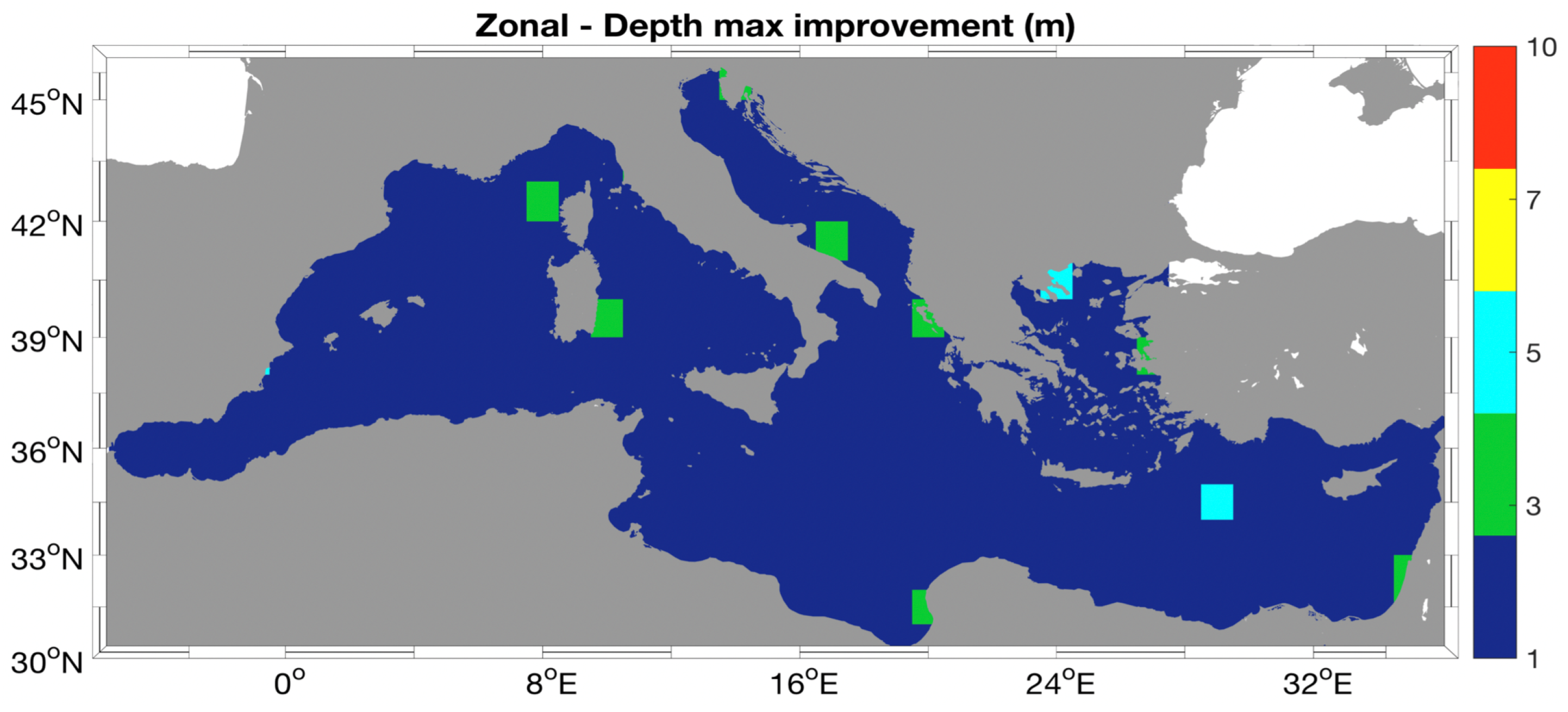
3.3. Effective Depth of the Optimal Currents

As discussed in Section 2, the PIT09 method has been implemented relying on an optically weighted Chl dataset. This is obtained via Equation (2) integrating contributions from several layers of the water column, i.e., from the sea-surface to the light penetration depth Z p [45]. Maximum penetration depths can reach 30 m in the Mediterranean area; therefore, we evaluate whether a vertically integrated “near surface” oceanic tracer can impact the effective depth of the optimally reconstructed currents. To this scope, we compare the PI of the optimal currents (Equation (5)) using several modelled PHY currents as ground truth, selecting outputs at 1, 3, 5, 7, and 10 m depth. In Figure 12, the PI is presented for both the zonal and meridional flows (blue and red lines, respectively). The figure suggests that the OPC is closer to the PHY surface layer currents, i.e., the 1 m depth output. In that case, we obtain the highest basin-scale averaged PI, around 45%, while, for larger depths, the PI decreases monotonically, reaching ≃20% at 10 m depth (eventually becoming negative for larger depths, not shown). The monotonic decrease of the PI, following Equations (5) and (6), indicates that for larger depths, the OPC RMSD increases due to the OPC deviation from the PHY modelled currents.
The effective depth of the OPC is also evaluated as a function of space. This is achieved computing the OPC improvements with respect to the 1, 3, 5, 7, 10 m PHY currents in 1 × 1 boxes. The results are reported in Figure 13 only for the zonal OPC (the behaviour of the meridional currents is analogous). In the figure, the colours stand for the depth at which we record the maximum PI of the OPC, evaluated via Equation (5) and based on one year statistics (2017). More than 90% of the basin exhibits maximum PIs when the surface layer (1 m) PHY currents are considered as a benchmark. Very rarely, and mostly in coastal zones, some PIs are larger at 3 or 5 m depths. Nevertheless, in these cases, the PI differences between the surface and the deeper layers never exceed 0.4%. We concluded that our optimal reconstruction mainly yields information on the sea-surface circulation.

4. Discussion and Conclusions

The OSSE has showed encouraging results to improve the altimeter-derived surface currents in the Mediterranean Area by exploiting the combination of SSH-derived and surface Chl data with the PIT09 method. This study relied on numerical hydrodynamical and biogeochemical models distributed within the Copernicus Marine Service CMEMS, providing gap-free data that can be manipulated to simulate satellite-derived observations and, at the same time, to rely on gap-free fields that can be used as a validation benchmark. Specifically, the CMEMS PHY hydrodynamical model has been used to simulate the altimeter-derived currents and to extract total surface currents, e.g., our ground truth. The CMEMS MedBFM model was used to simulate the satellite surface Chl fields.
In the simulated scenario, the PIT09 method allowed for computing a one year long time series of optimal currents by merging the altimeter-derived currents (1/8 horizontal resolution) with the surface Chl data (1/24 horizontal resolution). Analysing the optimally reconstructed surface currents, we could mainly determine that:
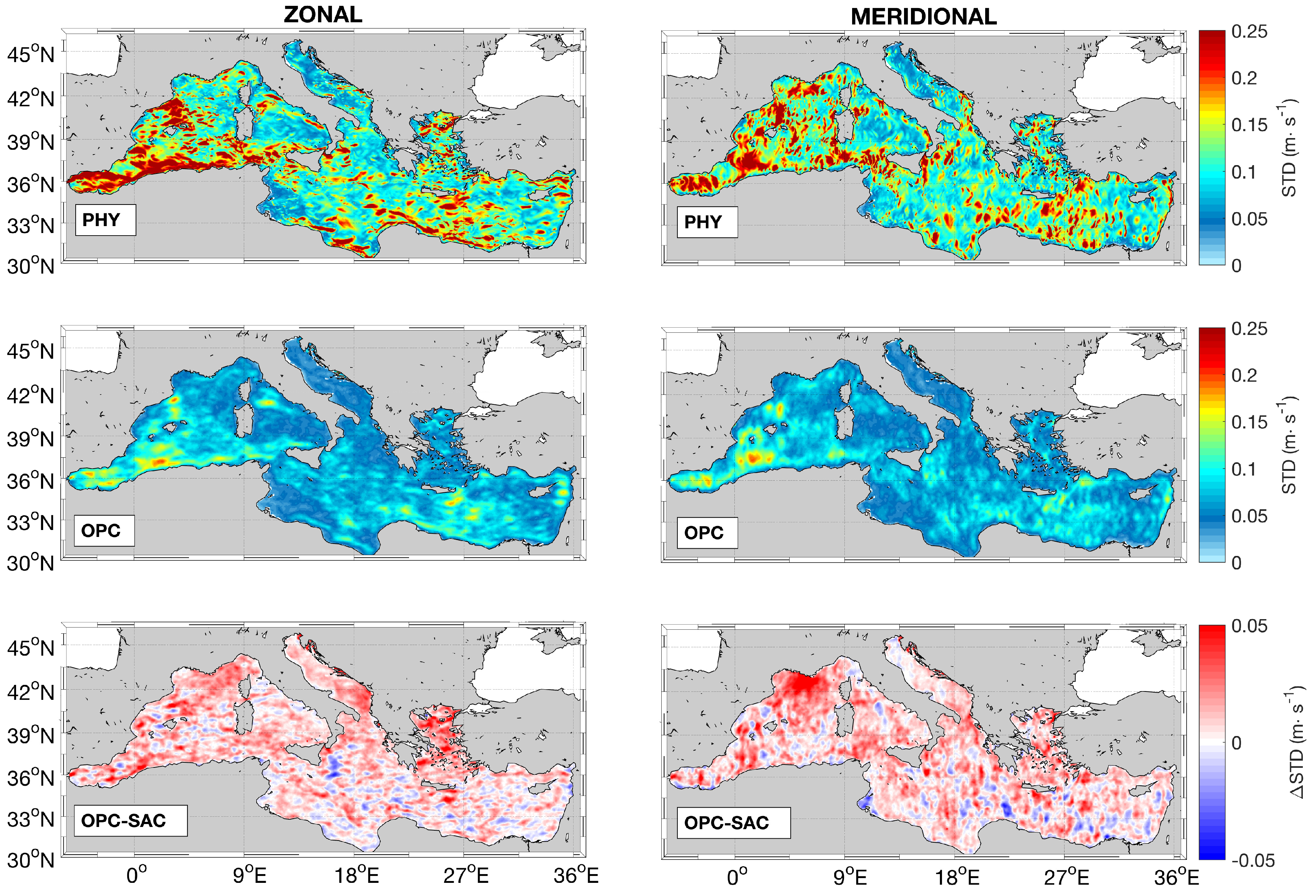
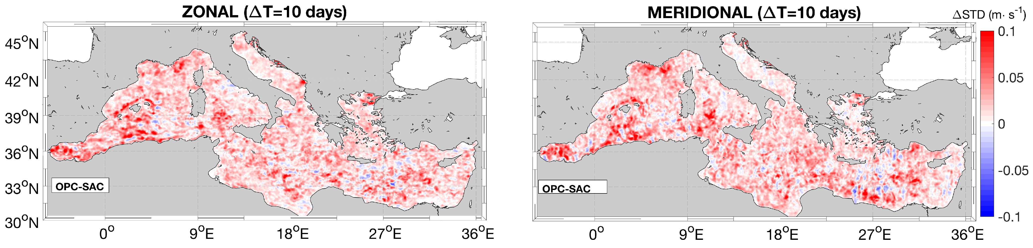
  • the effective temporal resolution of the optimal currents is enhanced compared to the altimeter estimates. This was obtained computing the temporal standard deviations (STD) of the Synthetic Altimeter-derived and OPtimal surface Currents (SAC and OPC, respectively). The difference between the OPC and SAC STDs, computed on both annual and weekly timescales, is positive in 80% of the Mediterranean, demonstrating an enhanced temporal variability;
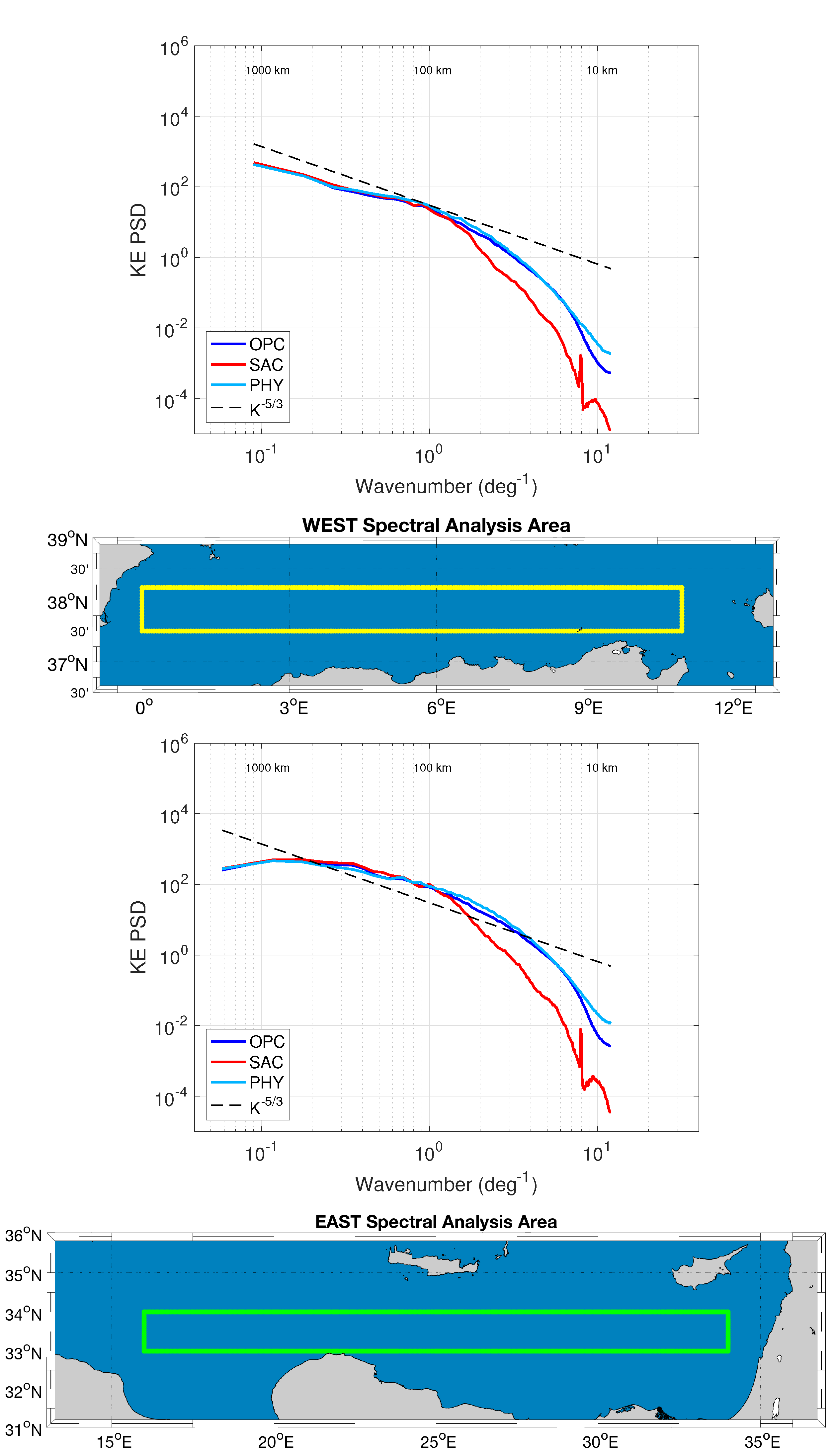
  • the spectral analyses of the SAC, OPC and CMEMS PHY Kinetic Energy fields suggest that the OPC fully recovers the surface dynamics until scales of 30 km that we defined as the OPC effective spatial resolution. Following the same spectral analysis, the SAC dataset fully describes larger mesoscale features around 100 km;
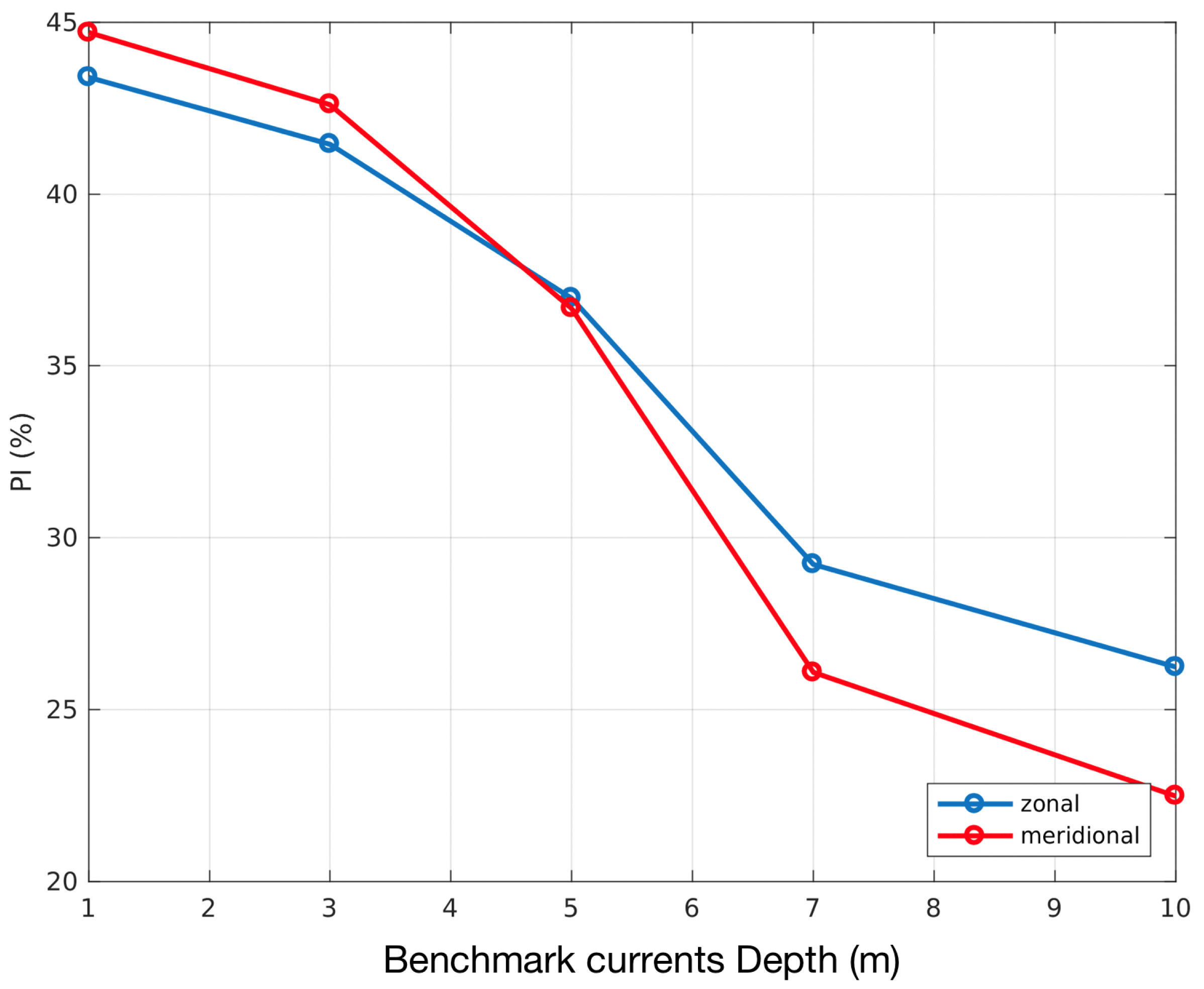
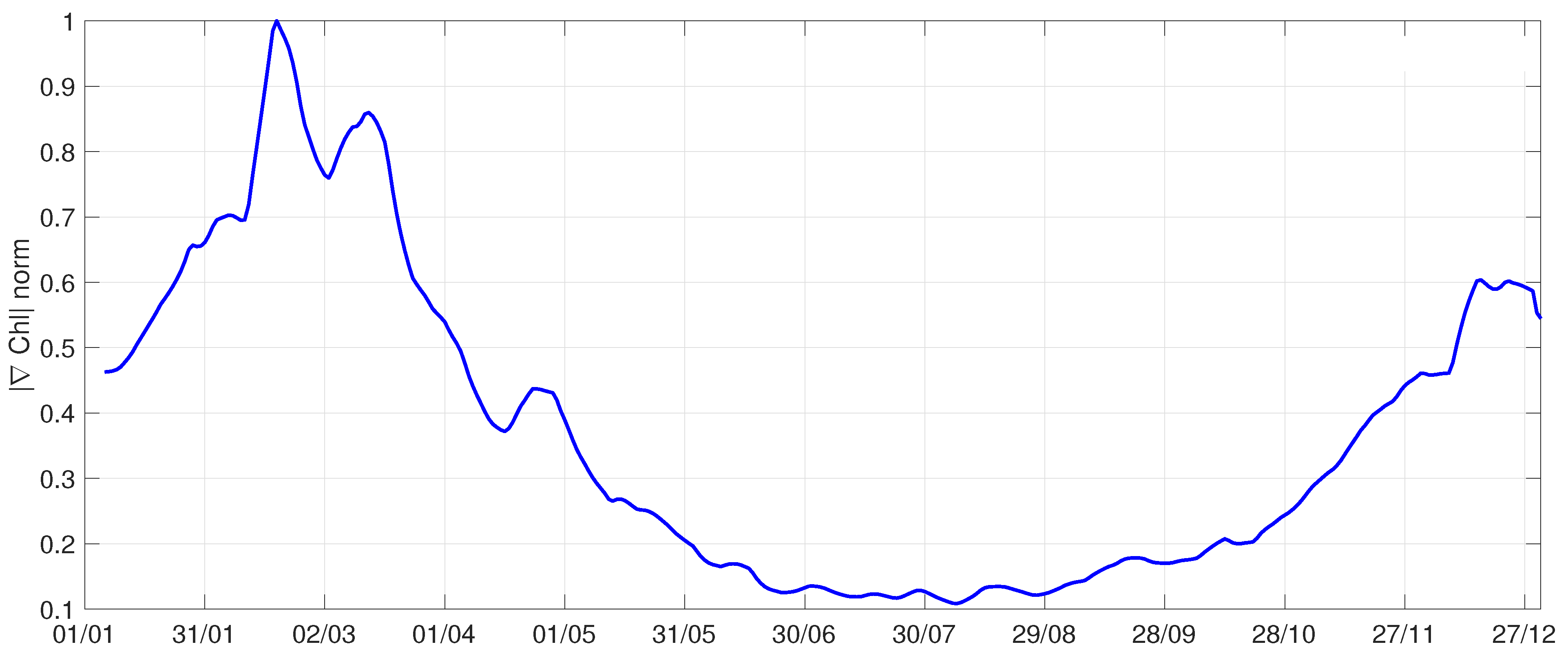
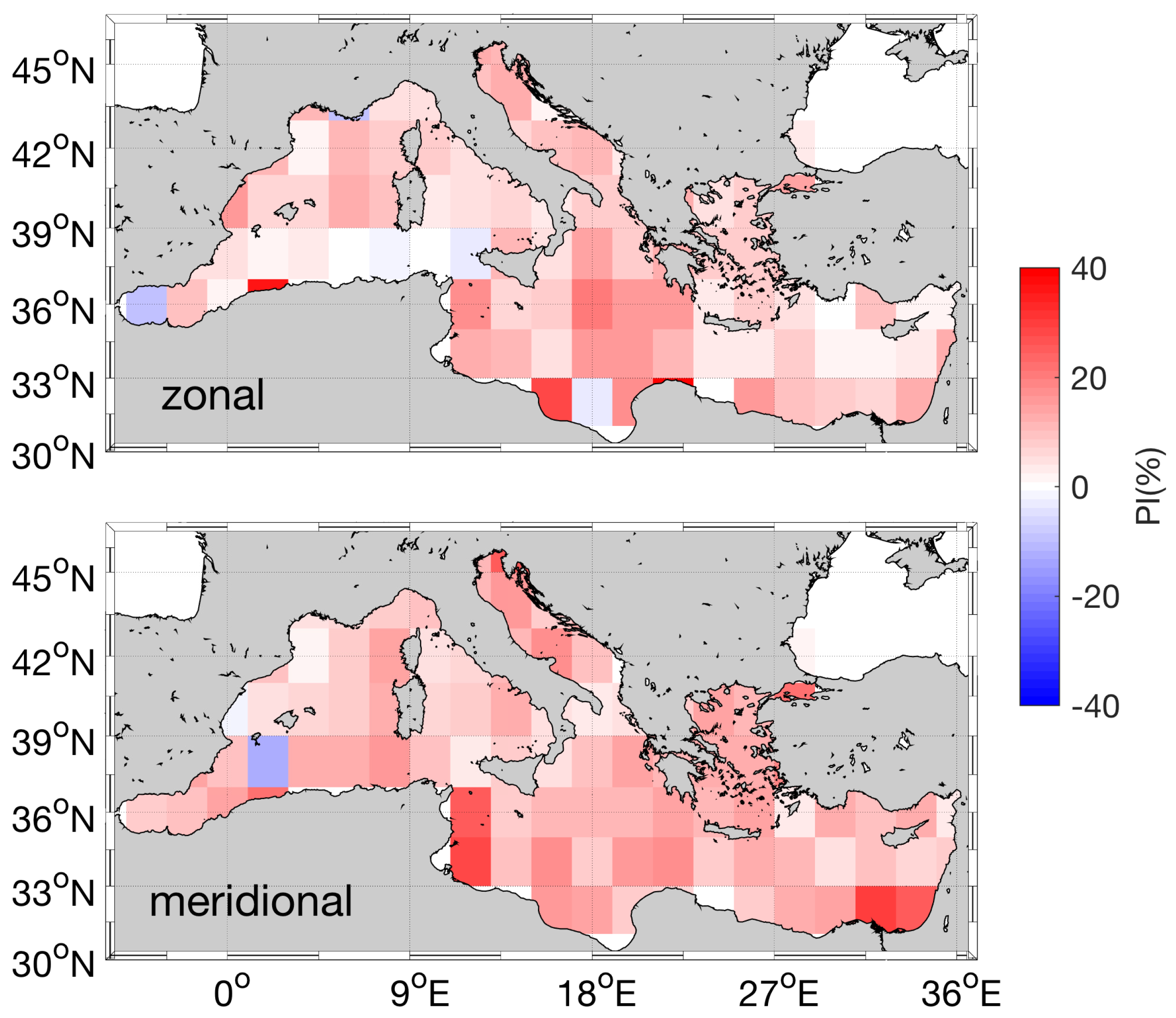
  • the optimal currents improve the surface circulation estimates provided by satellite altimetry by about 30 to 50% at the basin scale for both the zonal and meridional currents. This was determined checking simultaneously the RMSD values of the SAC and OPC with respect to the total surface currents estimates provided by the CMEMS PHY model. Such improvements can be found throughout the year. However, the enhanced biological activity during late winter/early spring [36,37] may give rise to significant changes in surface Chl gradients. Such gradients are not strictly related to the horizontal advection and can thus slightly reduce the OPC maximum improvements with respect to the altimeter system. The summer period (mostly late June/early July) can also give rise to issues in the optimal reconstruction: in this period, the Mediterranean sea surface Chl gradients reach their minimum value (evaluated via the CMEMS BIO model and shown in Figure 14 as a basin-scale average), preventing the optimal reconstruction (PIT09 method) to extract dynamical information from the surface tracer patterns;
  • the OPC built from Chl concentrations, despite Chl being obtained integrating contributions in the first tenths of meters of the water column, instead represent the surface circulation in the Mediterranean area.
The present-day Altimeter-derived gridded products in the Mediterranean Area fully resolve dynamical features at scales around 100 km and 10 days [21]. Therefore, extracting dynamical information from the patterns of the high-resolution Chl is advantageous to correct and improve the effective spatial-temporal resolution of such products.
Our study, however, has been carried out in a very idealized context. Relying on hydrodynamical and biogeochemical 3D models enables accessing full information on the Chl evolution that is used to constrain and correct the synthetic altimeter-derived currents. More in particular, this idealized framework allows for determining perfectly the source and sink terms that modulate the Chl variations at the sea surface, i.e., the F term of Equation (3), which is clearly much more complicated to account for in a realistic observational setup, due to complex biological responses and interactions within the surface layer. Indeed, the application of the PIT09 method to satellite-derived data will require approximating the forcing term from satellite information. Specific studies covering those aspects are already underway and will be the subject of future papers. Preliminary analyses on this topic seem to indicate that, at scales larger than 30 to 50 km, the F term is sufficiently well approximated by the temporal derivatives of the surface Chl field (F t Chl). An example is provided in Figure 15. During the main blooming events (mid-to-late February in our numerical study), the agreement between F and t Chl is only found at a large scale, while the smaller features O (20 km) cannot be retrieved exploiting the surface Chl temporal variations (Figure 15-left). Far from the blooming period, F and t Chl are mostly O (10 7 to 10 8 mg·m 3 ·s 1 ), i.e., one to two orders of magnitude lower than in the blooming period. The variability found in the F term is still given by the superposition of a large scale signal, the t Chl, and a small scale component (Figure 15-right).
Approximating the F term as t Chl means that the correction factors for the synthetic altimeter currents in Equation (4) are reduced to the case E = 0: the correction of the geostrophic current is only built accounting for the spatial derivatives of the surface Chl. As a result, we force the flow to follow the Chl concentration isolines. We check that this approximation (E = 0) still leads to satisfying statistical performances of the OPC (Figure 16).
The percentage of improvement of the SAC is computed throughout 2017 by means of Equation (5). Figure 16 depicts the zonal and meridional PI in 2 × 2 boxes. Given the approximation used here, the extent of the improvement is reduced compared to the idealized case, where the basin-scale PI could also exceed 50% in large Chl gradient areas (Figure 8). Here, the local improvements mostly range from 10 to 20% and, occasionally, degradations may occur in highly active dynamical areas such as the Alboran Sea or in correspondence with the Algerian Current.
This additional and preliminary analysis still encourages future applications of the PIT09 method with satellite-derived data, i.e., using only surface Chl and geostrophic currents fields, without the perfect knowledge of the daily forcing term. In such future analyses, the optimal reconstruction should also be implemented accounting for the uncertainties on the Forcing term, thus relying on the PIT09 set of equations used by [28,29,31]. In these studies, the uncertainties on the daily approximated forcing were computed by exploiting the high frequency (six-hourly to hourly) measurements of in situ SST by Lagrangian drifters [52,53]. This approach is not applicable for Chl, as the temporal sampling of in situ measurements of Chl is much lower than one day [54]. This could be addressed in the future by empowering the deployment of Lagrangian drifters designed for the measurements of high frequency sea surface bio-optical parameters (as presently achieved using Saildrones [55]). In the meantime, other approaches need to be explored, for instance relying on dedicated biogeochemical numerical simulations or exploiting machine learning techniques.
Future studies on the PIT09 method should also assess the potential of exploiting simultaneously different types of oceanic tracers like Chl and SST. Provided a good knowledge of the tracers’ evolution (including their source/sink terms), one could select the areas and periods where each tracer maximises the enhancement of the altimeter system capabilities. For instance, when surface Chl patterns are dominated by the biological activity, one could preferably rely on OPC estimates based on SST. Similarly, in case of prolonged uniform Chl fields (with tracer gradients close to zero), it could be useful to extract spatial-temporal gradients from SST fields, and vice versa [34].

Author Contributions

Conceptualization, D.C., B.B.N., M.-H.R. and R.S.; Data curation, E.C.; Formal analysis, D.C.; Funding acquisition, D.C. and R.S.; Investigation, D.C., E.C., B.B.N., M.-H.R. and R.S.; Methodology, D.C., B.B.N. and M.-H.R.; Project administration, D.C., M.-H.R. and R.S.; Resources, D.C. and R.S.; Software, D.C., E.C. and B.B.N.; Supervision, B.B.N., M.-H.R. and R.S.; Validation, E.C.; Writing—original draft, D.C., E.C. and B.B.N.; Writing—review and editing, E.C., B.B.N., M.-H.R. and R.S. All authors have read and agreed to the published version of the manuscript.

Funding

This work has been carried out as part of the CIRCOL (ocean CIRculation from ocean COLour observations) project, funded by the European Space Agency via the contract Grant No. 4000128147/19/I-DT.

Institutional Review Board Statement

Not Applicable.

Informed Consent Statement

Not Applicable.

Data Availability Statement

The data presented in this study are openly available via https://marine.copernicus.eu/ accessed on 13 May 2021 and http://circol.artov.ismar.cnr.it/products/PHASE1/ accessed on 13 May 2021.

Acknowledgments

The Authors thank the two anonymous Reviewers for providing valuable comments to improve our manuscript as well as hints for future studies. This paper also benefited from the help of Emanuela Clementi, who provided significant support on the CMEMS Mediterranean Sea Physics Analysis and Forecast model. Simone Colella and Gianluca Volpe are acknowledged for their continuous support and for the fruitful discussions. D.Ciani thanks Paolo Lazzari and Gianpiero Cossarini for the discussions on the analysis and forecast of the Mediterranean Sea biogeochemical state.

Conflicts of Interest

The authors declare no conflict of interest. The funders had no role in the design of the study; in the collection, analyses, or interpretation of data; in the writing of the manuscript, or in the decision to publish the results.

References

  1. Robinson, I.S. Measuring the Oceans from Space: The Principles and Methods of Satellite Oceanography; Springer: Berlin/Heidelberg, Germany, 2004. [Google Scholar]
  2. Bretherton, F.P.; Davis, R.E.; Fandry, C. A technique for objective analysis and design of oceanographic experiments applied to MODE-73. Deep Sea Res. Oceanogr. Abstr. 1976, 23, 559–582. [Google Scholar] [CrossRef]
  3. Le Traon, P.; Nadal, F.; Ducet, N. An improved mapping method of multisatellite altimeter data. J. Atmos. Ocean. Technol. 1998, 15, 522–534. [Google Scholar] [CrossRef]
  4. Donlon, C.J.; Martin, M.; Stark, J.; Roberts-Jones, J.; Fiedler, E.; Wimmer, W. The operational sea surface temperature and sea ice analysis (OSTIA) system. Remote Sens. Environ. 2012, 116, 140–158. [Google Scholar] [CrossRef]
  5. Reynolds, R.W.; Smith, T.M. Improved global sea surface temperature analyses using optimum interpolation. J. Clim. 1994, 7, 929–948. [Google Scholar] [CrossRef] [Green Version]
  6. Melnichenko, O.; Hacker, P.; Maximenko, N.; Lagerloef, G.; Potemra, J. Spatial optimal interpolation of Aquarius sea surface salinity: Algorithms and implementation in the North Atlantic. J. Atmos. Ocean. Technol. 2014, 31, 1583–1600. [Google Scholar] [CrossRef]
  7. Buongiorno Nardelli, B. A novel approach for the high-resolution interpolation of in situ sea surface salinity. J. Atmos. Ocean. Technol. 2012, 29, 867–879. [Google Scholar] [CrossRef]
  8. Buongiorno Nardelli, B.B.; Tronconi, C.; Pisano, A.; Santoleri, R. High and Ultra-High resolution processing of satellite Sea Surface Temperature data over Southern European Seas in the framework of MyOcean project. Remote Sens. Environ. 2013, 129, 1–16. [Google Scholar] [CrossRef]
  9. Droghei, R.; Buongiorno Nardelli, B.; Santoleri, R. A New Global Sea Surface Salinity and Density Dataset From Multivariate Observations (1993–2016). Front. Mar. Sci. 2018, 5, 84. [Google Scholar] [CrossRef] [Green Version]
  10. Beckers, J.M.; Rixen, M. EOF calculations and data filling from incomplete oceanographic datasets. J. Atmos. Ocean. Technol. 2003, 20, 1839–1856. [Google Scholar] [CrossRef]
  11. Volpe, G.; Nardelli, B.B.; Cipollini, P.; Santoleri, R.; Robinson, I.S. Seasonal to interannual phytoplankton response to physical processes in the Mediterranean Sea from satellite observations. Remote Sens. Environ. 2012, 117, 223–235. [Google Scholar] [CrossRef]
  12. Krasnopolsky, V.; Nadiga, S.; Mehra, A.; Bayler, E.; Behringer, D. Neural networks technique for filling gaps in satellite measurements: Application to ocean color observations. Comput. Intell. Neurosci. 2016, 2016, 6156513. [Google Scholar] [CrossRef] [Green Version]
  13. Bolton, T.; Zanna, L. Applications of deep learning to ocean data inference and subgrid parameterization. J. Adv. Model. Earth Syst. 2019, 11, 376–399. [Google Scholar] [CrossRef] [Green Version]
  14. Barth, A.; Alvera Azcarate, A.; Licer, M.; Beckers, J.M. DINCAE 1.0: A convolutional neural network with error estimates to reconstruct sea surface temperature satellite observations. Geosci. Model Dev. 2020, 13, 1609–1622. [Google Scholar] [CrossRef] [Green Version]
  15. Cancet, M.; Griffin, D.; Cahill, M.; Chapron, B.; Johannessen, J.; Donlon, C. Evaluation of GlobCurrent surface ocean current products: A case study in Australia. Remote Sens. Environ. 2019, 220, 71–93. [Google Scholar] [CrossRef] [Green Version]
  16. Liu, Y.; Weisberg, R.H.; Vignudelli, S.; Mitchum, G.T. Evaluation of altimetry-derived surface current products using Lagrangian drifter trajectories in the eastern Gulf of Mexico. J. Geophys. Res. Ocean. 2014, 119, 2827–2842. [Google Scholar] [CrossRef] [Green Version]
  17. Pujol, M.I.; Dibarboure, G.; Le Traon, P.Y.; Klein, P. Using high-resolution altimetry to observe mesoscale signals. J. Atmos. Ocean. Technol. 2012, 29, 1409–1416. [Google Scholar] [CrossRef]
  18. Pujol, M.I.; Faugère, Y.; Taburet, G.; Dupuy, S.; Pelloquin, C.; Ablain, M.; Picot, N. DUACS DT2014: The new multi-mission altimeter data set reprocessed over 20 years. Ocean Sci. 2016, 12, 1067–1090. [Google Scholar] [CrossRef] [Green Version]
  19. Pascual, A.; Faugère, Y.; Larnicol, G.; Le Traon, P.Y. Improved description of the ocean mesoscale variability by combining four satellite altimeters. Geophys. Res. Lett. 2006, 33. [Google Scholar] [CrossRef] [Green Version]
  20. Taburet, G.; Sanchez-Roman, A.; Ballarotta, M.; Pujol, M.I.; Legeais, J.F.; Fournier, F.; Faugere, Y.; Dibarboure, G. DUACS DT2018: 25 years of reprocessed sea level altimetry products. Ocean Sci. 2019, 15, 1207–1224. [Google Scholar] [CrossRef] [Green Version]
  21. Ballarotta, M.; Ubelmann, C.; Pujol, M.I.; Taburet, G.; Fournier, F.; Legeais, J.F.; Faugère, Y.; Delepoulle, A.; Chelton, D.; Dibarboure, G.; et al. On the resolutions of ocean altimetry maps. Ocean Sci. 2019, 15, 1091–1109. [Google Scholar] [CrossRef] [Green Version]
  22. Fu, L.L.; Ferrari, R. Observing oceanic submesoscale processes from space. Eos Trans. Am. Geophys. Union 2008, 89, 488. [Google Scholar] [CrossRef]
  23. Ubelmann, C.; Klein, P.; Fu, L.L. Dynamic interpolation of sea surface height and potential applications for future high-resolution altimetry mapping. J. Atmos. Ocean. Technol. 2015, 32, 177–184. [Google Scholar] [CrossRef] [Green Version]
  24. Ballarotta, M.; Ubelmann, C.; Rogé, M.; Fournier, F.; Faugère, Y.; Dibarboure, G.; Morrow, R.; Picot, N. Dynamic Mapping of Along-Track Ocean Altimetry: Performance from Real Observations. J. Atmos. Ocean. Technol. 2020, 37, 1593–1601. [Google Scholar] [CrossRef]
  25. Mulet, S.; Etienne, H.; Ballarotta, M.; Faugere, Y.; Rio, M.; Dibarboure, G.; Picot, N. Synergy between surface drifters and altimetry to increase the accuracy of sea level anomaly and geostrophic current maps in the Gulf of Mexico. Adv. Space Res. 2020, 68, 420–431. [Google Scholar] [CrossRef]
  26. Piterbarg, L.I. A simple method for computing velocities from tracer observations and a model output. Appl. Math. Model. 2009, 33, 3693–3704. [Google Scholar] [CrossRef]
  27. Rio, M.H.; Santoleri, R.; Bourdalle-Badie, R.; Griffa, A.; Piterbarg, L.; Taburet, G. Improving the Altimeter-Derived Surface Currents Using High-Resolution Sea Surface Temperature Data: A Feasability Study Based on Model Outputs. J. Atmos. Ocean. Technol. 2016, 33, 2769–2784. [Google Scholar] [CrossRef]
  28. Rio, M.H.; Santoleri, R. Improved global surface currents from the merging of altimetry and Sea Surface Temperature data. Remote Sens. Environ. 2018, 216, 770–785. [Google Scholar] [CrossRef]
  29. Ciani, D.; Rio, M.H.; Menna, M.; Santoleri, R. A Synergetic Approach for the Space-Based Sea Surface Currents Retrieval in the Mediterranean Sea. Remote Sens. 2019, 11, 1285. [Google Scholar] [CrossRef] [Green Version]
  30. Menna, M.; Poulain, P.M.; Ciani, D.; Doglioli, A.; Notarstefano, G.; Gerin, R.; Rio, M.H.; Santoleri, R.; Gauci, A.; Drago, A. New insights of the Sicily Channel and southern Tyrrhenian Sea variability. Water 2019, 11, 1355. [Google Scholar] [CrossRef] [Green Version]
  31. Ciani, D.; Rio, M.H.; Nardelli, B.B.; Etienne, H.; Santoleri, R. Improving the Altimeter-Derived Surface Currents Using Sea Surface Temperature (SST) Data: A Sensitivity Study to SST Products. Remote Sens. 2020, 12, 1601. [Google Scholar] [CrossRef]
  32. Warren, M.; Quartly, G.; Shutler, J.; Miller, P.; Yoshikawa, Y. Estimation of ocean surface currents from maximum cross correlation applied to GOCI geostationary satellite remote sensing data over the Tsushima (Korea) Straits. J. Geophys. Res. Ocean. 2016, 121, 6993–7009. [Google Scholar] [CrossRef] [Green Version]
  33. Li, G.; He, Y.; Liu, G.; Zhang, Y.; Hu, C.; Perrie, W. Multi-Sensor Observations of Submesoscale Eddies in Coastal Regions. Remote Sens. 2020, 12, 711. [Google Scholar] [CrossRef] [Green Version]
  34. Liu, Y.; Weisberg, R.H.; Hu, C.; Kovach, C.; Riethmüller, R. Evolution of the Loop Current system during the Deepwater Horizon oil spill event as observed with drifters and satellites. Monit. Model. Deep. Horiz. Oil Spill Rec.-Break. Enterp. Geophys. Monogr. Ser. 2011, 195, 91–101. [Google Scholar]
  35. Levy, M.; Martin, A. The influence of mesoscale and submesoscale heterogeneity on ocean biogeochemical reactions. Glob. Biogeochem. Cycles 2013, 27, 1139–1150. [Google Scholar] [CrossRef] [Green Version]
  36. Malanotte-Rizzoli, P.; The Pan-Med Group. Physical forcing and physical/biochemical variability of the Mediterranean Sea: A review of unresolved issues and directions of future research. Ocean Sci. 2014, 10, 281–322. [Google Scholar] [CrossRef] [Green Version]
  37. d’Ortenzio, F.; d’Alcalà, M.R. On the trophic regimes of the Mediterranean Sea: A satellite analysis. Biogeosciences 2009, 6, 139–148. [Google Scholar] [CrossRef] [Green Version]
  38. Mayot, N.; D’Ortenzio, F.; d’Alcala, M.R.; Lavigne, H.; Claustre, H. Interannual variability of the Mediterranean trophic regimes from ocean color satellites. Biogeosciences 2016, 13, 1901–1917. [Google Scholar] [CrossRef] [Green Version]
  39. Clementi, E.; Pistoia, J.; Escudier, R.; Delrosso, D.; Drudi, M.; Grandi, A.; Lecci, R.; Cretí, S.; Ciliberti, S.A.; Coppini, G.; et al. Mediterranean Sea Analysis and Forecast (CMEMS MED-Currents EAS5 System) [Data Set]; Copernicus Monitoring Environment Marine Service (CMEMS): Lecce, Italy, 2019. [Google Scholar]
  40. Lazzari, P.; Solidoro, C.; Ibello, V.; Salon, S.; Teruzzi, A.; Béranger, K.; Colella, S.; Crise, A. Seasonal and inter-annual variability of plankton chlorophyll and primary production in the Mediterranean Sea: A modelling approach. Biogeosciences 2012, 9, 217–233. [Google Scholar] [CrossRef] [Green Version]
  41. Lazzari, P.; Solidoro, C.; Salon, S.; Bolzon, G. Spatial variability of phosphate and nitrate in the Mediterranean Sea: A modeling approach. Deep Sea Res. Part I Oceanogr. Res. Pap. 2016, 108, 39–52. [Google Scholar] [CrossRef] [Green Version]
  42. Cossarini, G.; Querin, S.; Solidoro, C.; Sannino, G.; Lazzari, P.; Di Biagio, V.; Bolzon, G. Development of BFMCOUPLER (v1.0), the coupling scheme that links the MITgcm and BFM models for ocean biogeochemistry simulations. Geosci. Model Dev. 2017, 10, 1423–1445. [Google Scholar] [CrossRef] [Green Version]
  43. Carrère, L.; Lyard, F. Modeling the barotropic response of the global ocean to atmospheric wind and pressure forcing-comparisons with observations. Geophys. Res. Lett. 2003, 30. [Google Scholar] [CrossRef] [Green Version]
  44. Gaultier, L.; Ubelmann, C.; Fu, L.L. The challenge of using future SWOT data for oceanic field reconstruction. J. Atmos. Ocean. Technol. 2016, 33, 119–126. [Google Scholar] [CrossRef]
  45. Morel, A.; Berthon, J.F. Surface pigments, algal biomass profiles, and potential production of the euphotic layer: Relationships reinvestigated in view of remote-sensing applications. Limnol. Oceanogr. 1989, 34, 1545–1562. [Google Scholar] [CrossRef] [Green Version]
  46. Barbieux, M.; Uitz, J.; Gentili, B.; Pasqueron de Fommervault, O.; Mignot, A.; Poteau, A.; Schmechtig, C.; Taillandier, V.; Leymarie, E.; Penkerc’h, C.; et al. Bio-optical characterization of subsurface chlorophyll maxima in the Mediterranean Sea from a Biogeochemical-Argo float database. Biogeosciences 2019, 16, 1321–1342. [Google Scholar] [CrossRef] [Green Version]
  47. Vichi, M.; Lovato, T.; Mlot, E.G.; McKiver, W. Coupling BFM with Ocean Models, Nucleus for the European Modelling of the Ocean, Release 1.0; BFM: Bologna, Italy, 2015. [Google Scholar] [CrossRef]
  48. Ruiz, S.; Claret, M.; Pascual, A.; Olita, A.; Troupin, C.; Capet, A.; Tovar-Sánchez, A.; Allen, J.; Poulain, P.M.; Tintoré, J.; et al. Effects of oceanic mesoscale and submesoscale frontal processes on the vertical transport of phytoplankton. J. Geophys. Res. Ocean. 2019, 124, 5999–6014. [Google Scholar] [CrossRef] [Green Version]
  49. Buongiorno Nardelli, B. Vortex waves and vertical motion in a mesoscale cyclonic eddy. J. Geophys. Res. Ocean. 2013, 118, 5609–5624. [Google Scholar] [CrossRef]
  50. Nardelli, B.B.; Droghei, R.; Santoleri, R. Multi-dimensional interpolation of SMOS sea surface salinity with surface temperature and in situ salinity data. Remote Sens. Environ. 2016, 180, 392–402. [Google Scholar] [CrossRef]
  51. Vallis, G.K. Atmospheric and Oceanic Fluid Dynamics; Cambridge University Press: Cambridge, UK, 2006; p. 745. [Google Scholar]
  52. Menna, M.; Poulain, P.M.; Bussani, A.; Gerin, R. Detecting the drogue presence of SVP drifters from wind slippage in the Mediterranean Sea. Measurement 2018, 125, 447–453. [Google Scholar] [CrossRef]
  53. Lumpkin, R.; Özgökmen, T.; Centurioni, L. Advances in the application of surface drifters. Annu. Rev. Mar. Sci. 2017, 9, 59–81. [Google Scholar] [CrossRef] [Green Version]
  54. Claustre, H.; Bishop, J.; Boss, E.; Bernard, S.; Berthon, J.F.; Coatanoan, C.; Johnson, K.; Lotiker, A.; Ulloa, O.; Perry, M.J.; et al. Bio-optical profiling floats as new observational tools for biogeochemical and ecosystem studies: Potential synergies with ocean color remote sensing. In Proceedings of the OceanObs’09: Sustained Ocean Observations and Information for Society, Venice, Italy, 21–25 September 2009. [Google Scholar]
  55. Scott, J.P.; Crooke, S.; Cetinić, I.; Del Castillo, C.E.; Gentemann, C.L. Correcting non-photochemical quenching of Saildrone chlorophyll-a fluorescence for evaluation of satellite ocean color retrievals. Opt. Express 2020, 28, 4274–4285. [Google Scholar] [CrossRef] [PubMed]
Figure 1. (Left) Normalized scatter density plots between Chl-1m and C sat . (Left) high biological production period, 20 February to 20 March 2017. (Right) low biological production period, 15 July to 15 August 2017. In both panels, the identity line is given in blue.
Remotesensing 13 02389 g001
Figure 2. Workflow of the OSSE, covering the entire year 2017.
Remotesensing 13 02389 g002
Figure 3. (A) Northwestern Mediterranean: left, middle and right panels, respectively, indicate the Synthetic Altimeter Currents (SAC), Optimal Currents (OPC) and CMEMS PHY modelled currents. (B) same as (A), with focus on the Sicily Channel. (C) same as (A), with focus on the Western Mediterranean.
Remotesensing 13 02389 g003
Figure 4. Surface Chl from the CMEMS MedBFM BIO model in: (A) the Northwestern Mediterranean, (C) the Sicily Channel, (E) the Western Mediterranean. (B,D,F) Chl spatial gradients magnitude | Chl |, same areas as (A,C,E), respectively.
Remotesensing 13 02389 g004
Figure 5. Correction factors for the zonal SACs in: (A) the Northwestern Mediterranean; (C) the Sicily Channel; (E) the Western Mediterranean; (B,D,F) the same as (A,C,E) for the meridional SACs.
Remotesensing 13 02389 g005
Figure 6. (Left) column: RMSDs of the Synthetic Altimeter Currents (SAC) against the CMEMS PHY outputs, top and bottom panels show results for the zonal and the meridional currents. (Right) column: same as the left column, for the OPtimal Currents (OPC).
Remotesensing 13 02389 g006
Figure 7. Distributions of the RMSD values for the SAC (light green) and OPC (blue). Left and right panels show the results for the zonal and meridional currents, respectively.
Remotesensing 13 02389 g007
Figure 8. (Left) improvement of the zonal (blue) and meridional (red) optimal currents with respect to the Synthetic Altimeter estimates (January to Mid-February and Mid-March to December 2017). (Right) same as left, in the period mid-February to mid-March 2017.
Remotesensing 13 02389 g008
Figure 9. Temporal standard deviation (STD) of the CMEMS PHY and optimal surface currents for the year 2017. (Top) CMEMS PHY STD; (Middle) STD of the optimal currents (OPC); (Bottom) Δ STD: differences between the OPC and the Synthetic Altimeter Currents (SAC) STDs. (Left) and (right) columns stand for zonal and meridional currents, respectively.
Remotesensing 13 02389 g009
Figure 10. Differences between the OPC and the SAC temporal standard deviations ( Δ STD) computed on a 10-day temporal window. (Left) and (right) panels stand for zonal and meridional currents, respectively.
Remotesensing 13 02389 g010
Figure 11. Kinetic energy power spectral density of the Synthetic Altimeter Currents (SAC, red), OPtimal currents (OPC, blue) and CMEMS PHY modelled currents (light blue). The spectra are computed in the WEST and EAST areas of the Mediterranean, depicted by the yellow and green borders, respectively.
Remotesensing 13 02389 g011
Figure 12. Maximum OPC basin scale averaged PI over the year 2017, seen as a function of depth.
Remotesensing 13 02389 g012
Figure 13. Depth of maximum OPC PI over the year 2017, represented in 1 × 1 boxes.
Remotesensing 13 02389 g013
Figure 14. Temporal evolution of the spatial Chl gradient magnitude ( | Chl | , normalized).
Remotesensing 13 02389 g014
Figure 15. (Left) Top panel represents the F term computed by means of Equation (3). The bottom panel shows the surface Chl temporal derivative on 16 February 2017. (Right) same analyses reproduced on 25 July 2017.
Remotesensing 13 02389 g015
Figure 16. PI of the Optimal Currents given in 2 × 2 boxes: (top) zonal currents; (bottom) meridional currents.
Remotesensing 13 02389 g016
Table 1. Mean 1 Hz noise measurement observed for the different altimeters on along-track (L3) DUACS products in the Mediterranean Sea. Noise for raw SLA is indicated in cm rms.
MissionNoise Measurement Error
Jason-32.4
Sentinel-3A2.1
SARAL/AltiKa1.75
Cryosat-22.1
Publisher’s Note: MDPI stays neutral with regard to jurisdictional claims in published maps and institutional affiliations.

