
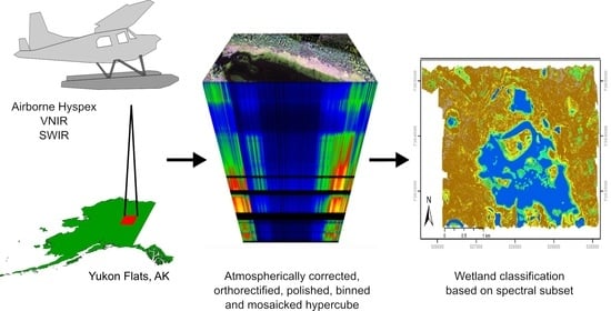
Airborne Hyperspectral Data Acquisition and Processing in the Arctic: A Pilot Study Using the Hyspex Imaging Spectrometer for Wetland Mapping


 , ,
, ,
Abstract
:
1. Introduction
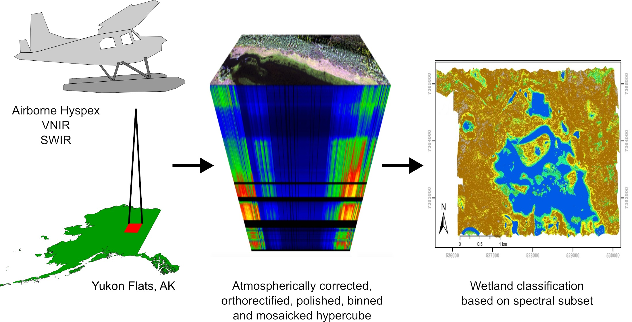
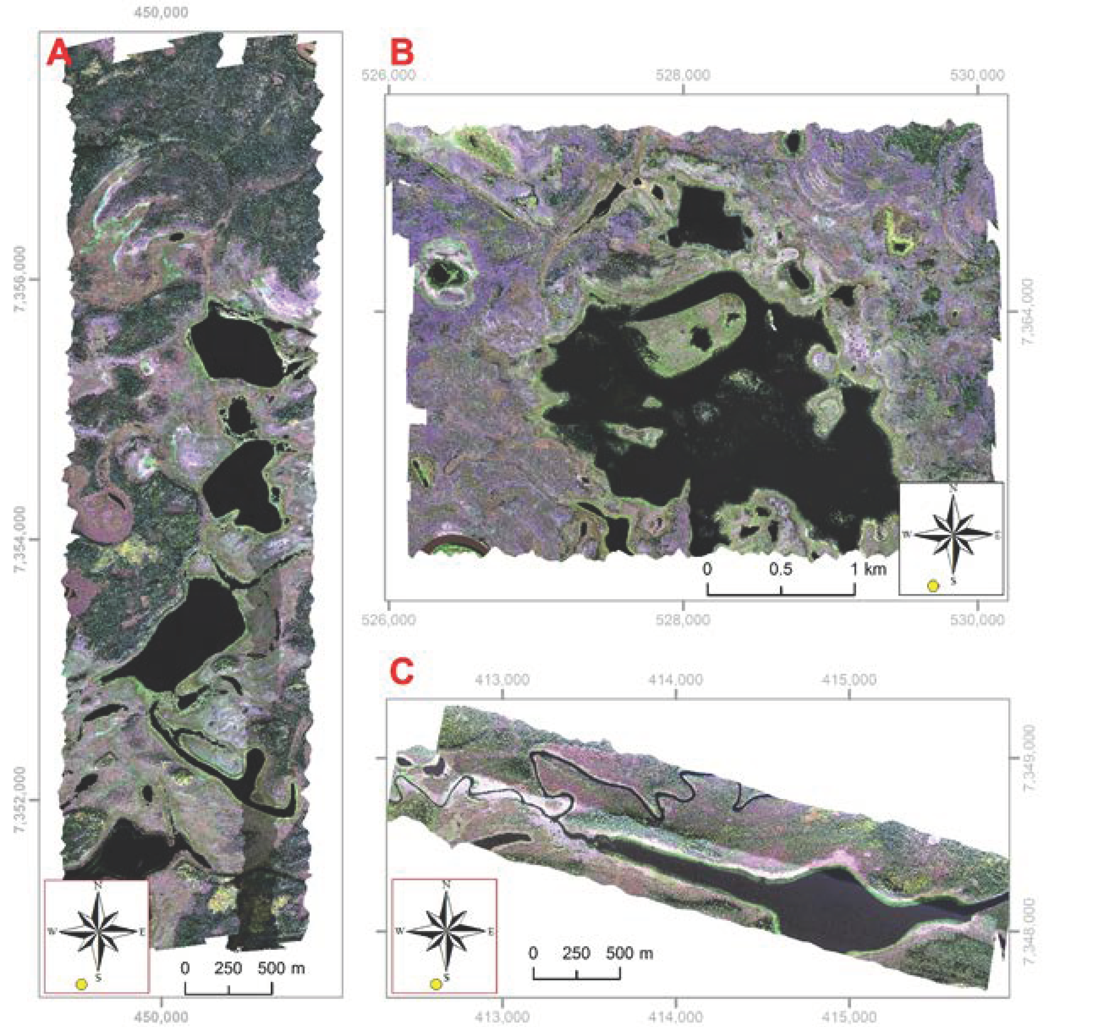
2. Study Area
3. HySpex System Commissioning and Data Acquisition
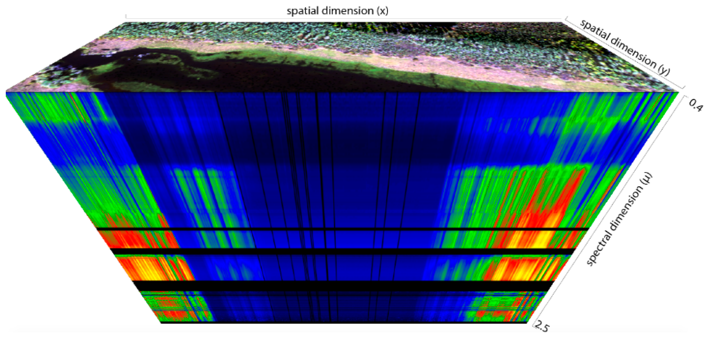
3.1. HySpex Hyperspectral Imaging System
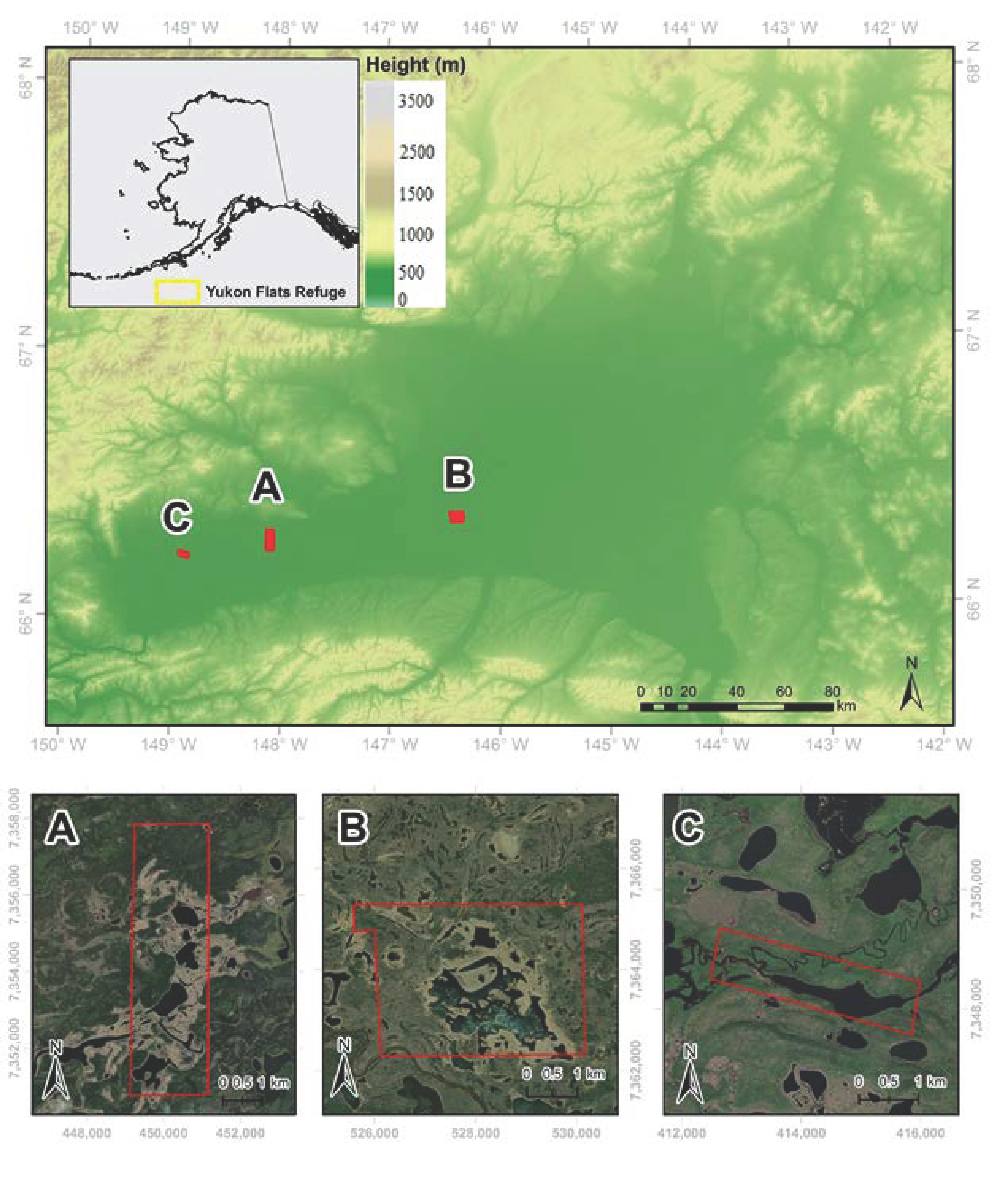
3.2. Integration of HySpex into Aircraft
3.3. Flight Planning and Data Acquisition
4. Hyperspectral Data Processing
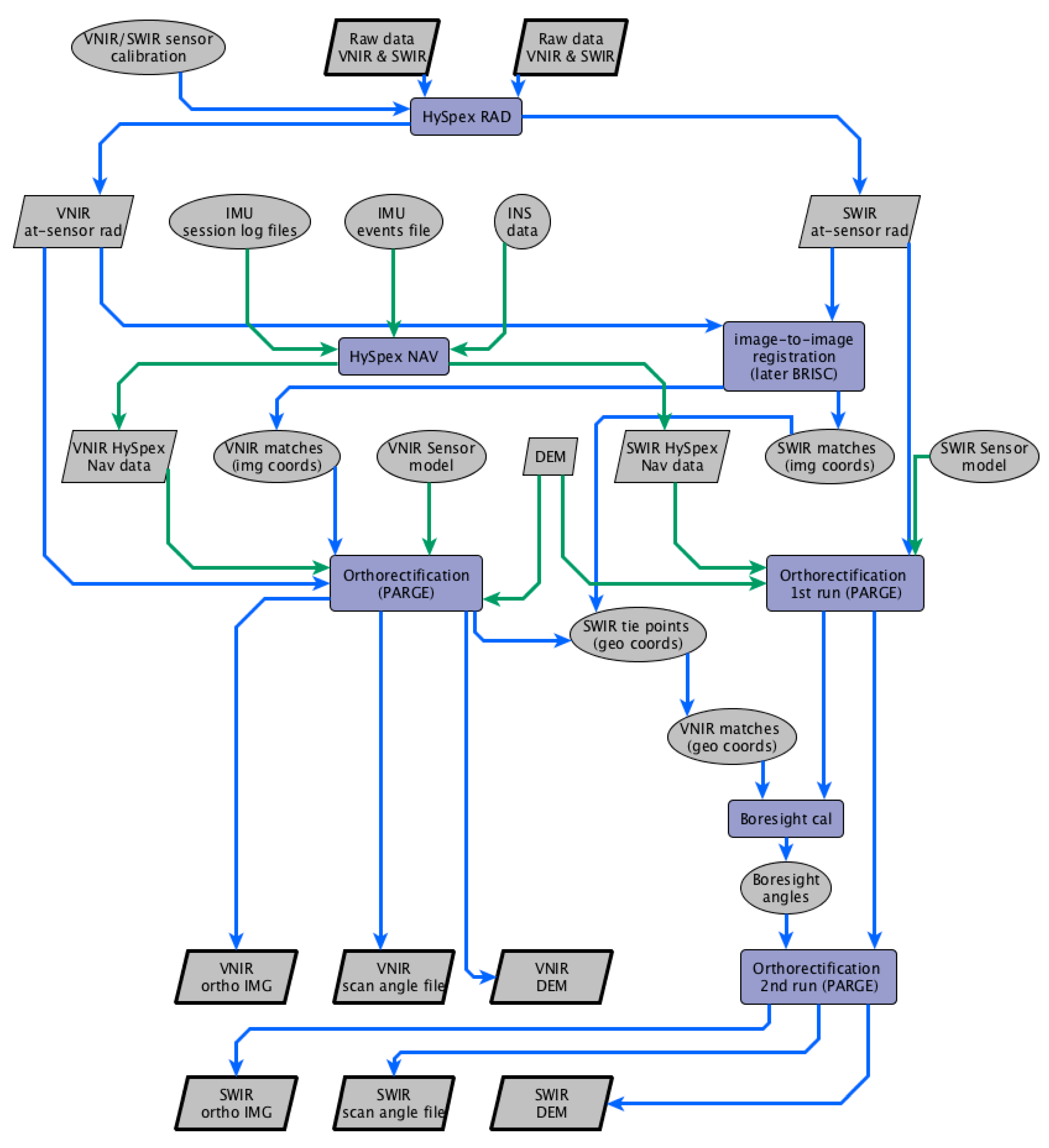
4.1. Raw Images to At-Sensor Radiance Images
4.2. Image Orthorectification
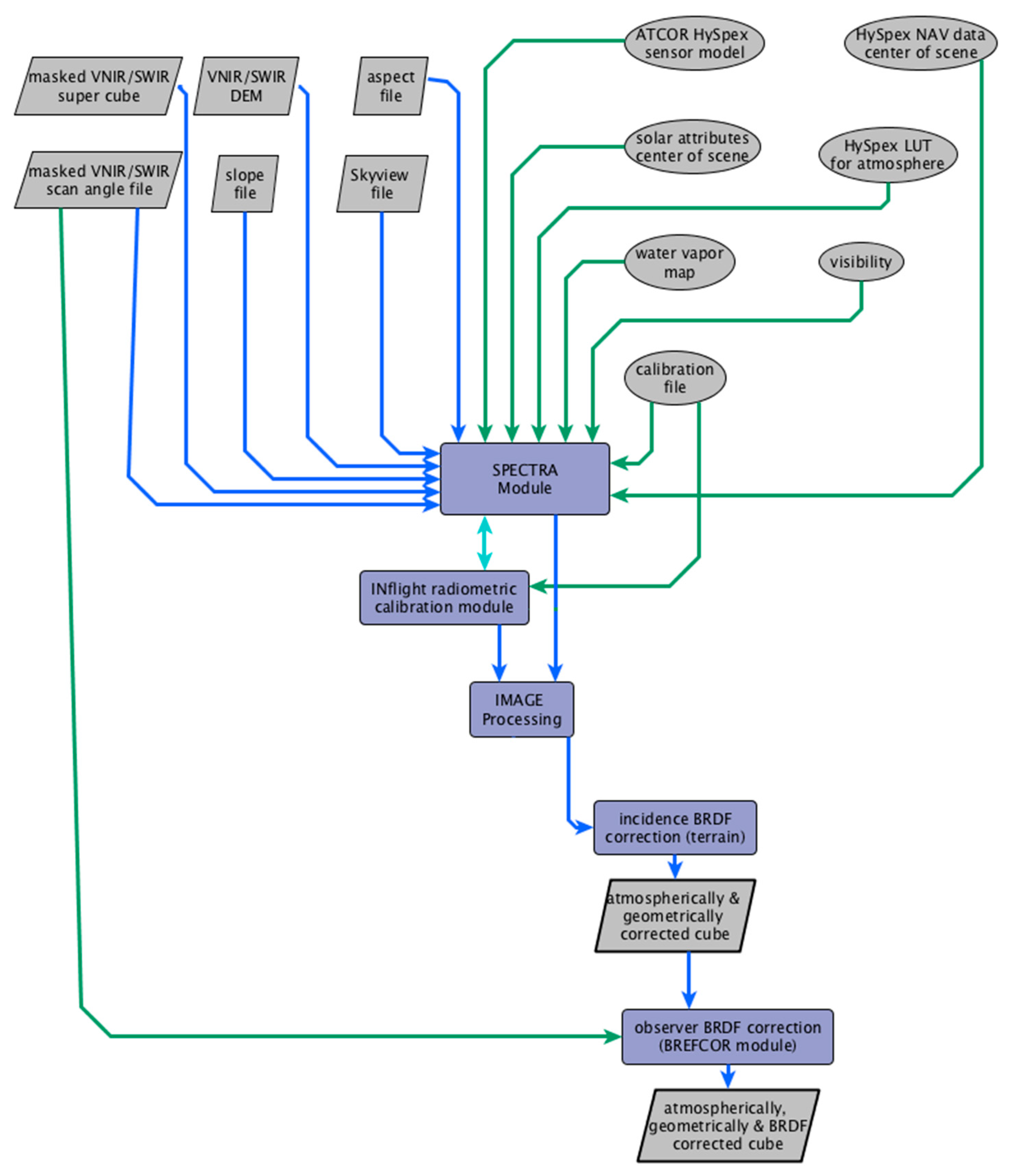
4.3. Radiometric Correction
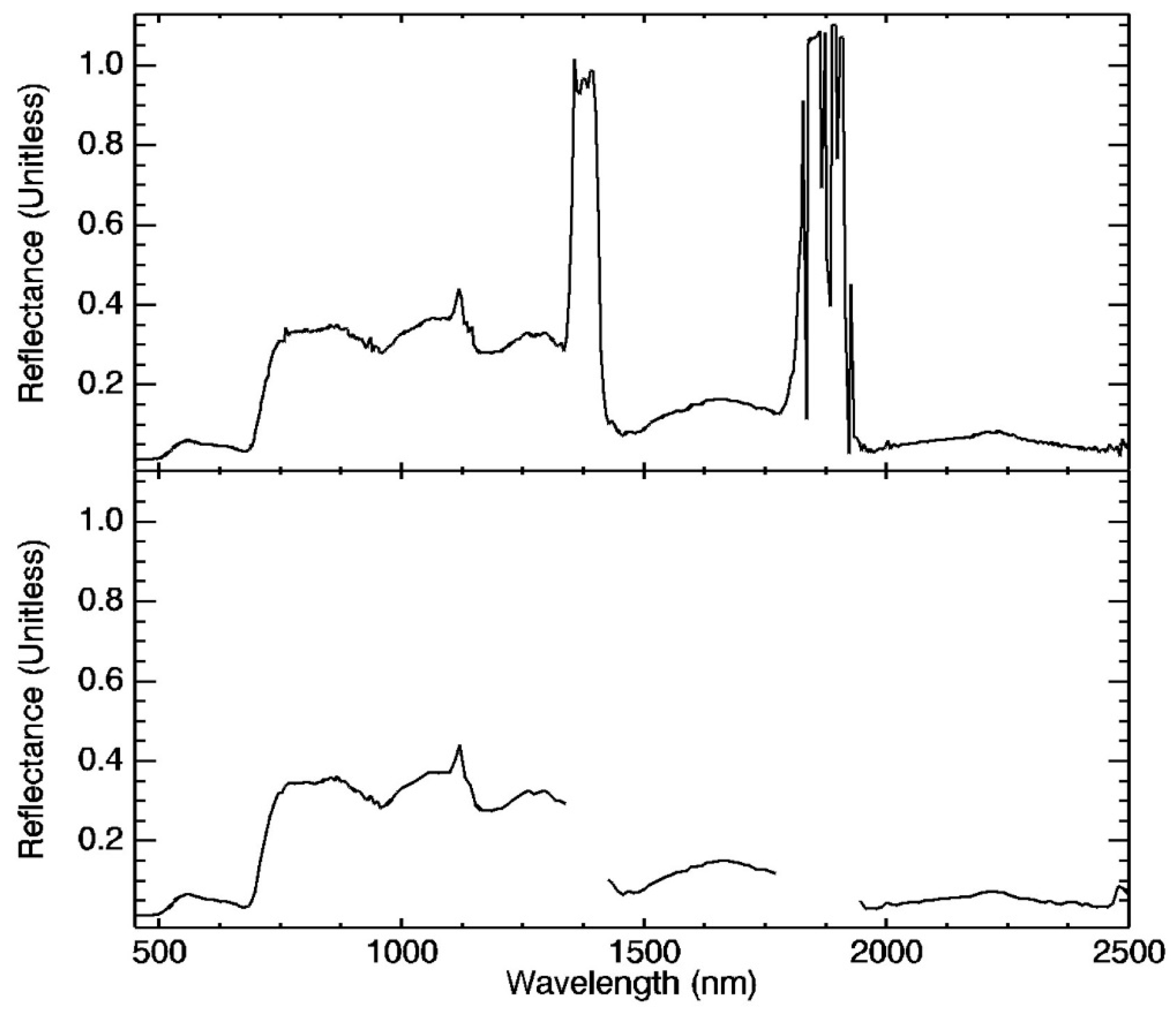
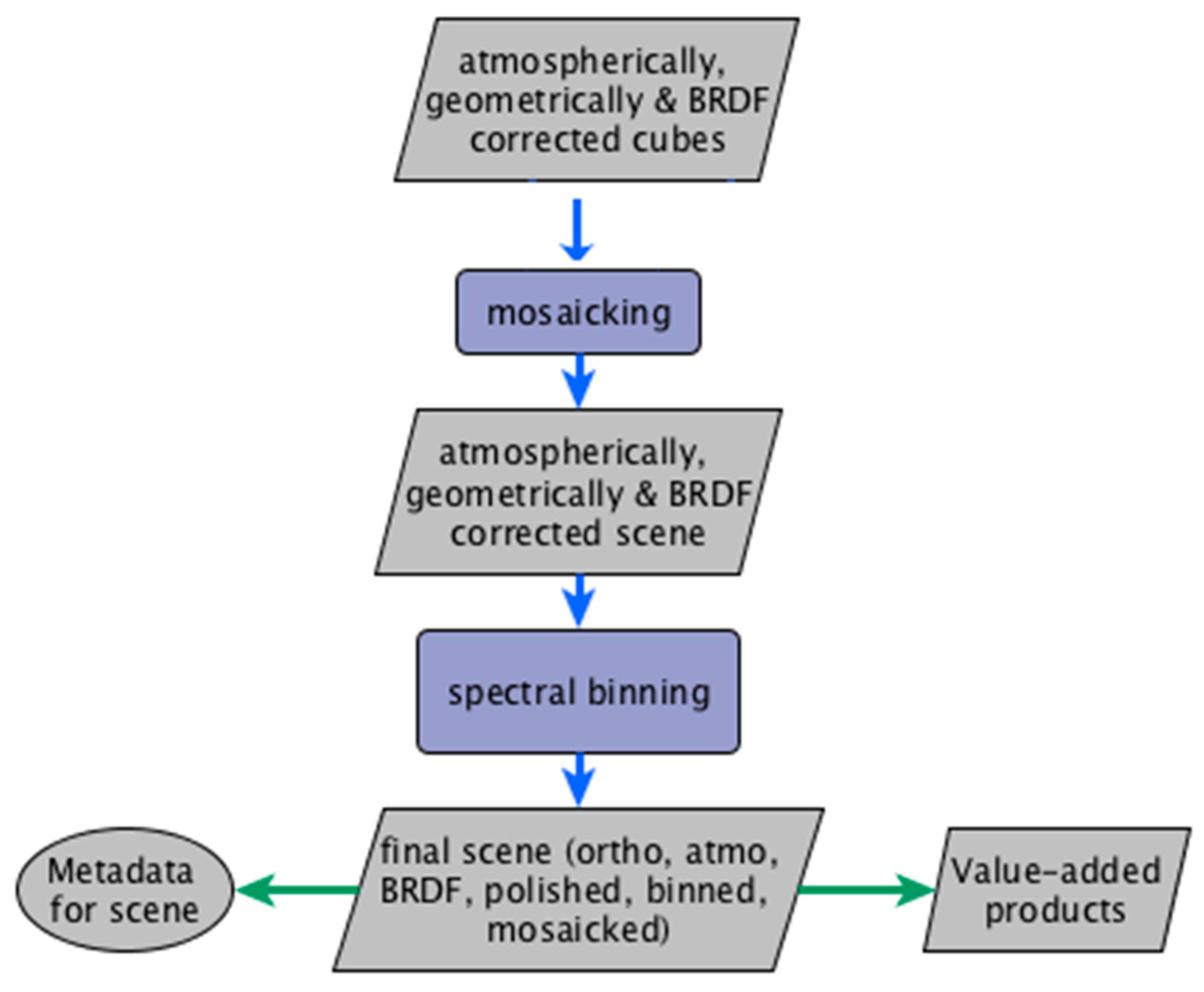
4.4. Spectral Binning and Final Mosaic
5. Wetland Mapping
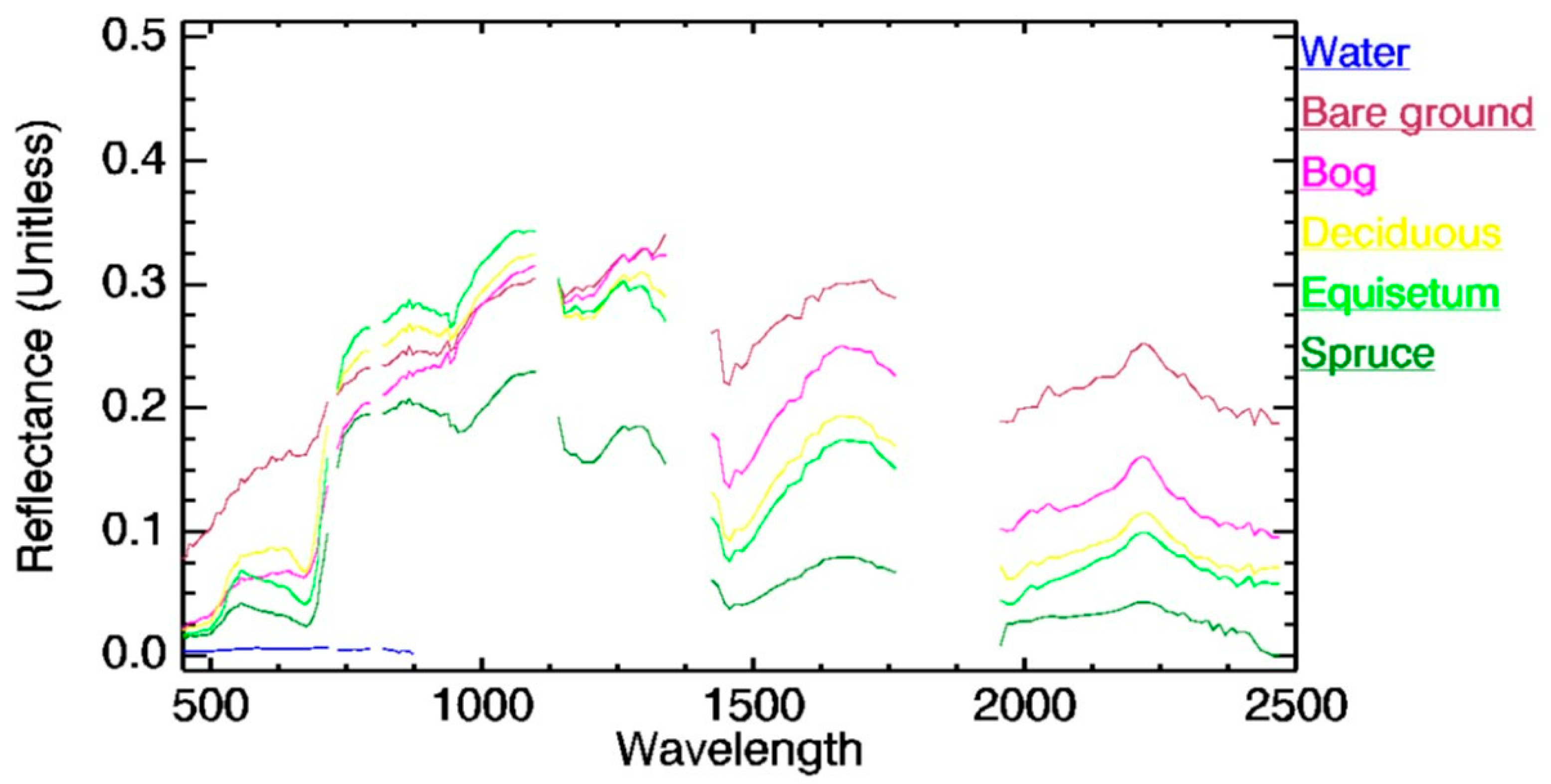
5.1. Category Definition
5.2. Training and Test Areas Selection and Band Selection
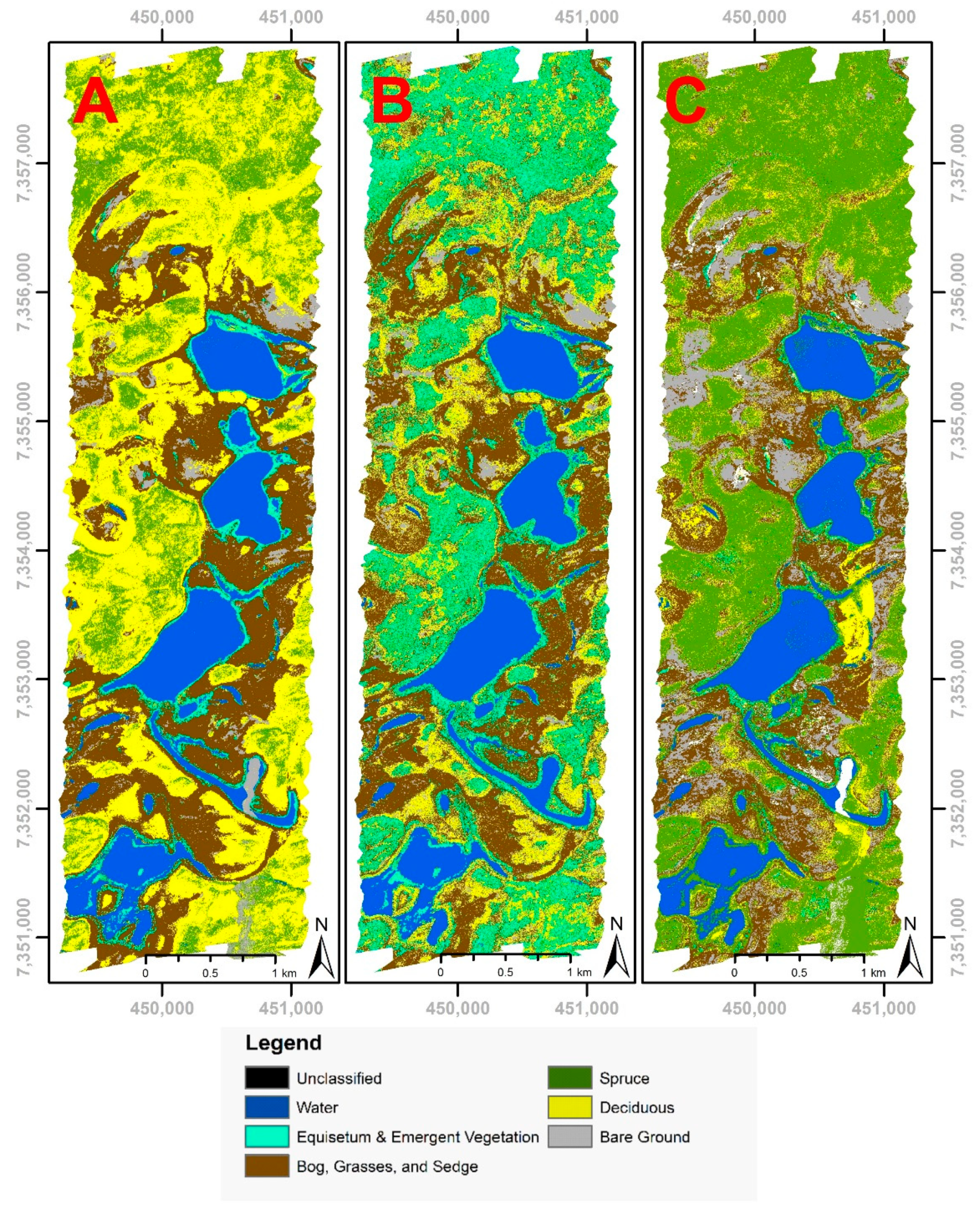
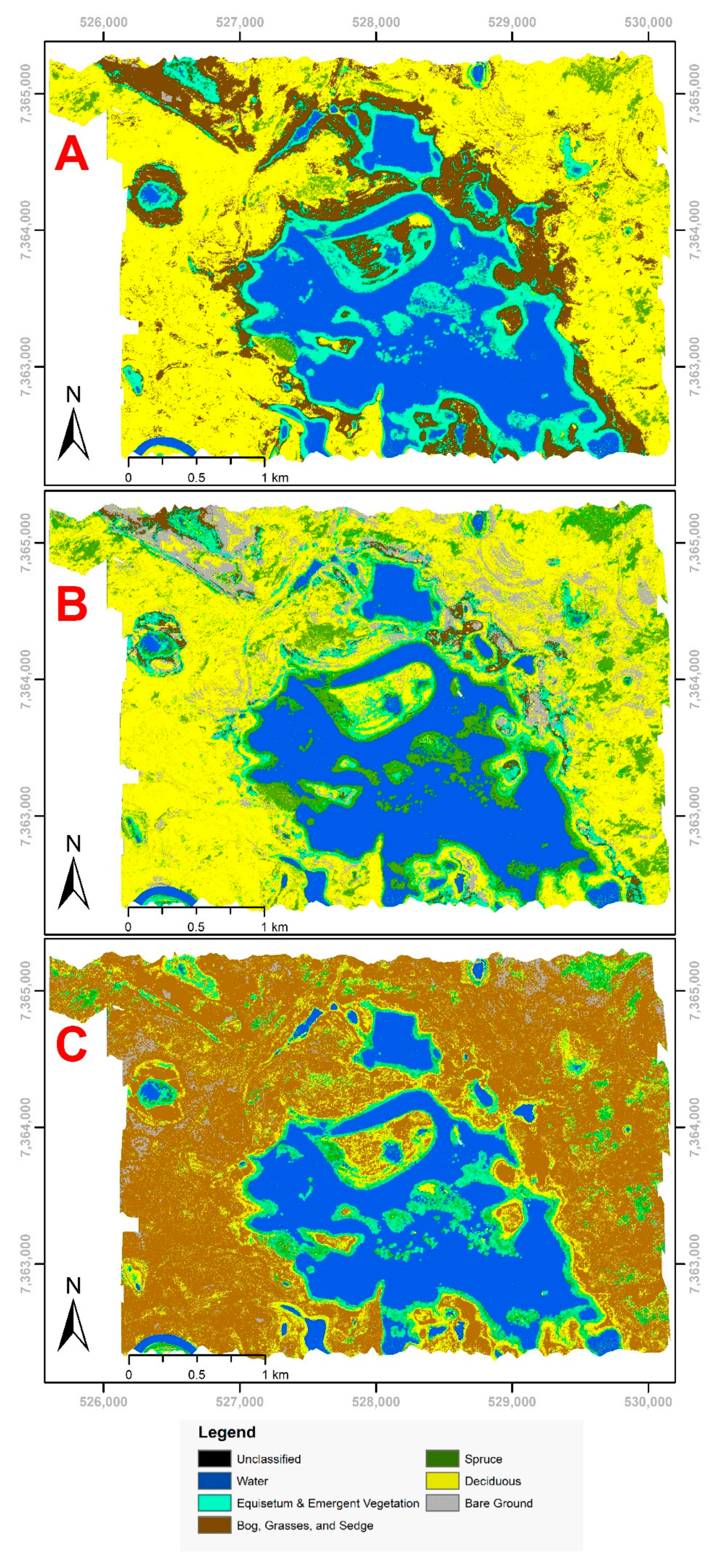
5.3. Image Classification Methods: Hybrid Classification, Maximum Likelihood and Spectral Angle Mapper (SAM)
6. Results and Discussion
6.1. Commissioning and Data Acquisition
6.2. Image Processing
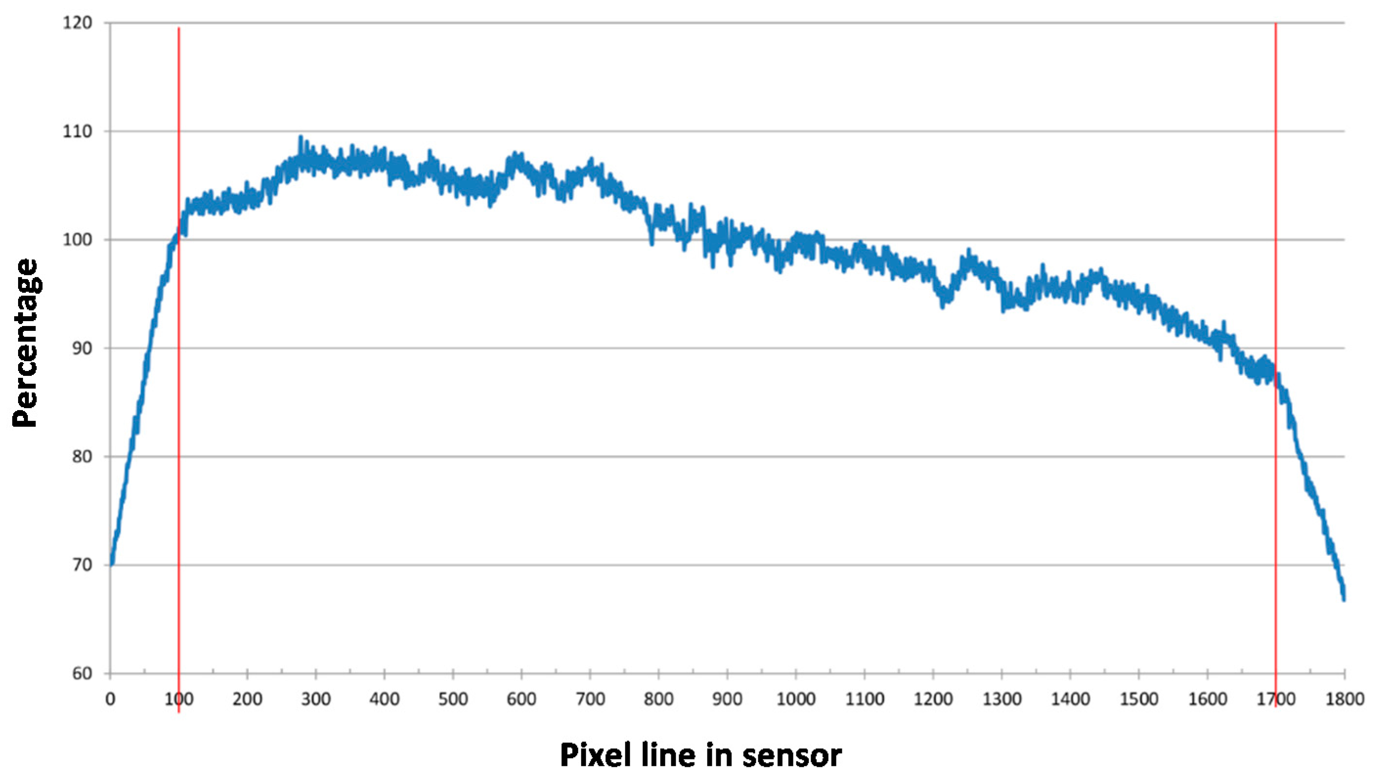
6.2.1. Systematic VNIR Sensor Response Drop Correction and Systematic Stripping in VNIR and SWIR Spectral Bands
6.2.2. Geometric and Radiometric Corrections
6.3. Image Classification: Results
7. Conclusions
Author Contributions
Funding
Institutional Review Board Statement
Informed Consent Statement
Data Availability Statement
Acknowledgments
Conflicts of Interest
Appendix A. Hyperspectral Data Processing Workflow


Appendix B

| Wetlands Map to Test | ||||||||||
|---|---|---|---|---|---|---|---|---|---|---|
| Evaluation dataset | a | b | c | d | e | f | Total | Commission error | User’s accuracy | |
| Water (a) | 100.0 | 0.0 | 0.0 | 0.0 | 0.0 | 0.0 | 100.0 | 0.0 | 100.0 | |
| Equisetum (b) | 0.0 | 48.9 | 0.0 | 12.2 | 38.9 | 0.0 | 100.0 | 51.1 | 48.9 | |
| Bog (c) | 0.0 | 5.8 | 66.2 | 0.5 | 26.1 | 1.4 | 100.0 | 33.8 | 66.2 | |
| Spruce (d) | 0.0 | 30.7 | 18.4 | 44.7 | 6.1 | 0.0 | 100.0 | 55.3 | 44.7 | |
| Deciduous (e) | 0.0 | 16.5 | 45.6 | 2.5 | 35.4 | 0.0 | 100.0 | 64.6 | 35.4 | |
| Bare ground (f) | 0.0 | 0.0 | 82.9 | 0.0 | 0.6 | 16.6 | 100.0 | 83.4 | 16.6 | |
| Total | 100.0 | 100.0 | 100.0 | 100.0 | 100.0 | 100.0 | ||||
| Omission error | 0.0 | 73.8 | 65.6 | 9.7 | 80.7 | 9.4 | Kappa: 0.46 | |||
| Producer’s accuracy | 100.0 | 26.2 | 34.4 | 90.3 | 19.3 | 90.6 | ||||
| Wetlands Map to Test | ||||||||||
|---|---|---|---|---|---|---|---|---|---|---|
| Evaluation dataset | a | b | c | d | e | f | Total | Commission error | User’s accuracy | |
| Water (a) | 100.0 | 0.0 | 0.0 | 0.0 | 0.0 | 0.0 | 100.0 | 0.0 | 100.0 | |
| Equisetum (b) | 0.0 | 53.4 | 0.0 | 5.4 | 41.2 | 0.0 | 100.0 | 46.6 | 53.4 | |
| Bog (c) | 0.0 | 0.0 | 85.9 | 0.0 | 7.7 | 6.4 | 100.0 | 14.1 | 85.9 | |
| Spruce (d) | 0.0 | 0.0 | 0.0 | 79.5 | 20.5 | 0.0 | 100.0 | 20.5 | 79.5 | |
| Deciduous (e) | 0.0 | 9.1 | 17.8 | 1.7 | 71.4 | 0.0 | 100.0 | 28.6 | 71.4 | |
| Bare ground (f) | 0.0 | 0.0 | 88.1 | 0.0 | 0.0 | 11.9 | 100.0 | 88.1 | 11.9 | |
| Total | 100.0 | 100.0 | 100.0 | 100.0 | 100.0 | 100.0 | ||||
| Omission error | 0.6 | 8.2 | 82.6 | 12.8 | 59.0 | 11.9 | Kappa: 0.56 | |||
| Producer’s accuracy | 99.4 | 91.8 | 17.4 | 87.2 | 41.1 | 88.1 | ||||
| Wetlands Map to Test | ||||||||||
|---|---|---|---|---|---|---|---|---|---|---|
| Evaluation dataset | a | b | c | d | e | f | Total | Commission error | User’s accuracy | |
| Water (a) | 100.0 | 0.0 | 0.0 | 0.0 | 0.0 | 0.0 | 100.0 | 0.0 | 100.0 | |
| Equisetum (b) | 0.0 | 40.5 | 16.9 | 24.9 | 17.6 | 0.0 | 100.0 | 59.5 | 40.5 | |
| Bog (c) | 0.0 | 2.0 | 90.7 | 1.7 | 5.6 | 0.0 | 100.0 | 9.3 | 90.7 | |
| Spruce (d) | 0.0 | 36.1 | 0.0 | 57.4 | 6.5 | 0.0 | 100.0 | 42.6 | 57.4 | |
| Deciduous (e) | 0.0 | 1.4 | 0.0 | 4.3 | 94.2 | 0.0 | 100.0 | 5.8 | 94.2 | |
| Bare ground (f) | 0.0 | 0.0 | 67.9 | 0.0 | 2.8 | 29.4 | 100.0 | 70.6 | 29.4 | |
| Total | 100.0 | 100.0 | 100.0 | 100.0 | 100.0 | 100.0 | ||||
| Omission error | 0.0 | 27.4 | 31.4 | 57.2 | 55.2 | 0.0 | Kappa: 0.64 | |||
| Producer’s accuracy | 100.0 | 72.6 | 68.6 | 42.8 | 44.8 | 100.0 | ||||
| Wetlands Map to Test | ||||||||||
|---|---|---|---|---|---|---|---|---|---|---|
| Evaluation dataset | a | b | c | d | e | f | Total | Commission error | User’s accuracy | |
| Water (a) | 100.0 | 0.0 | 0.0 | 0.0 | 0.0 | 0.0 | 100.0 | 0.0 | 100.0 | |
| Equisetum (b) | 0.0 | 48.8 | 0.0 | 18.8 | 32.4 | 0.0 | 100.0 | 59.5 | 40.5 | |
| Bog (c) | 0.0 | 0.0 | 73.5 | 3.1 | 19.7 | 3.7 | 100.0 | 9.3 | 90.7 | |
| Spruce (d) | 0.0 | 1.6 | 0.0 | 63.4 | 35.0 | 0.0 | 100.0 | 42.6 | 57.4 | |
| Deciduous (e) | 0.0 | 44.1 | 7.3 | 3.2 | 45.1 | 0.3 | 100.0 | 5.8 | 94.2 | |
| Bare ground (f) | 0.0 | 0.0 | 0.0 | 0.0 | 0.0 | 100.0 | 100.0 | 70.6 | 29.4 | |
| Total | 100.0 | 100.0 | 100.0 | 100.0 | 100.0 | 100.0 | ||||
| Omission error | 0.0 | 27.4 | 31.4 | 57.2 | 55.2 | 0.0 | Kappa: 0.64 | |||
| Producer’s accuracy | 100.0 | 72.6 | 68.6 | 42.8 | 44.8 | 100.0 | ||||
References
- Flagstad, L.; Steer, M.A.; Boucher, T.; Aisu, M.; Lema, P. Wetlands across Alaska: Statewide Wetland Map and Assessment of Rare Wetland Ecosystems; University of Alaska Anchorage: Anchorage, AK, USA, 2018; p. 151. [Google Scholar]
- Dahl, T.E. Wetlands Losses in the United States 1780s to 1980s; U.S. Department of the Interior, Fish and Wildlife Service: Washington, DC, USA, 1990. [Google Scholar]
- Chen, M.; Rowland, J.C.; Wilson, C.J.; Altmann, G.L.; Brumby, S.P. Temporal and spatial pattern of thermokarst lake area changes at yukon flats, alaska. Hydrol. Process. 2014, 28, 837–852. [Google Scholar] [CrossRef]
- Jorgenson, M.T.; Racine, C.H.; Walters, J.C.; Osterkamp, T.E. Permafrost degradation and ecological changes associated with a warming climate in central alaska. Clim. Chang. 2001, 48, 551–579. [Google Scholar] [CrossRef]
- Roach, J.K.; Griffith, B.; Verbyla, D. Landscape influences on climate-related lake shrinkage at high latitudes. Glob. Chang. Biol. 2013, 19, 2276–2284. [Google Scholar] [CrossRef] [PubMed]
- Haynes, K.M.; Connon, R.F.; Quinton, W.L. Permafrost thaw induced drying of wetlands at scotty creek, nwt, canada. Environ. Res. Lett. 2018, 13, 114001. [Google Scholar] [CrossRef]
- Carter, V. Wetland hydrology, water quality, and associated functions. In United States Geological Survey Water Supply Paper; United States Geological Survey: Reston, VA, USA, 1996; Volume 2425, pp. 35–48. [Google Scholar]
- Hall, J.V.; Frayer, W.E.; Wilen, B.O.; Fish, U.S. Status of Alaska Wetlands. U.S. Fish & Wildlife Service: Alaska Region, AK, USA; Anchorage, AK, USA, 1994. [Google Scholar]
- Niemi, G.J.; McDonald, M.E. Application of ecological indicators. Annu. Rev. Ecol. Evol. Syst. 2004, 35, 89–111. [Google Scholar] [CrossRef] [Green Version]
- Tiner, R.W. Defining Hydrophytes for Wetland Identification and Delineation; Defense Technical Information Center: Fort Belvoir, VA, USA, 2012. [Google Scholar]
- Cowardin, L.M.; Fish, U.S.; Service, W.; Program, B.S. Classification of Wetlands and Deepwater Habitats of the United States; Fish and Wildlife Service, U.S. Department of the Interior: Washington, DC, USA, 1979. [Google Scholar]
- Finlayson, C.M.; van der Valk, A.G. Wetland classification and inventory: A summary. Vegetatio 1995, 118, 185–192. [Google Scholar] [CrossRef]
- Adam, E.; Mutanga, O.; Rugege, D. Multispectral and hyperspectral remote sensing for identification and mapping of wetland vegetation: A review. Wetl. Ecol. Manag. 2010, 18, 281–296. [Google Scholar] [CrossRef]
- Group, A.W.T.W. Statewide Wetland Inventory Ten Year Strategic Plan 2019–2029; U.S. Fish & Wildlife Service: Anchorage, AK, USA, 2019; p. 22. [Google Scholar]
- Jorgenson, M.T. Landcover Mapping for Bering Land Bridge National Preserve and Cape Krusenstern National Monument, Northwestern Alaska; U.S. Department of the Interior, National Park Service, Natural Resource Program Center: Washington, DC, USA, 2004. [Google Scholar]
- Pastick, N.J.; Jorgenson, M.T.; Wylie, B.K.; Minsley, B.J.; Ji, L.; Walvoord, M.A.; Smith, B.D.; Abraham, J.D.; Rose, J.R. Extending airborne electromagnetic surveys for regional active layer and permafrost mapping with remote sensing and ancillary data, yukon flats ecoregion, central alaska. Permafr. Periglac. 2013, 24, 184–199. [Google Scholar] [CrossRef] [Green Version]
- Klemas, V. Remote sensing of wetlands: Case studies comparing practical techniques. J. Coast. Res. 2011, 27, 418–427. [Google Scholar]
- Cristóbal, J.; Graham, P.; Buchhorn, M.; Prakash, A. A new integrated high-latitude thermal laboratory for the characterization of land surface processes in alaska’s arctic and boreal regions. Data 2016, 1, 13. [Google Scholar] [CrossRef] [Green Version]
- Miller, C.E.; Green, R.O.; Thompson, D.R.; Thorpe, A.K.; Eastwood, M.; Mccubbin, I.B.; Olson-duvall, W.; Bernas, M.; Sarture, C.M.; Nolte, S.; et al. Above: Hyperspectral Imagery from Aviris-Ng, Alaskan and Canadian Arctic, 2017–2018; ORNL DAAC: Oak Ridge, TN, USA, 2019. [Google Scholar]
- Petropoulos, G.P.; Manevski, K.; Carlson, T. Hyperspectral remote sensing with emphasis on land cover mapping: From ground to satellite observations. In Scale Issues in Remote Sensing; Weng, Q., Ed.; John Wiley & Sons, Inc.: Hoboken, NJ, USA, 2014; pp. 289–324. [Google Scholar]
- Mahdavi, S.; Salehi, B.; Granger, J.; Amani, M.; Brisco, B.; Huang, W. Remote sensing for wetland classification: A comprehensive review. Gisci. Remote Sens. 2018, 55, 623–658. [Google Scholar] [CrossRef]
- Ozesmi, S.L.; Bauer, M.E. Satellite remote sensing of wetlands. Wetl. Ecol. Manag. 2002, 10, 381–402. [Google Scholar] [CrossRef]
- Kaufmann, H.; Förster, S.; Wulf, H.; Segl, K.; Guanter, L.; Bochow, M.; Heiden, U.; Müller, A.; Heldens, W.; Schneiderhan, T. Science Plan of the Environmental Mapping and Analysis Program (Enmap); Deutsches GeoForschungsZentrum GFZ: Postdam, Germany, 2012. [Google Scholar]
- Heglund, P.J.; Jones, J.R. Limnology of shallow lakes in the yukon flats national wildlife refuge, interior alaska. Lake Reserv. Manag. 2003, 19, 133–140. [Google Scholar] [CrossRef] [Green Version]
- Arp, C.D.; Jones, B.M. Geography of Alaska Lake Districts: Identification, Description, and Analysis of Lake-Rich Regions of a Diverse and Dynamic State; 2008-5215; U. S. Geological Survey: Reston, VA, USA, 2009.
- Shur, Y.; Kanevskiy, M.; Jorgenson, M.; Dillon, M.; Stephani, E.; Bray, M.; Fortier, D. Permafrost degradation and thaw settlement under lakes in yedoma environment. In Proceedings of the Tenth International Conference on Permafrost; International Contributions; Hinkel, K.E., Ed.; The Northern Publisher: Salekhard, Russia, 2012; Volume 10, p. 383. [Google Scholar]
- Ford, J.; Bedford, B.L. The hydrology of alaskan wetlands, U.S.A.: A review. Arct. Alp. Res. 1987, 19, 209–229. [Google Scholar] [CrossRef]
- Lewis, T.L.; Lindberg, M.S.; Schmutz, J.A.; Heglund, P.J.; Rover, J.; Koch, J.C.; Bertram, M.R. Pronounced chemical response of subarctic lakes to climate-driven losses in surface area. Glob. Chang. Biol. 2015, 21, 1140–1152. [Google Scholar] [CrossRef]
- Heglund, P.J. Patterns of Wetland Use among Aquatic Birds in the Interior Boreal Forest Region of Alaska; University of Missouri: Columbia, MI, USA, 1994. [Google Scholar]
- Habermeyer, M.; Bachmann, M.; Holzwarth, S.; Müller, R.; Richter, R. Incorporating a Push-Broom Scanner into a Generic Hyperspectral Processing Chain. In Proceedings of the 2012 IEEE International Geoscience and Remote Sensing Symposium, Munich, Germany, 22–27 July 2012; pp. 5293–5296. [Google Scholar]
- Norsk Elektro Optikk. Imaging Spectrometer: Users Manual; Norsk Elektro Optikk: Oslo, Norway, 2014. [Google Scholar]
- Richter, R.; Schlapfer, D. Atmospheric/Topographic Correction for Airborne Imagery; ReSe Applications: Wil, Switzerland, 2015. [Google Scholar]
- Davaadorj, A. Evaluating Atmospheric Correction Methods Using Worldview-3 Image; University of Twente: Enshede, The Netherlands, 2019. [Google Scholar]
- Cristóbal, J.; Jiménez-Muñoz, J.; Prakash, A.; Mattar, C.; Skoković, D.; Sobrino, J. An improved single-channel method to retrieve land surface temperature from the landsat-8 thermal band. Remote Sens. 2018, 10, 431. [Google Scholar] [CrossRef] [Green Version]
- Buchhorn, M. Ground-Based Hyperspectral and Spectro-Directional Reflectance Characterization of Arctic Tundra Vegetation Communities: Field Spectroscopy and Field Spectro-Goniometry of Siberian and Alaskan Tundra in Preparation of the Enmap Satellite Mission. Doctoral Dissertation, Universitaetsverlag Potsdam, Potsdam, Germany, 2014. [Google Scholar]
- Schläpfer, D.; Richter, R. Evaluation of Brefcor Brdf Effects Correction for Hyspex, Casi, and Apex Imaging Spectroscopy Data. In Proceedings of the 2014 6th Workshop on Hyperspectral Image and Signal Processing: Evolution in Remote Sensing (WHISPERS), Lausanne, Switzerland, 24–27 June 2014; pp. 1–4. [Google Scholar]
- Boggs, K.; Flagstad, L.; Boucher, T.; Kuo, T.; Fehringer, D.; Guyer, S.; Megumi, A. Vegetation Map and Classification: Northern, Western and Interior Alaska, 2nd ed.; University of Alaska: Anchorage, AK, USA, 2016; p. 110. [Google Scholar]
- Pu, R. Hyperspectral remote sensing: Fundamentals and Practices; CRC Press: Boca Raton, FL, USA, 2017; p. 466. [Google Scholar]
- Serra, P.; Pons, X.; Saurí, D. Post-classification change detection with data from different sensors: Some accuracy considerations. Int. J. Remote. Sens. 2003, 24, 3311–3340. [Google Scholar] [CrossRef]
- Kruse, F.A.; Lefkoff, A.B.; Boardman, J.W.; Heidebrecht, K.B.; Shapiro, A.T.; Barloon, P.J.; Goetz, A.F.H. The spectral image processing system (sips)—interactive visualization and analysis of imaging spectrometer data. Remote. Sens. Environ. 1993, 44, 145–163. [Google Scholar] [CrossRef]
- Markelin, L.; Simis, S.; Hunter, P.; Spyrakos, E.; Tyler, A.; Clewley, D.; Groom, S. Atmospheric correction performance of hyperspectral airborne imagery over a small eutrophic lake under changing cloud cover. Remote Sens. 2016, 9, 2. [Google Scholar] [CrossRef] [Green Version]
- Hovi, A.; Raitio, P.; Rautiainen, M. A spectral analysis of 25 boreal tree species. Silva. Fenn. 2017, 51, 4. [Google Scholar] [CrossRef] [Green Version]
- Harken, J.; Sugumaran, R. Classification of iowa wetlands using an airborne hyperspectral image: A comparison of the spectral angle mapper classifier and an object-oriented approach. Can. J. Remote Sens. 2005, 31, 167–174. [Google Scholar] [CrossRef]
- Jollineau, M.Y.; Howarth, P.J. Mapping an inland wetland complex using hyperspectral imagery. Int. J. Remote Sens. 2008, 29, 3609–3631. [Google Scholar] [CrossRef]
- Leckie, D.G.; Cloney, E.; Jay, C.; Paradine, D. Automated mapping of stream features with high-resolution multispectral imagery: An example of the capabilities. Photogramm. Eng. Remote Sens. 2005, 71, 11. [Google Scholar] [CrossRef] [Green Version]
- Silva, T.S.F.; Costa, M.P.F.; Melack, J.M.; Novo, E.M.L.M. Remote sensing of aquatic vegetation: Theory and applications. Environ. Monit. Assess. 2008, 140, 131–145. [Google Scholar] [CrossRef]
- Best, R.G.; Wehde, M.E.; Linder, R.L. Spectral reflectance of hydrophytes. Remote Sens. Environ. 1981, 11, 27–35. [Google Scholar] [CrossRef]


| Sensor | Bands Per Hypercube | Spectral Range (nm) | Spectral Resolution Per Band (nm) | |
|---|---|---|---|---|
| Without Spectral Binning | VNIR-1800 | 1–171 | 416–955 | 3.26 |
| SWIR-384 | 172–457 | 960–2509 | 5.45 | |
| 2x Spectral Binning | VNIR-1800 | 1–85 | 418–950 | 6.33 |
| SWIR-384 | 86–229 | 957–2508 | 10.86 |
| Class Attribute | Class Description |
|---|---|
| Water | -Areas of open water lacking emergent vegetation. |
| Equisetum spp. and emergent vegetation | -Areas where perennial herbaceous vegetation accounts for 75–100% of the cover and the soil or substrate is periodically saturated with or covered with water. |
| Bog, grasses, and sedge | -Areas characterized by natural herbaceous vegetation including grasses and forbs; herbaceous vegetation accounts for 75–100% of the cover. |
| White/black spruce | -Areas of open or closed evergreen forest dominated by tree species (primarily Picea mariana and Picea glauca) that maintain their leaves all year, with a canopy that is never without green foliage. |
| Deciduous vegetation (including shrubs) | -Areas dominated by trees tree species (primarily Betula neoalaskana and Populus tremuloides) and shrubs characterized by natural or semi-natural woody vegetation with aerial stems, generally less than 6 m tall, with individuals or clumps not touching to interlocking (including Salix spp., and Alnus spp.) that shed foliage simultaneously in response to seasonal change. |
| Bare ground | -Areas characterized by bare rock, gravel, sand, silt, clay, or other earthen material, with little or no “green” vegetation present regardless of its inherent ability to support life. Vegetation, if present, was more widely spaced and scrubby than that in the “green” vegetated categories. |
| Wetlands Map to Test | ||||||||||
|---|---|---|---|---|---|---|---|---|---|---|
| Evaluation dataset | a | b | c | d | e | f | Total | Commission error | User’s accuracy | |
| Water (a) | 100.0 | 0.0 | 0.0 | 0.0 | 0.0 | 0.0 | 100.0 | 0.0 | 100.0 | |
| Equisetum (b) | 0.0 | 96.0 | 0.0 | 4.0 | 0.0 | 0.0 | 100.0 | 4.0 | 96.0 | |
| Bog (c) | 0.0 | 0.0 | 97.8 | 0.3 | 0.3 | 1.7 | 100.0 | 2.2 | 97.8 | |
| Spruce (d) | 0.0 | 0.0 | 0.0 | 100.0 | 0.0 | 0.0 | 100.0 | 0.0 | 100.0 | |
| Deciduous (e) | 0.0 | 0.0 | 5.5 | 6.1 | 88.3 | 0.0 | 100.0 | 11.7 | 88.3 | |
| Bare ground (f) | 0.0 | 0.0 | 55.6 | 0.0 | 0.0 | 44.4 | 100.0 | 55.6 | 44.4 | |
| Total | 100.0 | 100.0 | 100.0 | 100.0 | 100.0 | 100.0 | ||||
| Omission error | 0.0 | 0.0 | 8.4 | 14.0 | 0.7 | 27.3 | Kappa: 0.94 | |||
| Producer’s accuracy | 100.0 | 100.0 | 91.6 | 86.0 | 99.3 | 72.7 | ||||
| Wetlands Map to Test | ||||||||||
|---|---|---|---|---|---|---|---|---|---|---|
| Evaluation dataset | a | b | c | d | e | f | Total | Commission error | User’s accuracy | |
| Water (a) | 100.0 | 0.0 | 0.0 | 0.0 | 0.0 | 0.0 | 100.0 | 0.0 | 100.0 | |
| Equisetum (b) | 100.0 | 0.0 | 0.0 | 0.0 | 0.0 | 0.0 | 100.0 | 4.3 | 95.7 | |
| Bog (c) | 0.0 | 95.7 | 4.3 | 0.0 | 0.0 | 0.0 | 100.0 | 1.1 | 98.9 | |
| Spruce (d) | 0.0 | 0.0 | 98.9 | 0.0 | 0.0 | 1.1 | 100.0 | 0.0 | 100.0 | |
| Deciduous (e) | 0.0 | 0.0 | 0.0 | 100.0 | 0.0 | 0.0 | 100.0 | 7.9 | 92.1 | |
| Bare ground (f) | 0.0 | 0.0 | 0.0 | 6.8 | 92.1 | 1.1 | 100.0 | 0.0 | 100.0 | |
| Total | 100.0 | 100.0 | 100.0 | 100.0 | 100.0 | 100.0 | ||||
| Omission error | 0.6 | 0.0 | 3.1 | 13.7 | 0.0 | 21.4 | Kappa: 0.96 | |||
| Producer’s accuracy | 99.4 | 100.0 | 96.9 | 86.3 | 100.0 | 78.6 | ||||
Publisher’s Note: MDPI stays neutral with regard to jurisdictional claims in published maps and institutional affiliations. |
© 2021 by the authors. Licensee MDPI, Basel, Switzerland. This article is an open access article distributed under the terms and conditions of the Creative Commons Attribution (CC BY) license (http://creativecommons.org/licenses/by/4.0/).
Share and Cite
Cristóbal, J.; Graham, P.; Prakash, A.; Buchhorn, M.; Gens, R.; Guldager, N.; Bertram, M. Airborne Hyperspectral Data Acquisition and Processing in the Arctic: A Pilot Study Using the Hyspex Imaging Spectrometer for Wetland Mapping. Remote Sens. 2021, 13, 1178. https://doi.org/10.3390/rs13061178
Cristóbal J, Graham P, Prakash A, Buchhorn M, Gens R, Guldager N, Bertram M. Airborne Hyperspectral Data Acquisition and Processing in the Arctic: A Pilot Study Using the Hyspex Imaging Spectrometer for Wetland Mapping. Remote Sensing. 2021; 13(6):1178. https://doi.org/10.3390/rs13061178
Chicago/Turabian StyleCristóbal, Jordi, Patrick Graham, Anupma Prakash, Marcel Buchhorn, Rudi Gens, Nikki Guldager, and Mark Bertram. 2021. "Airborne Hyperspectral Data Acquisition and Processing in the Arctic: A Pilot Study Using the Hyspex Imaging Spectrometer for Wetland Mapping" Remote Sensing 13, no. 6: 1178. https://doi.org/10.3390/rs13061178