Assessing Irrigation Water Use with Remote Sensing-Based Soil Water Balance at an Irrigation Scheme Level in a Semi-Arid Region of Morocco

Abstract

This study aims to evaluate a remote sensing-based approach to allow estimation of the temporal and spatial distribution of crop evapotranspiration (ET) and irrigation water requirements over irrigated areas in semi-arid regions. The method is based on the daily step FAO-56 Soil Water Balance model combined with a time series of basal crop coefficients and the fractional vegetation cover derived from high-resolution satellite Normalized Difference Vegetation Index (NDVI) imagery. The model was first calibrated and validated at plot scale using ET measured by eddy-covariance systems over wheat fields and olive orchards representing the main crops grown in the study area of the Haouz plain (central Morocco). The results showed that the model provided good estimates of ET for wheat and olive trees with a root mean square error (RMSE) of about 0.56 and 0.54 mm/day respectively. The model was then used to compare remotely sensed estimates of irrigation requirements (RS-IWR) and irrigation water supplied (WS) at plot scale over an irrigation district in the Haouz plain through three growing seasons. The comparison indicated a large spatio-temporal variability in irrigation water demands and supplies; the median values of WS and RS-IWR were 130 (175), 117 (175) and 118 (112) mm respectively in the 2002–2003, 2005–2006 and 2008–2009 seasons. This could be attributed to inadequate irrigation supply and/or to farmers’ socio-economic considerations and management practices. The findings demonstrate the potential for irrigation managers to use remote sensing-based models to monitor irrigation water usage for efficient and sustainable use of water resources.

1. Introduction

Irrigated agriculture is the main water consumer worldwide, accounting for about 70% of all available fresh water [1]. However, increasing pressure on available water resources, particularly in semi-arid regions, due to population growth, climate change and competition from other economic sectors will affect the availability of water for irrigated agriculture in the future. In this context, assessing irrigation performance through accurate estimation of crop water use and improving irrigation water management using innovative and cost-effective tools is necessary for efficient and sustainable use of water resources. Indeed, monitoring crop water use is a critical component of effective water resource management, which provides a means to improve “water use efficiency”, an indicator specified in the UN Sustainable Development Goals (SDG 6.4) that should substantially increase by 2030 [2].

One way to improve water use efficiency is the adequate application of irrigation water to match actual crop requirements, which necessitates accurate estimates of the crops’ irrigation water requirements (IWR). However, regarding water managers’ knowledge, there is a lack of distributed spatio-temporal information on crop water requirements at field plot scale over large irrigated areas. Indeed, key information useful for irrigation managers to evaluate irrigation performance is the temporal and spatial distribution of crop water use or evapotranspiration (ET) over large irrigated areas [3,4,5,6].

Several in-situ techniques are available to measure ET at local scale, including hydrological methods (e.g., lysimeters), physiological methods (e.g., sap flow) and micrometeorological methods (e.g., eddy covariance, scintillometers) [7]. A comprehensive review of these measurement methods along with the factors governing their accuracies have been provided by [8] and later discussed by [9] when evaluating the uncertainties of estimation of crop water productivity which are associated with the field methods utilized to measure crop yield and ET. These in-situ methods have been accepted as standards for ET measurement and are therefore considered to provide baseline information to evaluate the accuracy of remote sensing-based ET approaches. In fact, several methods to estimate ET through remote sensing data have been developed recently and have been recognized powerful tools for monitoring crop development and assessing spatial and temporal variability in crop water use [10,11,12,13]. Compared to the field measurements, these approaches are cost-effective and allow for spatial coverage and the quantification of the spatial and temporal variability of ET estimates over large areas.

Different remote sensing-based approaches for ET estimates have been developed and can be arranged into three categories according to the variables retrieved from satellites: (a) surface energy balance (SEB) methods, (b) reflectance-based crop coefficient methods and (c) RS-based Penman—Monteith direct methods [13]. With the SEB methods, the ET is estimated from the latent heat flux which is calculated as the residual term of the surface energy balance equation. Many SEB models have been widely used for ET applications using different thermal sensors such as two-source energy balance (TSEB) [14], surface energy balance algorithm for land (SEBAL) [15] and mapping evapotranspiration at a high resolution with internalized calibration (METRIC) [16]. The major drawbacks of these models are the time gaps between instantaneous ET estimates for many satellite systems that induce difficulties in extrapolating ET at daily scale or more and the uncertainty in estimating aerodynamic components and surface temperature [8].

A simple, widespread group of models combines a physical approach for the computation of ET for a reference crop with the use of empirical coefficients to quantify the difference between the reference crop and the actual vegetation observed [17]. The most common and practical method largely applied to estimate crop water requirements and irrigation scheduling at local scale is the well-known FAO56 approach [18], particularly the so-called “dual crop coefficient” procedure that uses two coefficients to account separately for crop transpiration (Kcb) and soil evaporation (Ke). Several studies have demonstrated the potential of remote sensing to obtain crop coefficients from vegetation indices (VIs) for a wide range of crops [19,20,21,22,23,24,25,26,27]. The approach for deriving crop coefficients from VIs is based on the strong correlation between vegetation transpiration and the spectral response of the vegetation through the fraction of photosynthetic active radiation absorbed by the canopy [28]. One advantage of the Kcb-VI approach is its ability to provide robust, continuous estimates of ET because the Kcb describes a smooth curve over time and can be safely extrapolated between satellite overpass times [28,29,30], unlike surface temperatures, which are much less stable [31]. However, the main challenges with this method include the need for calibrated, crop-specific relationships and the failure to accurately estimate both soil evaporation following wetting events and ET reduction associated with actual variations in soil moisture, as these processes are not adequately reflected in the VI [8]. Thus, to better consider soil evaporation and water stress conditions, various studies have combined the Kcb-VI approach with soil water balance (SWB) models in order to adequately determine actual ET and irrigation water requirements [26,32,33,34].

Consequently, various tools have been developed in the past years aiming to support operational irrigation water management through the computation of actual crop ET and irrigation water requirements at plot scale over large areas. This has been possible thanks to the increasing availability of the high-resolution Normalized Difference Vegetation Index (NDVI) time series, which allowed the operational use of remotely sensed crop coefficients coupled with an SWB model based on FAO56 methodology [35,36,37,38,39]. Examples of such tools include the TOPS-SIMS [37] that provides near-real-time mapping of crop growth conditions and water use based on a generalized Kcb-NDVI relationship, the SPIDER system [40], which provides Kcb curves based on an NDVI time series for direct use by farmers and the HYDROMORE tool [41], which provides the spatial and temporal distribution of the soil water balance based on the FAO56 approach. The SAMIR tool (Satellite Monitoring of Irrigation) [42], whose application is presented in this paper, was developed within the framework of the joint international laboratory (TREMA) and is designed to compute spatialized estimates of ET and crop water budget assessment at regional scale based on the FAO56 method and the NDVI time series.

In this study, we evaluated the reliability of an approach based on a soil water balance model driven by remote sensing data, implemented using SAMIR software, for assessing crop irrigation requirements and monitoring spatialized irrigation water use. After calibration and validation of the model at plot scale, the approach was used to compare remotely sensed estimates of crop irrigation requirements and in situ observations of irrigation water use in the Haouz irrigated plain (Morocco). Our goal was to demonstrate the operational application of a remote sensing-based soil water balance model to monitor irrigation water use at field level over large irrigated areas.

2. Materials and Methods

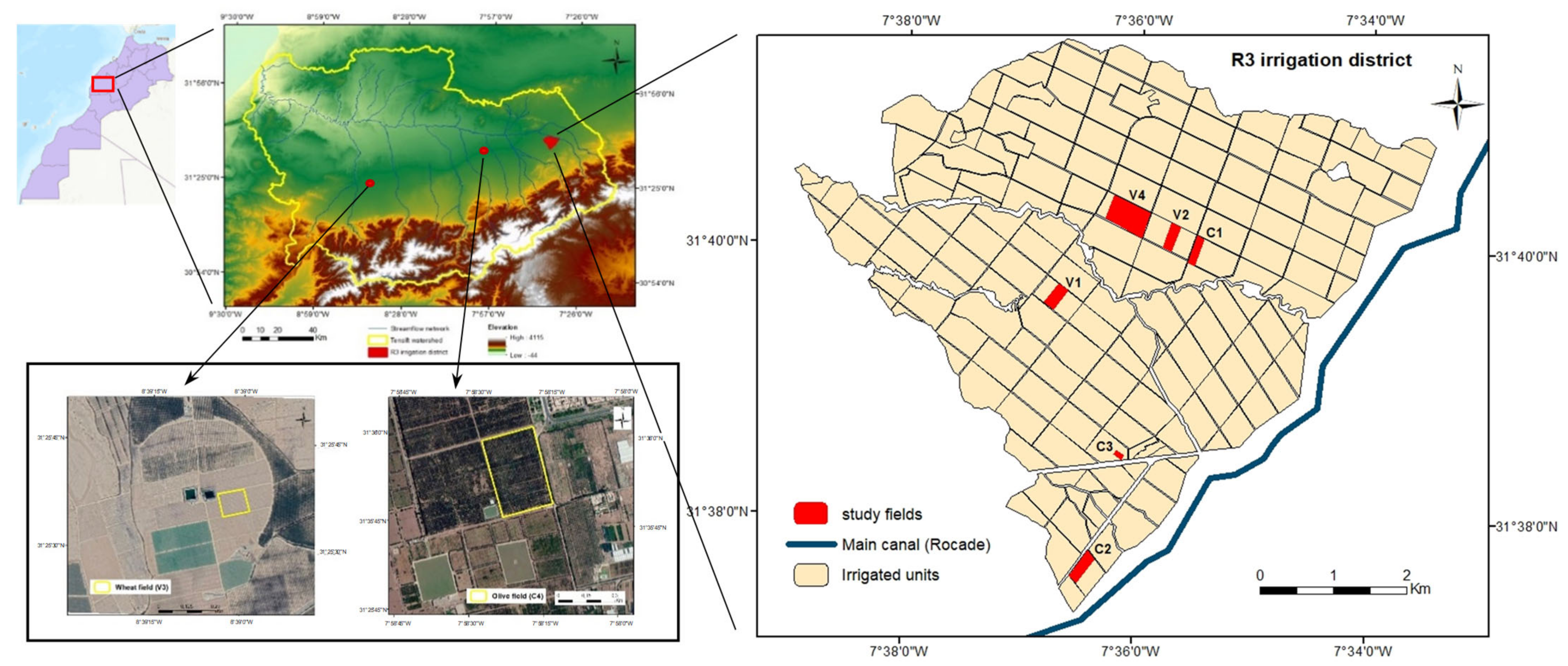
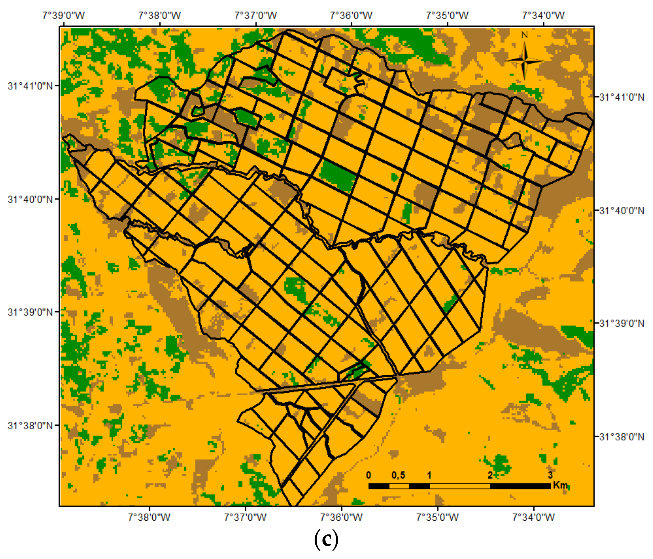
2.1. Study Area

The Haouz plain is located in central Morocco, around Marrakesh, to the north of the High Atlas mountain range. It lies between longitude 7°33′ to 7°39′ West and latitude 31°37′ to 31°42′ North, including approximately 3100 km² of irrigated area. The climate is Mediterranean semi-arid, with an average annual precipitation of about 250 mm, 70% of which falls during winter and spring, but it is characterized by a large inter- and intra-annual variability. The average air temperature ranges from 4 °C in winter to 37 °C in summer, with an average annual reference evapotranspiration of 1500 mm. The crops are irrigated using water from dams and river diversions from the high Atlas Mountains and water extracted from the underlying aquifer.

The irrigation schemes are fed by reservoirs, and water is diverted and distributed by gravity mainly through a hierarchic network of overhead concrete canals. Water delivery and the irrigation infrastructure for the whole irrigation system are managed by a water management agency called Office Régional de Mise en Valeur Agricole du Haouz (ORMVAH). The farmers are organized in Water User Associations (WUAs), which participate in the operation and maintenance of the irrigation system. Inside the tertiary unit, the water is rotated by the farmers themselves.

The area evaluated in this study (R3 irrigation district) during three seasons (2002–2003, 2005–2006 and 2008–2009) encompasses about 3000 ha of irrigated land (Figure 1), comprising about 745 individual plots, which became fully operative in 2000. There are three WUAs (Bni Krim, Od Garne and Argoub) operating in the R3 irrigation scheme with respective command areas of 600, 850 and 1550 ha that are supplied with water by 13, 20 and 35 tertiary canals respectively. The major crops in this area are cereals (mostly wheat) and olive trees, very often combined with an understory composed of weeds or wheat crop. The three studied agricultural seasons were contrasted in terms of climatic conditions, particularly the rainfall (P) and reference evapotranspiration (ETo) that influence the irrigation water requirement. The seasonal values from November to June for 2002–2003, 2005–2006 and 2008–2009 were respectively about 238 (with 108 mm falling in November), 218 and 274 mm for cumulative rainfall and about 726, 681 and 625 mm for total ETo.

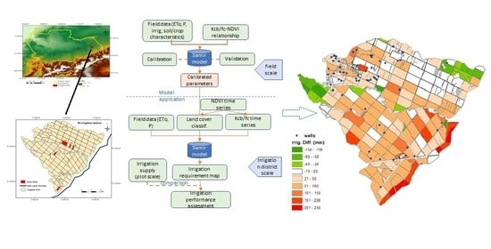
2.2. Model Description

The crop irrigation water requirements were simulated using a remote sensing-based soil water balance model that tracked daily changes in soil water storage as a function of inflows from effective rainfall and irrigation and outflows from deep percolation and actual evapotranspiration. The model was based on the well-known FAO56 dual crop coefficient approach [18], and we provide therefore in the following a brief description of the main calculations focusing on the modifications implemented in the SAMIR tool. The main originality of SAMIR lies in its use of a remote sensing NDVI time series for the monitoring of vegetation development from which crop coefficients and vegetation fraction covers are derived instead of using standard values.

The FAO56 approach is based on the concept of reference evapotranspiration for a standard, well-watered grass scaled by crop coefficients to account for the crop-specific development and influences on ET during a crop season. In the dual procedure, the crop coefficient is split into two components to account for the crop transpiration (basal crop coefficient, Kcb) and the evaporation from the soil (evaporation coefficient, Ke). Hence, the crop actual evapotranspiration is estimated as follows:

ET = (Ks∙Kcb + Ke)∙ETo

(1)

Ks is a stress coefficient which accounts for the reduction of transpiration due to decreasing water availability in the root zone. Daily reference evapotranspiration (ETo) is calculated using the FAO Penman—Monteith equation, given observations of daily maximum and minimum temperature, solar radiation, wind speed and vapor pressure.

The SAMIR tool performs a remote sensing-driven soil water balance based on the FAO56 dual crop method under non-standard conditions, i.e., considering the actual soil water status, as described in the FAO paper 56 [18] and summarized and extended in a subsequent paper [43]. Thus, NDVI time series [44] for vegetation monitoring are used to derive crop coefficients and fractional vegetation covers instead of the tabulated values. The NDVI, relying on near infra-red (NIR) and red (R) reflectances, is the most common vegetation index used to assess biophysical parameters and is available from most earth observation sensors [45].

$$NDVI=\frac{NIR-R}{NIR+R}$$

(2)

Discrete values of NDVI derived from satellite imagery are interpolated to daily time series and used to estimate the temporal evolution of biophysical components such as the basal crop coefficient (Kcb) and the fraction of soil surface covered by vegetation (fc) through linear NDVI–VIs relationships. The work of [20] constitutes a theoretical framework for these relationships, which is based on analytical relationships between LAI (Leaf Area Index) and the transpiration coefficient and between the LAI and multispectral VI. Several empirical relationships have been developed for different crops [19,20,21,22,23,29,46]. Regardless of the type of relationship, it depends on soil and vegetation properties and, as much as possible, should be calibrated to the study area concerned. If the area is sufficiently contrasted, the extreme values representing bare soil (NDVImin) and full cover (NDVImax) can be extracted from the image histogram [47]. Ref. [48] recommended the development and use of a linear relationship based on these extreme points for their ability to provide reliable estimates of water requirements when the demand is high at full cover.

In the case of soil evaporation, the model includes a modification to the calculation of the soil evaporation rate in the FAO approach. It consists of applying a correction coefficient (m) to the evaporation reduction coefficient (Kr) to prevent the rapid drying process of the soil surface by evaporation following the wetting events, simulated by the FAO-56 model under high evaporation conditions as reported by [49].

$$Kr=m·\frac{TEW-De}{TEW-REW}\le 1$$

(3)

where TEW represents the total evaporable water, REW the readily evaporable water and De the soil surface layer depletion in the shallow surface layer used to compute soil evaporation.

Following the FAO-56 model, soil evaporation is controlled by the soil surface layer depth (Ze), whereas crop transpiration is controlled by the root layer depth (Zr). In the SAMIR tool, a deep layer (Zd) was added below the root compartment to account for water storage and capillary rise [50]. To allow water stored in this deep layer to be used by the plant, a diffusion process was introduced to simulate capillary water movement between the deep layer and the root layer. For coherence, diffusion was also introduced between the root layer and the evaporation layer, especially to allow evaporation to decrease more slowly after a wetting event and to allow the deeper layers to continue drying after harvest. Lateral circulation of water (overland and subsurface runoff) is assumed to be negligible in the flat irrigated areas covered by this model. During rainfall or irrigation events, the water fills the compartments successively from top to bottom through gravity. When all the compartments are full, excess water flows out of the system through deep drainage (DP).

The root depth Zr varies according to the stage of plant development and is assumed to be linearly linked to the fractional vegetation cover (fc) according to Equation (4), which is analogous to Equation (8-1) in the FAO-56 paper [18], linking Zr to Kcb:

$$Zr=Zr\_min+\frac{fc}{fcmax}.\left(Zr\_max-Zr\_min\right)$$

(4)

where fcmax represents the maximum fraction cover corresponding to the maximum rooting depth (Zr_max) and Zr_min is the minimum rooting depth when the vegetation is detected by satellite (fc > 0). The critical water capacities of the evaporation and root layers (TEW, REW, TAW (total available water) and RAW (readily available water) following FAO-56 terminology) are computed as proposed in FAO-56 paper. Similarly, total available water in the deep compartment (TDW) is computed as:

$$TDW=\left(\theta fc-\theta wp\right)·Zd$$

(5)

where θfc and θwp are the volumetric water content at field capacity and wilting point, respectively.

Water diffusion due to capillary water movement, either upwards or downwards, is driven by the gradient between the water content of the two layers. The formalism is taken from [51] and is related to the difference in water content between the two layers as compared to field capacity. The diffusion between the surface and root layers (Dif_er) and between the root and deep layers (Dif_rd) is given by:

$$Di{f}_{er}=cd·\left(\frac{\frac{\left(TAW-Dr\right)}{Zr}-\frac{\left(TEW-De\right)}{Ze}}{\mathsf{\theta }fc}\right)$$

(6)

$$Di{f}_{rd}=cd·\left(\frac{\frac{\left(TDW-Dd\right)}{Zd}-\frac{\left(TAW-Dr\right)}{Zr}}{\mathsf{\theta }fc}\right)$$

(7)

where De, Dr and Dd represent depletion in the evaporation, root and deep layers, respectively, and cd is the diffusion coefficient (mm∙day⁻¹). The soil water balance is updated at a daily time step using the equations of the dual crop coefficient approach at the evaporation and root zone depths taking into consideration the water diffusion between layers and the deep layer defined above.

$$D{e}_j=0\le \left(D{e}_{j-1}+\frac{Ej}{few}+Tewj-Pj-\frac{Ij}{fw}-Di{f}_{er}\right)\le TEW$$

(8)

$$D{r}_j=0\le \left(D{r}_{j-1}-P_j-I_j+ET{c}_j-Di{f}_{rd}\right)\le TEW$$

(9)

$$D{d}_j=D{d}_{j-1}-DPr+Di{f}_{rd}\le TDW$$

(10)

where De_j, Dr_j and Dd_j are the depletions at the soil surface, root zone and deep layers at the end of day j (mm), P_j is the precipitation, I_j is irrigation depth, E_j is the soil evaporation, Tewj is the depth of transpiration from the exposed and wetted fraction of the soil surface layer, fw is the fraction of the soil surface wetted by irrigation and few is the wetted soil fraction exposed to evaporation.

In the SAMIR tool, the irrigation is triggered based on management rules set by the user and relies on the soil water status and the known or assumed farmer’s practices. The main parameters to be defined are the criteria for triggering irrigation, the irrigation depth and the soil fraction wetted by irrigation (fw). Different options are offered to trigger irrigation based on the level of RAW and the level of TAW on a given threshold of the root zone depletion (Dr) or at any fixed time step. In addition, in the case of annual crops which are not irrigated during senescence, irrigation will cease once the Kcb decreases below a given fraction of the peak value to be defined by the user. Additionally, other management rules can be used to further control the delivery of water at a seasonal scale, which are the maximum allowable cumulated water depth, the maximum number of irrigation events, a minimum and maximum application depth per event and a minimum interval between irrigation events.

2.3. Experimental Data

The soil water balance model was calibrated and validated using data sets collected during the SudMed project [52], which has been underway since 2001 in the Haouz semi-arid plain around Marrakesh (Morocco) and pursued in the frame of the Joint International Laboratory (Trema) [53].

Field experiments were conducted on six wheat fields during three growing seasons: three fields (C1, V1, V2) in 2002–2003 and two fields (C2, C3) in 2015–2016 located in the R3 district (35 km east of Marrakesh city, Morocco) and one field (V3) in 2016–017 located in the Mejjat region (70 km west of Marrakesh city). For olive trees, an experiment was carried out on an olive orchard (C4) located in the Agdal area (the southern boundary of Marrakesh city, Morocco) during the 2002–2003 season and another one (V4) in the R3 district during the 2005–2006 season. Five fields (C1, C2, C4, V1 and V2) were irrigated by flood system, and three fields (C3, V3 and V4) were supplied by drip irrigation system. The irrigation rates and frequencies differed among the fields and were more related to the surface irrigation scheduling in the R3 district in the case of the wheat fields and were more flexible for the other fields (wheat under drip irrigation and olive under both flood and drip irrigation) that relied on groundwater resources. The soil in the R3 district was clay loam, and its average water content at field capacity (θfc) and wilting point (θwp) used were the median values obtained by [54]. In the olive grove of the Agdal area, the soil was a silty clay loam, and average θfc and θwp used were median values derived from four pedotransfer functions [55,56,57,58]. In the wheat field (V3), the θfc and θwp used were derived from pedotransfer functions according to the soil texture of the field [59].

Flux measurement and meteorological stations were installed and allowed continuous monitoring of actual ET by an eddy covariance system (EC) and meteorological variables for ETo calculations. The meteorological measurements included incoming solar radiation (Kipp and Zonen CM5 Pyranometer, Delft, The Netherlands), air temperature and vapor pressure (HMP45C, Vaisala, Helsinki, Finland), wind speed (A100R Anemometer, R.M. Young Company, Traverse City, MI, USA) and rainfall (FSS500 Tipping Bucket Automatic Rain Gauge, Campbell Scientific Inc., Logan, UT, USA). The EC system consisted of a 3D sonic anemometer (CSAT3, Campbell Scientific Inc., Logan, UT, USA) and an open-path infrared gas analyzer (Li7500, 207 Licor Inc., Lincoln, NE, USA) or fast hygrometer (KH2O, Campbell Scientific Inc., Logan, UT, USA) that measured the fluctuations of the three components of wind speed, air temperature and water vapor. A complete description of the experiments can be found in [21,22] and [59] for wheat and in [60] and [61] for olive trees.

For the spatialized assessment of irrigation performance in the irrigation scheme using the remote sensing-based soil water balance model, irrigation volumes distributed in the R3 district were collected at the scale of the irrigated units (referred hereafter by the fields), which was the smallest unit for which water delivery was directly controlled by the Irrigation Department at ORMVAH. The water that is billed to farmers at the end of the season is delivered and measured at the tertiary canal intakes (serving the irrigated units) according to predefined water rates, and the water is then distributed to farmers inside the irrigated units by the Water Users Associations.

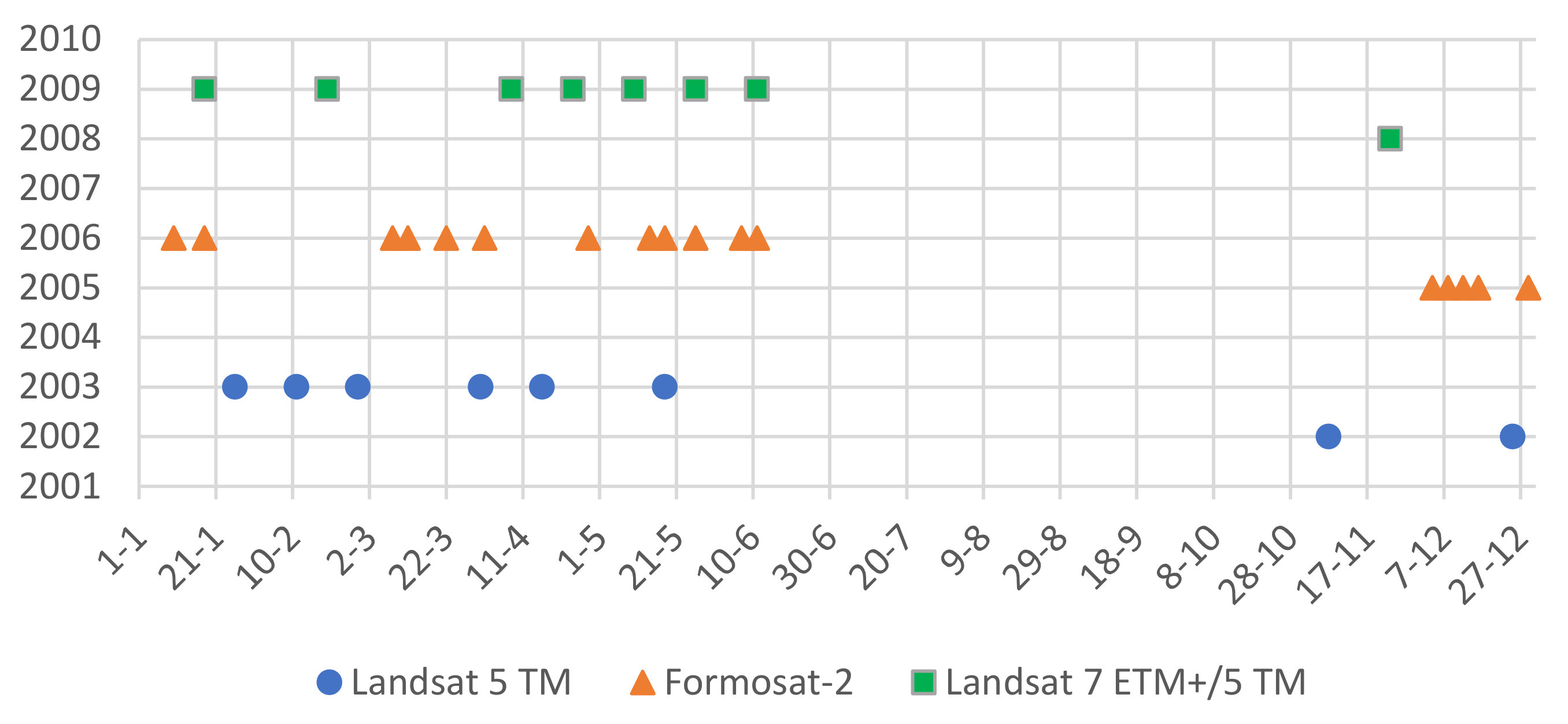
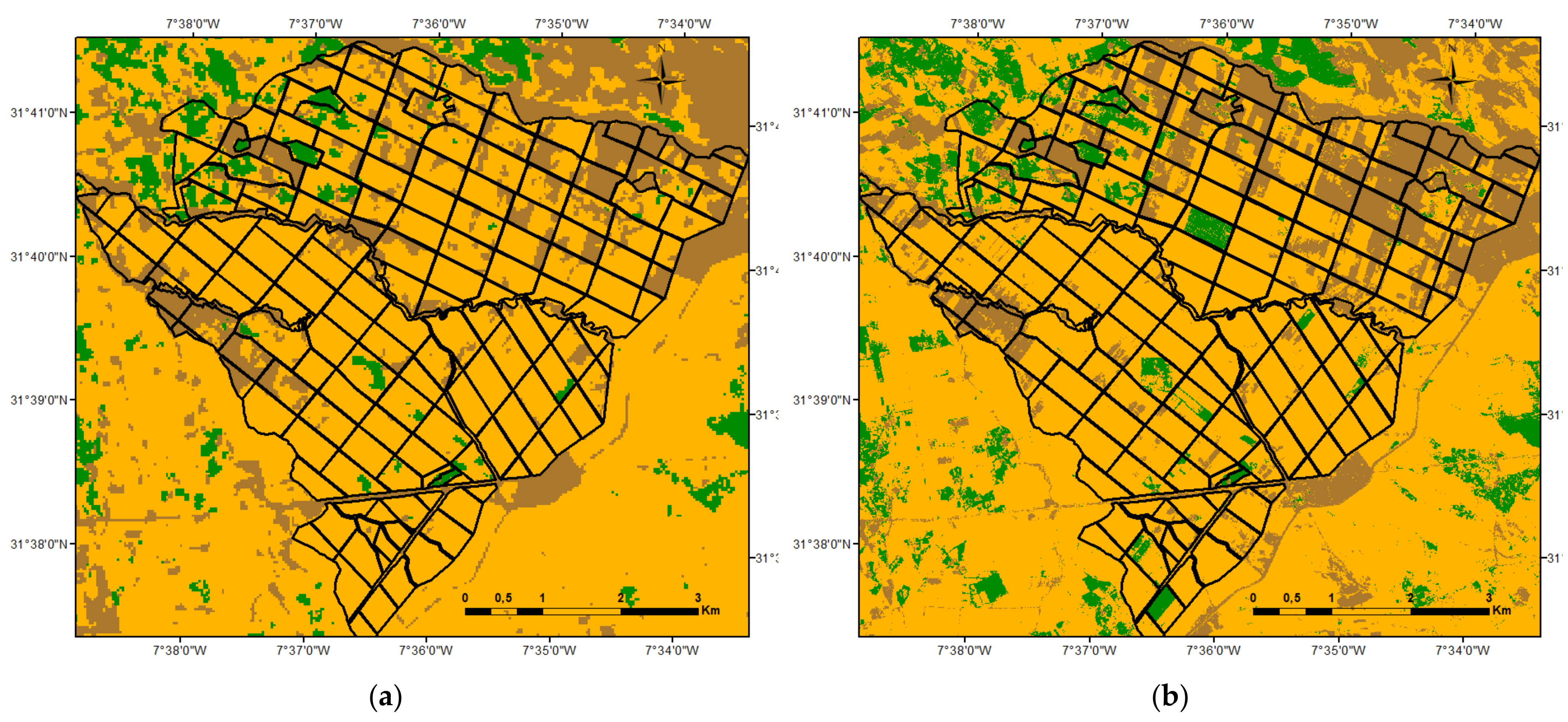
2.4. Satellite Data and Land Cover Mapping

A series of Landsat TM images of the studied area (Figure 2) acquired in 2002–2003 and 2008–2009 were geometrically and radiometrically corrected to provide a NDVI time series and a land cover map [62]. During the 2005–2006 season, a time series of FORMOSAT images was acquired over the R3 district and processed to produce a NDVI time series and a land cover map [63]. The NDVI profiles generated for each pixel were used to identify the main crop types of the study area using a decision-tree algorithm that was successfully applied in the region [62] and allowed the distinction of three broad land classes: bare soils/fallow, annual crops (mainly wheat) and trees (mainly olive trees) as presented in Figure 3. In fact, for simplification, we considered one single class for trees, grouping trees and trees with an understory (which could be either weeds or a wheat crop) which represented less than 10% of the R3 irrigation district area. The resulting land cover maps were evaluated using ground data, and the confusion matrix computed gave a global accuracy up to 80%, 85% and 76% respectively for the 2002–2003, 2005–2006 and 2008–2009 seasons (not shown here).

2.5. Model Calibration and Evaluation

The actual ET measured at the eight flux sites was used to calibrate and validate the model at plot scale. The model calibration procedure consisted of maximizing the Nash-Sutcliffe efficiency (NSE) criterion computed between observed and simulated ET using a steepest descent algorithm:

$$NSE=1-\frac{{\sum }_{i=1}^n(y_{iobs}-y_{isim}{)}^2}{{\sum }_{i=1}^n(y_{iobs}-\overline{y_{iobs}}{)}^2}$$

(11)

where n is the number of observations, $y_{isim }$ and $y_{iobs}$ are the values of simulated and observed variables for day i respectively and ${\overline{y}}_{iobs}$ is the average of observations over the study period.

In order to consider different climatic conditions and irrigation practices, the calibration was done using the data from the fields (C1, C2, C3) for wheat and the field C4 for olive trees, whereas the validation was achieved using the data from the fields (V1, V2, V3) for wheat and the field V4 for olive trees. The calibration was performed for the parameters controlling transpiration (Kcb, Zr_max, dif_dr, Z_tot (total soil depth)) and evaporation processes (dif_re, REW, Ze). Parameters based on ground observations were kept constant (NDVI-fc, θfc, θwp, init_RU (soil initial water content) and fw) as was the fraction of readily available water (p) specific to FAO-56 and for which little information was available. The Kcb and fc profiles were estimated from satellite data, and the other parameters, including Kcbmax (full cover), were calibrated based on ET measurements from the experimental sites. The calibrations were applied incrementally including parameters in the following order: first Zr_max controlling the plant available water, then parameters driving evaporation (REW, Ze and dif_er), then capillary rise (Z_tot and dif_rd) and finally Kcb. Observed irrigation values were used during this process, and the automatic irrigation mode was then switched on to calibrate irrigation parameters.

The performance of the results of the model calibration and validation was analyzed using three other statistical parameters: the correlation coefficient (R²) the root mean square error (RMSE) and the percent bias (PBIAS), which measured the correlation, the magnitude of the average error and the direction of the error bias between simulated and observed values, respectively:

$$RMSE=\sqrt{\frac{1}{n}\ast {\sum }_{i=1}^n(y_{isim}-y_{iobs}{)}^2}$$

(12)

$$R^2={\left[\frac{{\sum }_{i=1}^n\left(y_{isim}-\overline{y_{isim}}\right)\left(y_{iobs}-\overline{y_{iobs}}\right)}{{\sum }_{i=1}^n\left(y_{isim}-\overline{y_{isim}}\right){\sum }_{i=1}^n\left(y_{iobs}-\overline{y_{iobs}}\right)}\right]}^2$$

(13)

$$PBIAS=\left[\frac{{\sum }_{i=1}^n\left(y_{isim}-y_{iobs}\right)\ast 100}{{\sum }_{i=1}^n\left(y_{iobs}\right)}\right]$$

(14)

where ${\overline{y}}_{sim}$ and ${\overline{y}}_{obs}$ are the averages of simulated and observed values respectively.

After the calibration and validation process at plot scale, the model was used to estimate the spatially distributed irrigation water requirements at pixel scale over the R3 irrigation district, which were compared with the actual irrigation amounts supplied by ORMVAH during the 2002–2003, 2005–2006 and 2008–2009 seasons to evaluate irrigation performance.

3. Results

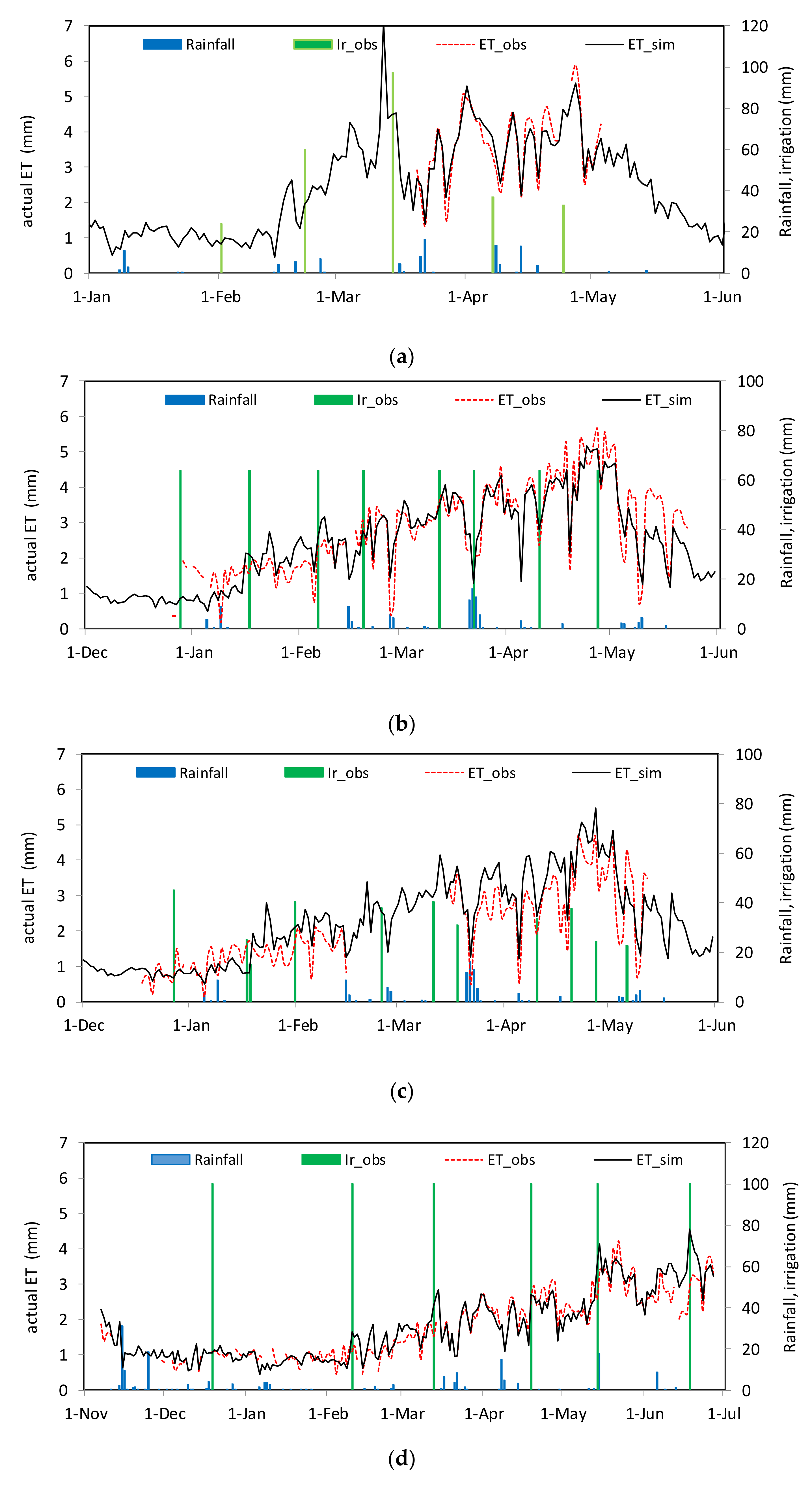
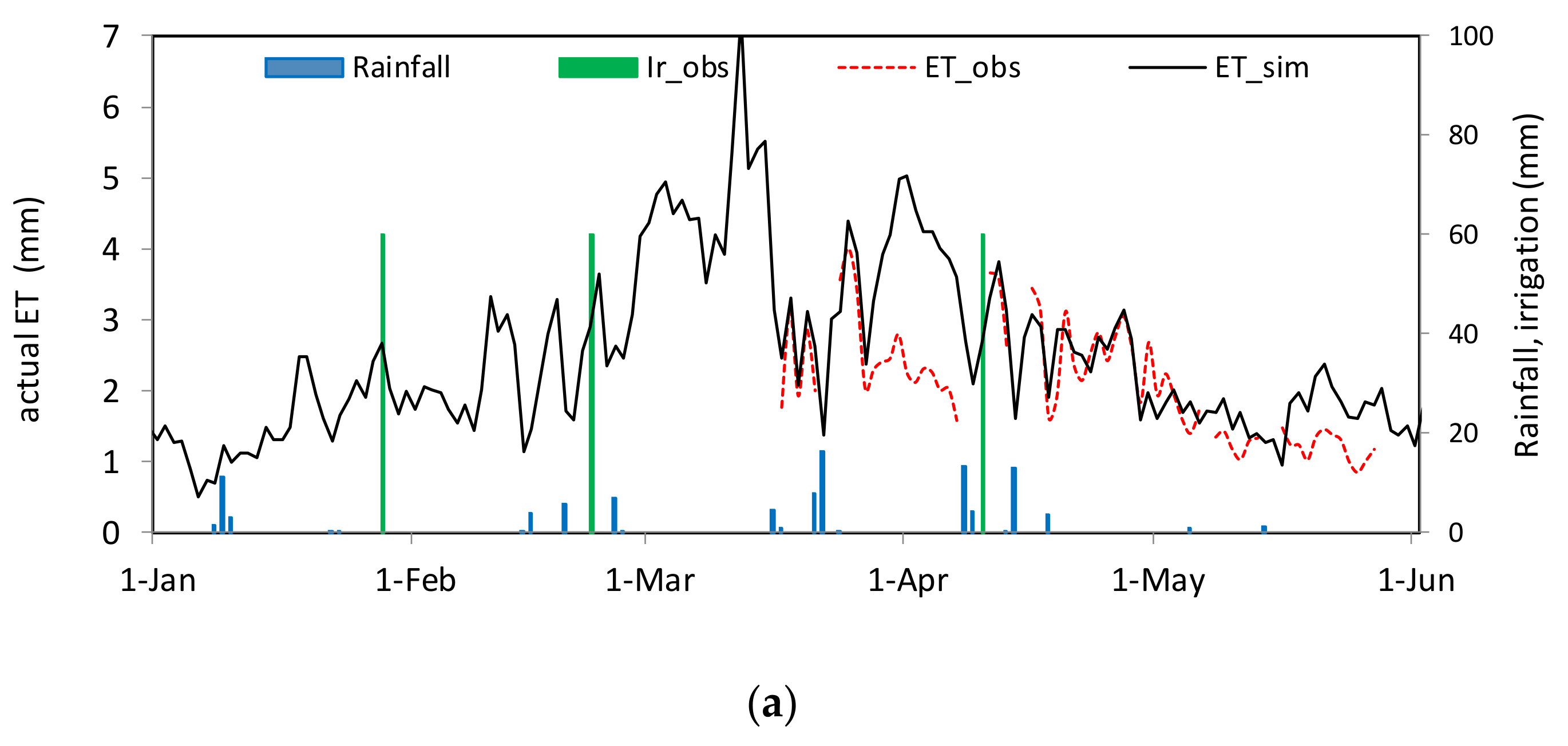
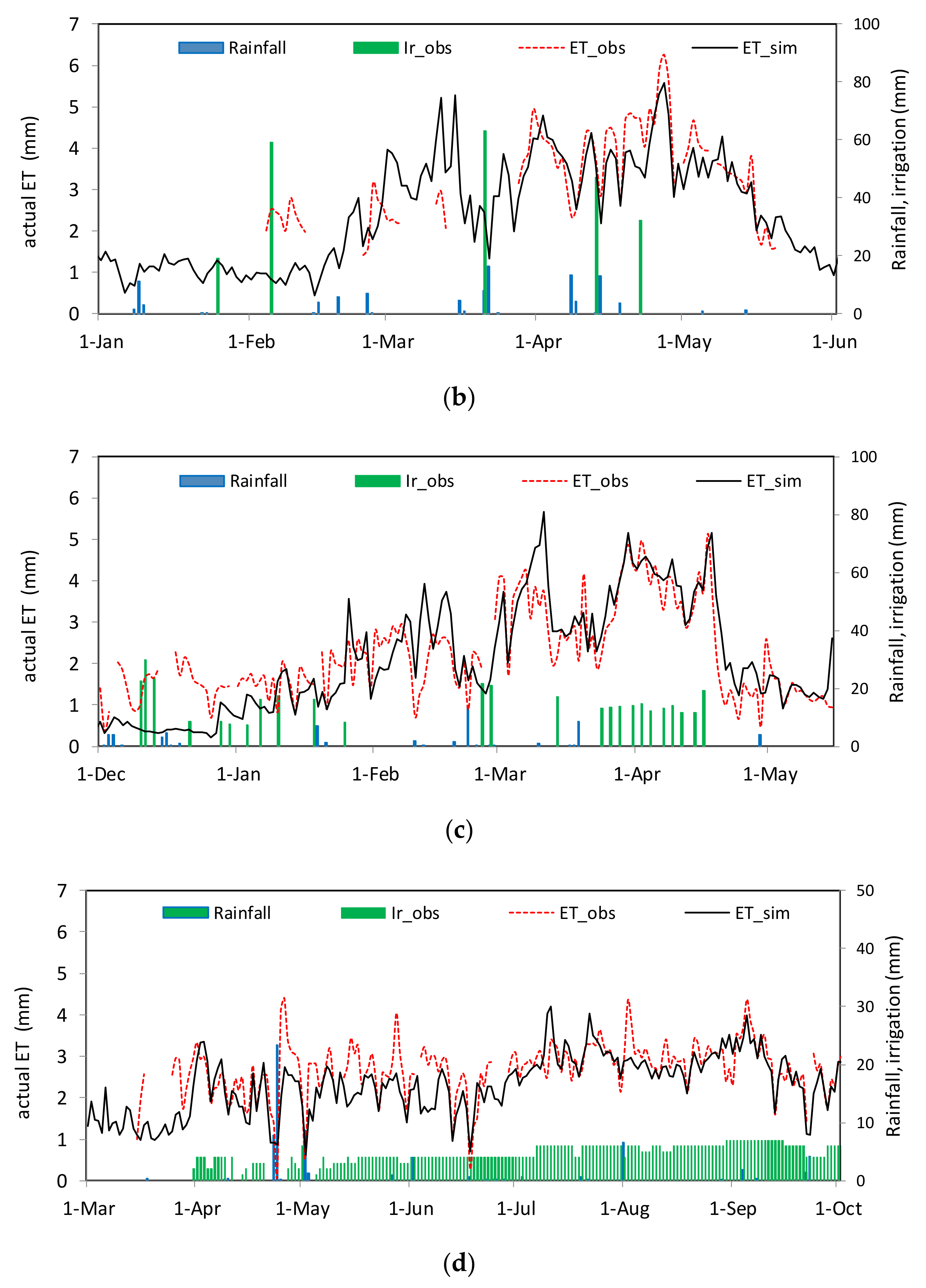
3.1. Calibration of the Model

The calibration was done for wheat simultaneously on three fields (C1 in 2002–2003 and C2 and C3 in 2015–2016) and for olive tree on the C4 field. The linear relations linking Kcb and fc with NDVI were established using values from the literature and NDVI values extracted from the image time series (

Table 1. Relations used for fractional vegetation cover (fc) and basal crop coefficient (Kcb) estimates from the Normalized Difference Vegetation Index (NDVI).

NDVI-fc	NDVI_min	NDVI_max	fc_min	fc_max	Relation	Sources
Wheat/olive tree	0.15	0.9	0	1	fc = 1.33*NDVI − 0.20	Min and Max NDVI taken in images assuming resp. bare soil and full cover
NDVI-Kcb	NDVI_min	NDVI_max	Kcb_min	Kcb_max	Relation	Sources
Wheat	0.15	0.9	0	1.05	Kcb = 1.40*NDVI − 0.21	Kcbmax calibrated
olive tree	0.15	0.9	0	0.76	Kcb = 1.01*NDVI − 0.15	Kcbmax calibrated

). For bare soil conditions, we assumed null values for Kcb and fc with the NDVI of bare soils extracted from the images, and at full cover (fc = 1), the corresponding NDVI was the maximum value extracted from the images [23,34,64]. The maximum Kcb values were calibrated for both wheat and olive tree (Table 1).

The daily Kcmax values were computed based on FAO-56 equation 72 using the measured meteorological data. The average value was 1.15, which was within the interval defined in FAO-56 ([1.05–1.3]) and was considered constant in the computation for simplification. A low initial water content of 10% was considered for the wheat plots because no significant rain was observed during the last days before the starting date of the simulation, whereas the olive grove had been irrigated four days previously and had a higher initial water content (init_RU = 0.8). The soil fraction wetted by rain or irrigation (fw) was set to one for the plots irrigated by flood technique, and it was set to 0.6 and 0.3, respectively, for the wheat plot and olive orchard using drip irrigation. The depth of the evaporation layer (Ze) and the proportion of easily available water (p) were set according to FAO paper 56 [18]. All other parameters were obtained by calibration (REW, m, Zr_max, Z_tot, Dif_er, Dif_rd) and are listed in

Table 2. Parameters obtained after calibration on observed crop evapotranspiration (ET) for wheat (three plots) and olive trees (one plot).

Parameter	Definition	Values				Data Source
		C1 (Wheat)	C2 (Wheat)	C3 (Wheat)	C4 (Olive)
	Soil Parameters:
θfc (m3/m3)	Volumetric water content at field capacity	0.35	0.35	0.35	0.36	ground observation
θwp (m3/m3)	Volumetric water content at wilting point	0.22	0.22	0.22	0.22	ground observation
Ze (mm)	Height of the soil evaporation layer	125	125	125	125	FAO56
REW	Readily evaporable water at surface layer	8	8	8	8	calibration
m	correction to the coefficient of evaporation reduction	0.58	0.58	0.58	0.28	calibration
Zr_min (mm)	Minimum root depth	125	125	125	125	FAO56
Zr_max (mm)	Maximum root depth	700	700	700	950	calibration
Z_tot (mm)	Total soil depth	1450	1450	1450	1450	calibration
p	fraction of TAW to be depleted before stress	0.55	0.55	0.55	0.65	FAO56
Difer	Diffusion between surface and root layers	16	16	16	0	calibration
Difrd	Diffusion between deep and root layers	8	8	8	7	calibration
Init_RU (%)	Soil initial water content	10	10	10	80	ground observation
	Irrigation Parameters:
fw	wetted fraction	1	1	0.6	1	ground observation
Kcb_off	Kcb threshold to stop irrigation (% of Kcbmax)	75	75	75	-	calibration
Ir_max (mm)	maximum irrigation rate	60	60	20	100	ground observation

.

Figure 4 shows the comparison between the measured and estimated actual evapotranspiration after the model calibration along with the amount of irrigation and rainfall over the three wheat fields (C1–C3) and the olive orchard (C4). For wheat, as mentioned previously, the calibration was performed jointly for the three fields by maximizing the average Nash criterion. The results showed that the ET estimated by the model was correctly adjusted to the measured ET. The average error statistics were about 0.84, 0.45 mm/day, 0.76 and 6% for NSE, RMSE, R² and Pbias, respectively, and they ranged from 0.75 to 0.89, 0.32 to 0.56 mm/day, 0.50 to 0.91 and −0.02 to 16% for NSE, RMSE and R², respectively. The detailed statistics are provided in

Table 3. Statistical values of the comparison between measured and modelled actual ET over the calibration and validation fields.

	Calibration Fields				Validation Fields
	C1	C2	C3	C4	V1	V2	V3	V4
NSE	0.89	0.86	0.75	0.82	0.66	0.76	0.59	0.62
RMSE (mm/day)	0.32	0.46	0.56	0.37	0.46	0.54	0.69	0.54
R2	0.91	0.86	0.50	0.86	0.67	0.83	0.80	0.67
Pbias (%)	0.2	0.02	16.5	4.2	−1.8	−9.9	0.8	−11.6

. It can be noted also that the temporal variations of simulated ET correctly follow the dynamic of the measured ET and are sensitive to the water supply events (irrigation and rainfall). These calibration results are improved compared to the local calibration performed over the same wheat field (C1) by [22,65] when using the standard FAO56 dual model and the Aquacrop model, respectively. For fields C2 and C3, the results are consistent (even improved for C2) with the validation undertaken by [66] when evaluating the performance of the Hydrus-1D model for ET estimation. However, an important overestimation of ET is observed during a period of high evaporation demand (25 March to 01 May) for the drip- irrigated field C3 (Pbias around 16%). This could be attributed to a reduction in soil evaporation and/or moderate water stress probably occurring during this period that was not accurately captured by the model (Ks was around 1.0), which reduced crop transpiration as a consequence to rapid soil drying in the limited fraction wetted by drip irrigation as reported by [66], particularly if the wetting events were not frequent enough to maintain adequate soil moisture, which was the case for field C3. Indeed, the drip irrigation system in this field was not adequately monitored (irrigation timing and rates not optimal) due to the lack of the farmer’s experience with this new technique. Additionally, during the late season, the model underestimated ET for both the C2 and C3 fields (after 07 May), which was probably caused by underestimation of soil evaporation, particularly after wetting events occurring at that end of the season. This may be explained by the reduction of the evaporation process in the soil surface, induced in the model by the value of the fraction cover (fc), which is kept constant and equal to its maximum (corresponding to NDVImax) until the end of the season. The discrepancies observed could also be attributed to the accuracy of the NDVI values derived from satellite images and the irrigation inputs recorded.

For olive trees, the calibration produced a good result because the dynamic of actual ET estimated by the model accurately followed the time course of observed actual ET (Figure 4d). The statistical values were 0.82, 0.37 mm/day, 0.86 and 4% for NSE, RMSE, R² and Pbias, respectively. Interestingly, the proposed model and the calibrated parameters values improved the ET estimates when compared with the results obtained on the same field by [61], with the standard FAO dualKc yielding RMSE and R² values of 0.54 mm/day and 0.58, respectively.

After calibration of the soil and vegetation parameters, irrigation was switched to automatic mode to calibrate related parameters based on a schedule that avoided stress (i.e., Dr values above the RAW) and with the irrigation rate corresponding to the water amount that will fill the depletion, limited by a maximum value Ir_max (mm) based on observed practices. Olive trees were irrigated all year round, whereas irrigation of wheat stopped at the beginning of the late period when Kcb decreased below a threshold kcb_off (corresponding to wheat drying before harvest) that needed calibration. For the wheat plots, the calibration consisted of minimizing both the difference between the total depths of the simulated irrigation and the observed one and the difference between the dates of the last simulated and observed irrigation events. The calibrated Kcb threshold to stop irrigation of wheat (Kcb_off = 75%) was consistent with the observed agricultural practices in the study area. Except for the C2 field, the simulated irrigation depths for C1 and C3 fields were similar to the observed ones (respectively 236, 320 mm and 251, 352 mm). For the C2 field, the total irrigation depth simulated by the model (359 mm) was 30% less than the observed one (512 mm), indicating applied irrigation higher than observed ET, which revealed an over-irrigation of this plot and that the amount in excess was probably lost by deep percolation. This difference could be attributed to the fact that, on one hand, this field received a high number of irrigation supplies (eight in total), all with a large rate (about 64 mm), and four of them were received during periods of low evaporation demand (between December and February), and on the other hand, some irrigation events coincided with rainfall (19 February, 22 March) which promoted the deep percolation losses. Regarding the date of the last irrigation supply for wheat, which was crucial for defining the Kcb_off parameter, the differences between the dates simulated and observed were quite low (−1, −3 and −4 days, respectively, for C1, C2 and C3).

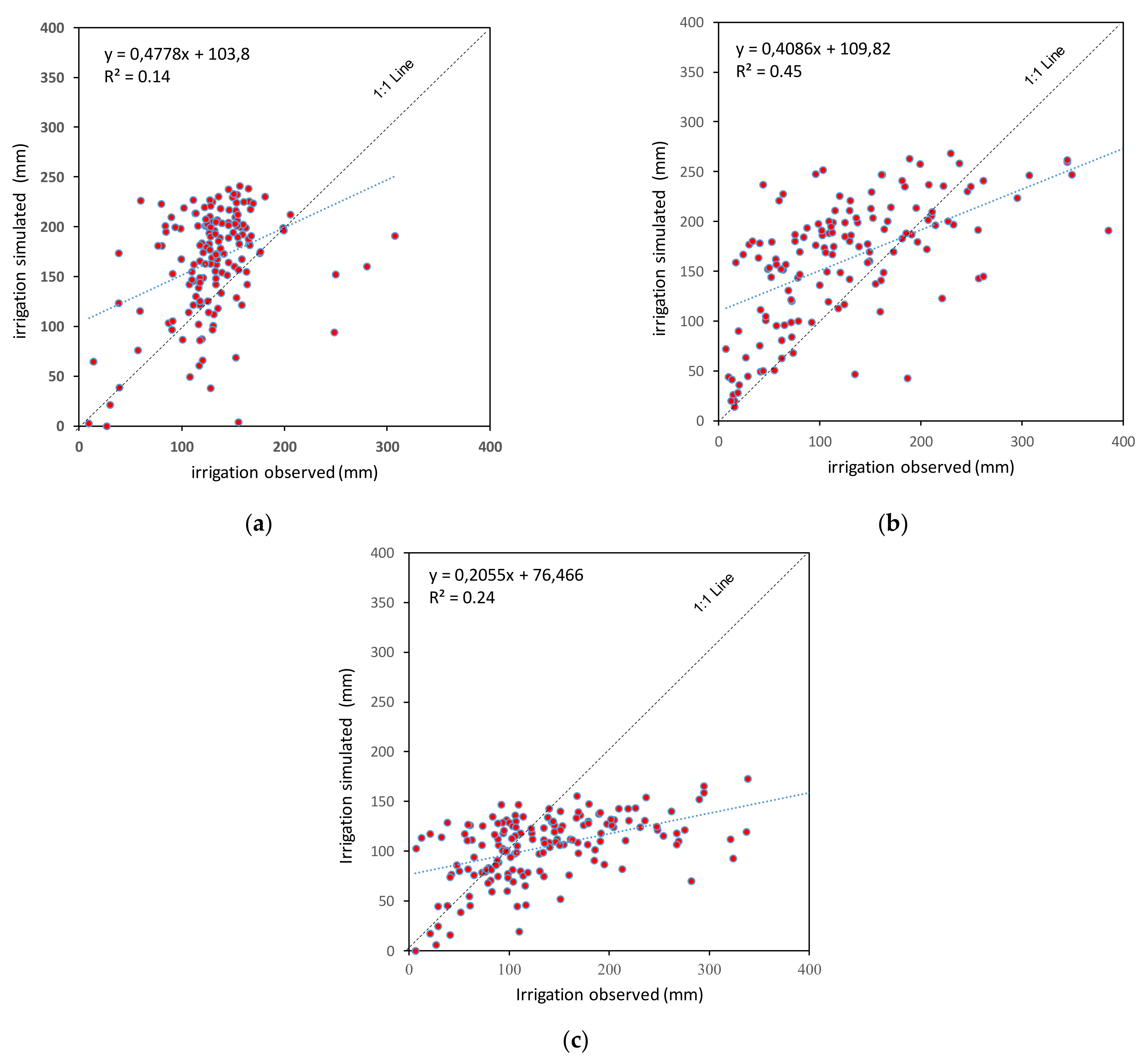
3.2. Validation of the Model

After calibration of the model, validation in terms of actual evapotranspiration estimates was performed using available measurements over the three wheat fields (V1, V2 in 2002–2003 and V3 in 2016–2017) and the olive field (V4 in 2005–2006). Figure 5 shows the comparison between the daily evolution of the simulated and observed actual ET along with the amount of irrigation and rainfall for the three wheat fields and the olive field. A general coherence is observed between the modeled and the measured ET across the growing season for all fields, suggesting a good performance of the model in estimating actual evapotranspiration. For wheat, the average NSE, RMSE, R² and Pbias values were 0.67, 0.56 mm/day, 0.77 and −4% ranging from 0.59 to 0.76, 0.46 to 0.69, 0.67 to 0.83 and −9.9% to 0.84% for C1, C2 and C3 fields, respectively. The detailed statistics are provided in Table 3. Interestingly, the actual ET estimated by the model was improved when compared both (i) to the local calibration of the standard FAO56 dual-Kc model performed over the same wheat fields (V1, V2) by [22], yielding NSE, RMSE and R² values of 0.17 (0.44), 0.99 (0.75) and 0.65 (0.76) for the V2 (V1) fields, respectively, and (ii) to the calibration of the Aquacrop model undertaken by [65], yielding NSE, RMSE and R² values of 0.05 (0.57), 1.07 (0.69) and 0.65 (0.85) for V2 (V1) fields, respectively. This could be explained by the introduction in the FAO56 model of diffusion between the root and evaporation layers (Diff_re) and the deep and root layers (Diff_rd), allowing evaporation to be fed through capillary rise particularly at the end of the cycle, and mitigating the occurrence of crop water stress through the contribution of the water stored in the deep layer to feed roots in dry conditions. For the V3 field irrigated by drip system, the results were slightly improved compared with the calibration of the standard FAO dualKc made on the same field by [59] yielding RMSE and R² values of 0.75 mm/day and 0.75, respectively. However, as noted by [59], an underestimation of the modelled ET during the initial stage is observed and is probably due to an underestimation of the soil evaporation, particularly when the irrigation events are more frequent, as with drip irrigation, which promotes more soil evaporation.

For olive trees, the validation was performed with the available data from an olive orchard in the R3 district irrigated by drip system. The NSE, RMSE, R² and Pbias were 0.62, 0.54 mm/day, 0.67 and −12%, respectively. This result showed that the daily simulated ET values agreed with the measured ET, and the dynamic of actual ET estimated by the model followed reasonably well the time course of observed actual ET (Figure 5d).

As in the calibration step, irrigation was switched to automatic mode using the irrigation parameters calibrated and the rules previously defined. For the wheat plots, except for the V1 field, the simulated irrigation depths for V2 and V3 fields were slightly close to the observed ones (respectively 230, 340 mm and 220, 374 mm). For the V1 field, the total irrigation depth simulated by the model (245 mm) was 36% higher than the irrigation applied (180 mm), which revealed an under-irrigation of this plot. In fact, according to the field survey, only three irrigation events had been scheduled during the whole growing season, and a great delay was observed between the second and the last event (about 47 days) which induced water stress and a decrease of observed ET (Figure 5a). Regarding the date of the last irrigation supply for wheat, the differences between the dates simulated and observed were −9, +3 and −1 days, respectively, for V1, V2 and V3. The last irrigation event was anticipated by the model for the V1 field (scheduled on 1 April, which coincided with a period of full wheat development under high evaporation demand) to avoid water stress that was observed as mentioned above. These results suggest that the Kcb threshold, defined as a percentage of the peak Kcb (full development), could be considered as a good proxy for the scheduling of the last irrigation for wheat, and the value obtained seemed to represent the farmers’ practices observed in the study areas.

Overall, the results obtained after calibration/validation processes show that the calibration performed provides an acceptable compromise for a set of calibrated parameters regardless of the irrigation system (flood or drip) when particularly used for evaluation of ET estimates over large areas without information on the irrigation system in place.

3.3. Model Application for Spatialized Estimates of RS-IWR

The model implemented in the SAMIR software was run over the whole R3 irrigated district using the image time series for the seasons 2002–2003, 2005–2006 and 2008–2009 and the calibrated parameters (Table 2). The soil in the district was considered almost homogeneous and we used the median values obtained by Boulet et al. (2009) for θfc and θwp. The initial soil water content (Init_RU) for annual crops was estimated considering previous precipitation and was set to 10% of the soil available water (between θfc and θwp) because no significant precipitation was observed before the starting dates of the simulation. For olive orchards, the initial soil water content was set to 50% because most of the olive farms had wells and were frequently irrigated regardless of surface water availability. Regarding irrigation rules, the minimal duration of the irrigation turns was set to 12 days according to local practices.

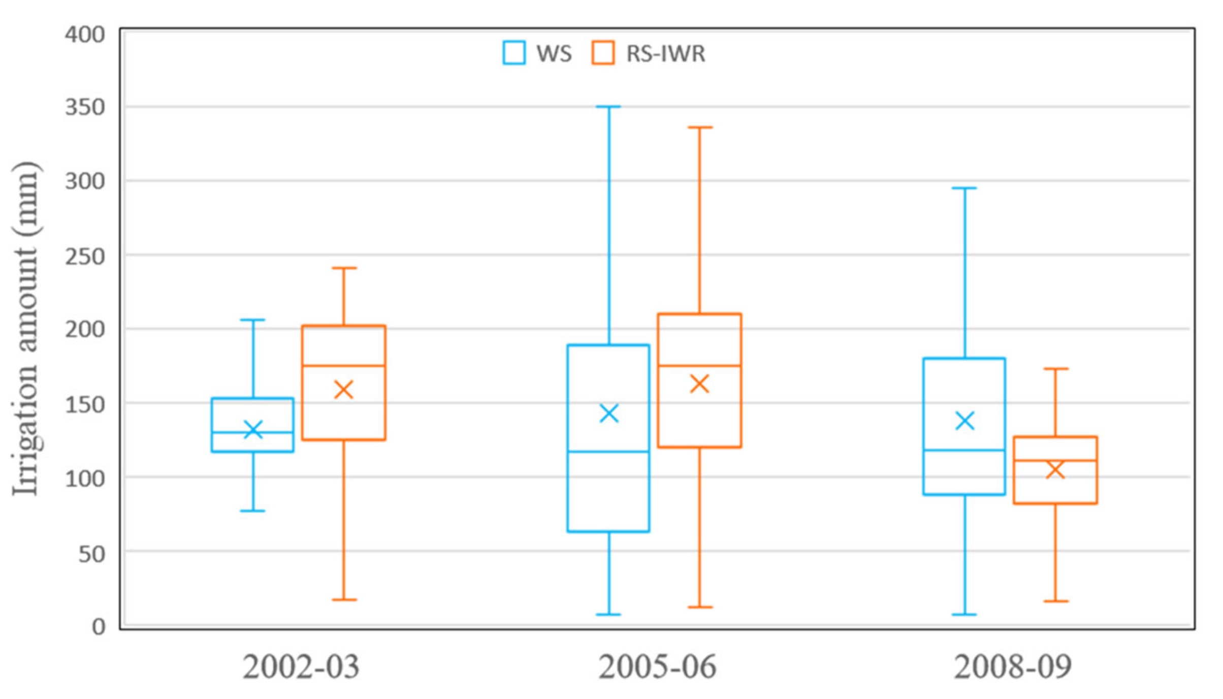
3.3.1. Analysis of Irrigation Water Practices

Figure 6 shows boxplots of the distribution of observed irrigation water supply (WS) and remotely sensed irrigation water requirements (RS-IWR) at field level during each of the three years of analysis. Clear shifts from one year to another can be observed both in the irrigation water applied and the irrigation water requirements. The median value of observed irrigation water was higher in 2002–2003 than in 2005–2006 and 2008–2009 (130, 117 and 118 mm respectively), but the shapes of the distribution were different. The dispersion of the WS values was significantly lower in 2002–2003, which was the driest year, than in the other seasons. This reveals that the irrigation water used by farmers varies considerably from year to year, which could be related to both farmers’ irrigation decision-making and delivery schedules made by the scheme managers that consider water availability and define water supply conditions. Regarding the modelled irrigation water requirements, median values were equal to about 175 mm in 2002–2003 and 2005–2006 and 112 mm in 2008–2009. Compared to observed water use, the dispersion of the RS-IWR values was lower in 2005–2006 and particularly in 2008–2009 (the wettest year), in which a large part of the crop water requirements were covered by the rainfall, but it was higher in 2002–2003 (the driest year). This suggests that even in water shortage conditions, the crop development was not spatially homogeneous, and some farmers have made better use of limited water (deficit irrigation) along with adequate agricultural practices to ensure acceptable crop growth, a fact that will be evident in the sections below. The overall difference between the distributions of observed water use and modelled water requirements showed that the sensitivity to variation in weather conditions was smaller for the observed water use. This apparent lack of sensitivity suggests that factors other than weather conditions could explain the farmers’ individual irrigation behavior.

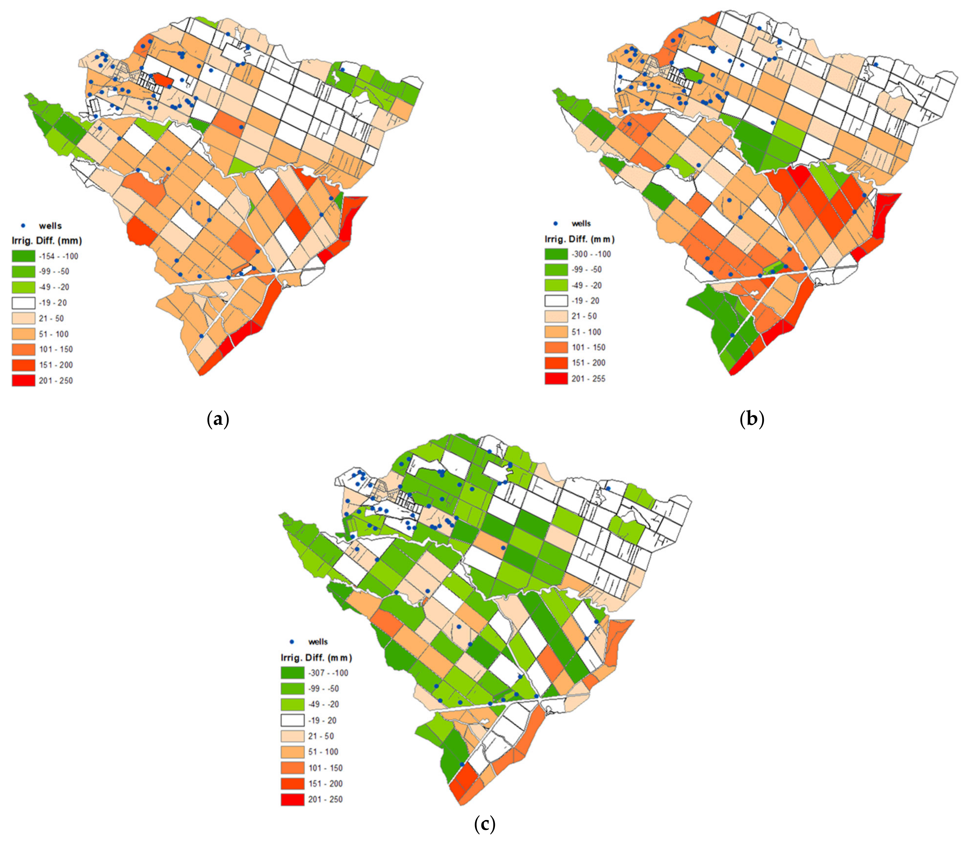
3.3.2. Comparison of Irrigation Water Use Anomalies

To evaluate field-level irrigation water use within the irrigation district, we compared the annual irrigation water supplied with the corresponding modelled irrigation water requirement for each field in the area during the three seasons (Figure 7). The figure shows differences in the scatterplots across the three seasons and a great variability between fields for each season. No strong correlation was found between the observed irrigation water applied and the irrigation requirement (R² was equal to 0.14, 0.44 and 0.24 for 2002–2003, 2005–2006 and 2008–2009, respectively), which revealed an inconsistency in irrigation water use across fields in the district. The dotted lines in Figure 7 represent the perfect correspondence between water requirements and water supplied. Most of the fields fell above the 1:1 line in 2002–2003 and 2005–2006, knowing that these years were characterized by high climatic demand (Section 2.1), which showed that the farmers irrigated below the estimated irrigation water requirements of the crops. In addition, the field points (Figure 7) in 2002–2003 (the driest season) were less scattered than in 2005–2006, which means that the water supplied in that year was more homogeneous across fields as previously shown (Figure 6). Indeed, during this season with insufficient rainfall and higher climatic demand, the farmers relied critically on irrigation supplies for their crops that were restricted by the scheme managers due to decreased water availability in the dam. In 2008–2009, the majority of the fields fell below the 1:1 line, indicating that those fields were over-irrigated even if the abundant rainfall was able to cover a large amount of crop water requirements, which revealed the inadequacy of the irrigation scheduling.

The analysis of the distribution over the three years of the “water use anomaly” indicator, which is calculated as the difference between the applied irrigation water and the remote sensing estimates of irrigation water requirements at field level [67], shows large variability across the three seasons. In 2002–2003, primarily negative water use anomalies are observed, indicating that most of the fields (>75%) experienced water stress conditions, homogeneously receiving water amounts below the irrigation requirements within the district (anomalies concentrated around the median value of −24%). In 2005–2006, even if the irrigation supply was not restricted and the season was rainy, the irrigation water use pattern was surprisingly heterogeneous, with over 75% of the fields under-irrigated and a larger magnitude of anomalies. Conversely, there was a major shift in 2008–2009 (the wettest year) toward positive water use anomalies (>62% of the fields) reflecting apparent irrigation supplies above water demands. Hence, we could hypothesize that in irrigation management, both the farmers and the scheme managers fail to adequately consider the magnitude of interannual changes in irrigation requirements induced by weather conditions, which could be attributed partly to the lack of reliable spatial information on the current soil water status.

Figure 8 presents the spatial distribution of the difference between the remote sensing estimates of the irrigation water requirements and the applied irrigation water at field level over the irrigation scheme for the three seasons. The spatial representation of the water use anomalies over the irrigation scheme allows visual inspection of the irrigation water use pattern, which enables the identification of areas with irrigation problems which could help managers assess irrigation performance in addition to controlling illicit use of irrigation water. Particularly, some fields identified as under-irrigated could have benefitted from groundwater extractions, as is apparent through the spatial distribution of those fields, which are located close to the wells (Figure 8a,b). However, this valuable information could likely be obtained in seasons experiencing water shortage conditions (either reduced rainfall or surface water supply restrictions) and/or seasons suffering inadequate irrigation scheduling. Other examples concern the identification of: (i) areas located along the southeast boundary of the perimeter (in red on the map) that officially received no water but probably pumped it directly from the main channel which passes along their southern boundary or (ii) the areas located at both the northeast and southeast boundaries (in green on the map) for which water use largely exceeds water requirements, suggesting that this excess of water supplied was probably used for areas outside the district boundaries, which is illegal. The irrigation practices, which could explain the spatial variability observed, may be influenced by various factors including biophysical drivers (e.g., weather, crop, soil characteristics, etc.), socio-economic conditions and other behavioral considerations. Thus, an investigation needs to be undertaken in the studied area in order to identify and better understand the drivers of the actual farmers’ decision making.

The discrepancies identified between the field-level irrigation water supplies and the remote-sensed estimates of the irrigation requirements may be attributed to uncertainties in irrigation water records or model estimates. In fact, during every irrigation turn, the managers deliver the water until the tertiary canal intakes according to predefined water rates, and the water is then distributed to farmers inside the tertiary units by the Water Users Associations. In some cases, the water could be reallocated for different reasons, either to other fields due to agreements arranged between farmers or to fields owned by the same farmer, particularly at the tertiary canal level, resulting in some fields receiving more water than the amount allocated whereas others received less [68]. On the other hand, the errors in the modelled irrigation water needs could result from the assumption made for a homogeneous soil type in the irrigation district, knowing that soil properties account among the key parameters for irrigation water requirement estimates. The same result was reported by [69] when using the same approach, applying an RS-based soil water balance model to estimate irrigation water requirements over a large irrigation area in the southeast of Spain. The model errors could also be attributed to the simplifications adopted to describe the soil water dynamics and crop development, whereas these processes are more complex to represent both in time and space [13]. While these errors cannot be ignored, regarding the good validation results of the actual evapotranspiration obtained in the studied region, the variability observed in the irrigation water use still relies on differences in farmer’s agricultural practices, including irrigation, and scheme manager strategies for irrigation water management as previously reported in the region [21,68]. Interestingly, the approach proposed allows to detect this variability and provides interesting insights into spatial and temporal irrigation water use patterns, which enables identifying possible factors that could explain irrigation behaviors [67].

4. Conclusions

Evaluating the spatial and temporal distribution of the crop irrigation water requirement at field level using remote sensing-based soil water balance models provides interesting insights regarding irrigation water use when compared with in-situ monitoring of observed irrigation water supplied at the irrigation district scale.

The evaluation at plot scale of the remote sensing-based FAO56 soil water balance model implemented in the SAMIR software, under different weather and water management conditions, provided acceptable estimates of actual ET, indicated by low values of RMSE obtained for wheat (0.56 mm/day) and olive trees (0.54 mm/day), which were the main crops in the region. The model also showed its ability to provide good estimates of irrigation water requirements and could be applied for evaluating irrigation water use in large-scale irrigated areas.

The results of the model application over an irrigation scheme in the Haouz plain (central Morocco) for estimating spatially distributed irrigation water requirements showed a clear spatial variability in irrigation water use between fields, and particularly that the observed water use decisions were less sensitive to interannual variability of weather conditions than modelled irrigation water requirements. It could be inferred that in irrigation management, both the farmers and the scheme managers fail to adequately consider the magnitude of interannual changes in irrigation requirements induced by weather conditions, which could be attributed partly to a lack of reliable spatial information on the current soil water status. In addition to the model and the observed data uncertainties, the variability observed could be attributed to different other factors including: (i) the irrigation supply conditions that depend on water availability and inadequate irrigation scheduling by the scheme managers and (ii) the farmer’s socio-economic considerations and management practices (cultivar, sowing date, irrigation, fertilizers, weed control, etc.).

Importantly, this study demonstrates the opportunity to combine in-situ monitoring information with a remote sensing-based soil water balance model for assessing field-level irrigation decision-making in order to improve irrigation performance. The irrigation managers would likely appreciate using operational tools based on the approach presented in this study, which could allow for a reliable assessment of irrigation delivery performance at the scale of irrigation schemes and provide an enhanced irrigation advisory service by delivering customized and near real-time information on crop development status and irrigation needs to farmers or Water Users Associations. These tools enable the improvement of irrigation scheduling for efficient and profitable agricultural water management, particularly in water limited areas.

References

1. FAO. AQUASTAT Database. 2016. Available online: http://www.fao.org/nr/water/aquastat/data (accessed on 3 November 2020).
2. UN Water. Integrated Monitoring Guide for SDG 6: Targets and Global Indicators; UN Water: Geneva, Switzerland, 2016. [Google Scholar]
3. Bastiaanssen, W.G.M.; Brito, R.A.L.; Bos, M.G.; Souza, R.A.; Cavalcanti, E.B.; Bakker, M.M. Low cost satellite data for monthly irrigation performance monitoring: Benchmarks from Nilo Coelho, Brazil. Irrig. Drain. Syst. 2001, 15, 53–79. [Google Scholar] [CrossRef] [Green Version]
4. Lorite, I.J.; Mateos, L.; Fereres, E. Evaluating Irrigation Performance in a Mediterranean Environment: II. Variability among Crops and Farmers. Irrig. Sci. 2004, 23, 85–92. [Google Scholar] [CrossRef]
5. Santos, C.; Lorite, I.J.; Allen, R.G.; Fereres., E. Performance Assessment of an Irrigation Scheme Using Indicators Determined with Remote Sensing Techniques. Irrig. Sci. 2010, 28, 461–477. [Google Scholar] [CrossRef] [Green Version]
6. Taghvaeian, S.; Neale, C.M.U.; Osterberg, J.C.; Sritharan, S.I.; Watts, D.R. Remote Sensing and GIS Techniques for Assessing Irrigation Performance: Case Study in Southern California. J. Irrig. Drain. Eng. 2018, 144, 2–10. [Google Scholar] [CrossRef]
7. Rana, G.; Katerji, N. Measurement and estimation of actual evapotranspiration in the field under Mediterranean climate: A review. Eur. J. Agron. 2000, 13, 125–153. [Google Scholar] [CrossRef]
8. Allen, R.G.; Pereira, L.S.; Howell, T.A.; Jensen, M.E. Evapotranspiration information reporting: I. Factors governing measurement accuracy. Agric. Water Manag. 2011, 98, 899–920. [Google Scholar] [CrossRef] [Green Version]
9. Blatchford, M.L.; Mannaerts, C.M.; Zeng, Y.; Nouri, H.; Karimi, P. Status of accuracy in remotely sensed and in-situ agricultural water productivity estimates: A review. Remote Sens. Environ. 2019, 234, 111413. [Google Scholar] [CrossRef]
10. Tasumi, M.; Allen, R.G. Satellite-based ET mapping to assess variation in ET with timing of crop development. Agric. Water Manag. 2007, 88, 54–62. [Google Scholar] [CrossRef]
11. Gowda, P.; Chavez, J.; Colaizzi, P.; Evett, S.; Howell, T.; Tolk, J. ET mapping for agricultural water management: Present status and challenges. Irrig. Sci. 2008, 26, 223–237. [Google Scholar] [CrossRef] [Green Version]
12. Karimi, P.; Bastiaanssen, W.G.M. Spatial evapotranspiration, rainfall and land use data in water accounting—part 1: Review of the accuracy of the remote sensing data. Hydrol. Earth Syst. Sci. 2015, 19, 507–532. [Google Scholar] [CrossRef] [Green Version]
13. Calera, A.; Campos, I.; Osann, A.; D’Urso, G.; Menenti, M. Remote sensing for crop water management: From ET modelling to services for the end users. Sensors 2017, 17, 1104. [Google Scholar] [CrossRef] [Green Version]
14. Norman, J.M.; Kustas, W.P.; Humes, K.S. Source approach for estimating soil and vegetation energy fluxes in observations of directional radiometric surface temperature. Agric. For. Meteorol. 1995, 77, 263–293. [Google Scholar] [CrossRef]
15. Bastiaanssen, W.G.M.; Menenti, M.; Feddes, R.A.; Holtslag, A.A.M. A remote sensing surface energy balance algorithm for land (SEBAL). 1. Formulation. J. Hydrol. 1998, 212–213, 198–212. [Google Scholar] [CrossRef]
16. Allen, R.G.; Tasumi, M.; Morse, A.; Trezza, R.; Wright, J.L.; Bastiaanssen, W.; Kramber, W.; Lorite, I.J.; Robison, C.W. Journal of Irrigation and Drainage Engineering Satellite-Based Energy Balance for Mapping Evapotranspiration with Internalized Calibration (METRIC)—Applications. J. Irrig. Drain. Eng. 2007, 133, 395–406. [Google Scholar] [CrossRef]
17. Jensen, M.E.; Wright, J.L.; Pratt, B.J. Estimating Soil Moisture Depletion from Climate, Crop and Soil Data. Trans. ASAE 1971, 14, 954–959. [Google Scholar] [CrossRef]
18. Allen, R.G.; Pereira, L.S.; Raes, D.; Smith, M. Crop evapotranspiration: Guidelines for computing crop requirements. In Irrigation and Drainage Paper No. 56; FAO: Rome, Italy, 1998; p. 300. [Google Scholar]
19. Bausch, W.C.; Neale, C.M.U. Crop coefficients derived from reflected canopy radiation-a concept. Trans. ASABE 1987, 30, 703–709. [Google Scholar] [CrossRef]
20. Choudhury, B.J.; Ahmed, N.U.; Idso, S.B.; Reginato, R.J.; Daughtry, C.S.T. Relations between evaporation coefficients and vegetation indices studied by model simulations. Remote Sens. Environ. 1994, 50, 1–17. [Google Scholar] [CrossRef]
21. Duchemin, B.; Hadria, R.; Erraki, S.; Boulet, G.; Maisongrande, P.; Chehbouni, A.; Escadafal, R.; Ezzahar, J.; Hoedjes, J.C.B.; Kharrou, M.H.; et al. Monitoring wheat phenology and irrigation in Central Morocco: On the use of relationships between evapotranspiration, crops coefficients, leaf area index and remotely-sensed vegetation indices. Agric. Water Manag. 2006, 79, 1–27. [Google Scholar] [CrossRef]
22. Er-Raki, S.; Chehbouni, A.; Guemouria, N.; Duchemin, B.; Ezzahar, J.; Hadria, R. Combining FAO56 model and ground-based remote sensing to estimate water consumptions of wheat crops in a semi-arid region. Agric. Water Manag. 2007, 87, 41–54. [Google Scholar] [CrossRef] [Green Version]
23. González-Dugo, M.P.; Mateos, L. Spectral vegetation indices for benchmarking water productivity of irrigated cotton and sugar beet crops. Agric. Water Manag. 2008, 95, 48–58. [Google Scholar] [CrossRef]
24. Campos, I.; Neale, C.M.U.; Calera, A.; Balbontín, C.; González-Piqueras, J. Assessing satellite-based basal crop coefficients for irrigated grapes (Vitis vinifera L.). Agric. Water Manag. 2010, 98, 45–54. [Google Scholar] [CrossRef]
25. Er-Raki, S.; Rodriguez, J.C.; Garatuza-Payan, J.; Watts, C.J.; Chehbouni, A. Determination of crop evapotranspiration of table grapes in a semi-arid region of Northwest Mexico using multi-spectral vegetation index. Agric. Water Manag. 2013, 122, 12–19. [Google Scholar] [CrossRef]
26. Odi-Lara, M.; Campos, I.; Neale, M.C.; Ortega-Farías, S.; Poblete-Echeverría, C.; Balbontín, C.; Calera, A. Estimating evapotranspiration of an apple orchard using a remote sensing-based soil water balance. Remote Sens. 2016, 8, 253. [Google Scholar] [CrossRef] [Green Version]
27. Diarra, A.; Jarlan, L.; Er-Raki, S.; Le Page, M.; Aouade, G.; Tavernier, A.; Boulet, G.; Ezzahar, J.; Merlin, O.; Khabba, S. Performance of the two-source energy budget (TSEB) model for the monitoring of evapotranspiration over irrigated annual crops in North Africa. Agric. Water Manag. 2017, 193, 71–88. [Google Scholar] [CrossRef]
28. Glenn, E.P.; Neale, C.M.U.; Hunsaker, D.J.; Nagler, P.L. Vegetation index-based crop coefficients to estimate evapotranspiration by remote sensing in agricultural and natural ecosystems. Hydrol. Process. 2011, 25, 4050–4062. [Google Scholar] [CrossRef]
29. Hunsaker, D.J.; Pinter, P.J., Jr.; Barnes, E.M.; Kimball, B.A. Estimating cotton evapotranspiration crop coefficients with a multispectral vegetation index. Irrig. Sci. 2003, 22, 95–104. [Google Scholar] [CrossRef]
30. Nagler, P.; Scott, R.; Westenberg, C.; Cleverly, J.; Glenn, E.; Huete, A. Evapotranspiration on western U.S. rivers estimated using the Enhanced Vegetation Index from MODIS and data from eddy covariance and Bowen ratio flux towers. Remote Sens. Environ. 2005, 97, 337–351. [Google Scholar] [CrossRef]
31. Katul, G.; Schieldge, J.; Hsieh, C.I. Skin temperature perturbations induced by surface layer turbulence above a grass surface. Water Resour. Res. 1998, 34, 1265–1274. [Google Scholar] [CrossRef]
32. Campos, I.; Villodre, J.; Carrara, A.; Calera, A. Remote sensing-based soil water balance to estimate Mediterranean holm oak savanna (dehesa) evapotranspiration under water stress conditions. J. Hydrol. 2013, 494, 1–9. [Google Scholar] [CrossRef]
33. Mateos, L.; González-Dugo, M.P.; Testi, L.; Villalobos, F.J. Monitoring evapotranspiration of irrigated crops using crop coefficients derived from time series of satellite images. I. Method validation. Agric. Water Manag. 2013, 125, 81–91. [Google Scholar] [CrossRef]
34. Pôças, I.; Paço, T.; Paredes, P.; Cunha, M.; Pereira, L.S. Estimation of actual crop coefficients using remotely sensed vegetation indices and soil water balance modelled data. Remote Sens. 2015, 7, 2373–2400. [Google Scholar] [CrossRef] [Green Version]
35. Cherif, R.; Simonneaux, V.; Rivalland, V.; Gascoin, S.; Le Page, M.; Ceschia, E. Distributed Modelling of Evapotranspiration Using High-Resolution NDVI maps Over Cropland in South-west France; General Assembly 2012, Vienna. 14.1061C; European Geosciences Union (EGU): Munich, Germany, 2012. [Google Scholar]
36. Le Page, M.; Simonneaux, V.; Thomas, S.; Metral, J.; Duchemin, B.; Kharrou, H.; Cherkaoui, M.; Chehbouni, A. SAMIR A Tool for Irrigation Monitoring Using Remote Sensing for Evapotranspiration Estimate. In Technological Perspectives for Rational Use of Water Resources in the Mediterranean Region; El Moujabber, M., Mandi, L., Trisorio-Liuzzi, G., Martín, I., Rabi, A., Rodríguez, R., Eds.; CIHEAM: Bari, Italy, 2009; pp. 275–282. Available online: http://om.ciheam.org/om/pdf/a88/00801202.pdf (accessed on 13 February 2021).
37. Melton, F.S.; Johnson, L.F.; Lund, C.P.; Pierce, L.L.; Michaelis, A.R.; Hiatt, S.H.; Guzman, A.; Adhikari, D.; Purdy, A.J.; Rosevelt, C.; et al. Satellite irrigation management support with the terrestrial observation and prediction system: A framework for integration of satellite and surface observations to support improvements in agricultural water resource management. IEEE J. Sel. Top. Appl. Earth Obs. Remote. Sens. 2012, 5, 1709–1721. [Google Scholar] [CrossRef]
38. González-Dugo, M.P.; Escuin, S.; Cano, F.; Cifuentes, V.; Padilla, F.L.M.; Tirado, J.L.; Oyonarte, N.; Fernández, P.; Mateos, L. Monitoring evapotranspiration of irrigated crops using crop coefficients derived from time series of satellite images. II. Application on basin scale. Agric. Water Manag. 2013, 125, 92–104. [Google Scholar] [CrossRef]
39. Vuolo, F.; D’Urso, G.; De Michele, C.; Bianchi, B.; Cutting, M. Satellite-based irrigation advisory services: A common tool for different experiences from Europe to Australia. Agric. Water Manag. 2015, 147, 82–95. [Google Scholar] [CrossRef]
40. Calera Belmonte, A.; Jochum, A.M.; García Cuesta, A.; Rodríguez Montoro, A.; Fuster López, P. Irrigation management from space: Towards user-friendly products. Irrig. Drain. Syst. 2005, 19, 337–353. [Google Scholar] [CrossRef]
41. Moreno, R.; Arias, E.; Sánchez, J.L.; Cazorla, D.; Garrido, J.; Gonzalez-Piqueras, J. HidroMORE2: An optimized and parallel version of HidroMORE. In Proceedings of the 8th International Conference on Information and Communication Systems (ICICS), Irbid, Jordan, 4–6 April 2017; pp. 1–6. [Google Scholar]
42. Simonneaux, V.; Le Page, M.; Helson, D.; Metral, J.; Thomas, S.; Duchemin, B.; Cherkaoui, M.; Kharrou, H.; Berjami, B.; Chehbouni, G. Estimation spatialisée de l’évapotranspiration des cultures irriguées par télédétection: Application à la gestion de l’irrigation dans la plaine du Haouz (Marrakesh, Maroc). Sécheresse 2009, 20, 123–130. [Google Scholar] [CrossRef] [Green Version]
43. Allen, R.G.; Pereira, L.S.; Smith, M.; Raes, D.; Wright, J.L. FAO-56 dual crop coefficient method for estimating evaporation from soil and application extensions. J. Irrig. Drain. Eng. ASCE 2005, 131, 2–13. [Google Scholar] [CrossRef] [Green Version]
44. Rouse, J.W.; Haas, R.H.; Schell, J.A.; Deering, D.W.; Harlan, J.C. Monitoring the Vernal Advancement and Retrogradation of Natural Vegetation; NASA/GSFC, Type III, Final Report; NASA: Greenbelt, MD, USA, 1974; pp. 1–371. [Google Scholar]
45. Pôças, I.; Calera, A.; Campos, I.; Cunha, M. Remote sensing for estimating and mapping single and basal crop coefficients: A review on spectral vegetation indices approaches. Agric. Water Manag. 2020, 233. [Google Scholar] [CrossRef]
46. Campos, I.; Neale, C.M.U.; López, M.-L.; Balbontín, C.; Calera, A. Analyzing the effect of shadow on the relationship between ground cover and vegetation indices by using spectral mixture and radiative transfer models. J. Appl. Remote Sens. 2014, 8, 083562. [Google Scholar] [CrossRef]
47. Gutman, G.; Ignatov, A. The derivation of the green vegetation fraction from NOAA/AVHRR data for use in numerical weather prediction models. Int. J. Remote Sens. 1998, 19, 1533–1543. [Google Scholar] [CrossRef]
48. Campos, I.; Neale, C.; Suyker, A.; Arkebauer, T.; Gonçalves, I. Reflectance-based crop coefficients redux: For operational evapotranspiration estimates in the age of high producing hybrid varieties. Agric. Water Manag. 2017, 187, 140–153. [Google Scholar] [CrossRef] [Green Version]
49. Torres, E.A.; Calera, A. Bare soil evaporation under high evaporation demand: A proposed modification to the fao-56 model. Hydrol. Sci. J. 2010, 55, 303–315. [Google Scholar] [CrossRef]
50. Zhang, Y.; Wegehenkel, M. Integration of MODIS data into a simple model for the spatial distributed simulation of soil water content and evapotranspiration. Remote Sens. Environ. 2006, 104, 393–408. [Google Scholar] [CrossRef]
51. Devonec, E.; Barros, A.P. Exploring the transferability of a land-surface hydrology mode. J. Hydrol. 2002, 265, 258–282. [Google Scholar] [CrossRef]
52. Chehbouni, A.; Escadafal, R.; Duchemin, B.; Boulet, G.; Simonneaux, V.; Dedieu, G.; Mougenot, B.; Khabba, S.; Kharrou, H.; Maisongrande, P.; et al. An Integrated Modelling and Remote Sensing Approach for Hydrological Study in Arid and Semi-arid Regions: The SUDMED Programme. Int. J. Remote Sens. 2008, 29, 5161–5181. [Google Scholar] [CrossRef] [Green Version]
53. Jarlan, L.; Khabba, S.; Er-Raki, S.; Le Page, M.; Hanich, L. Remote Sensing of Water Resources in Semi-Arid Mediterranean Areas: The joint international laboratory TREMA. Int. J. Remote Sens. 2015, 36, 4879–4917. [Google Scholar] [CrossRef]
54. Boulet, G.; Mougenot, B.; Ben Abdelouahab, T. An evaporation test based on Thermal InfraRed remote-sensing to select appropriate soil hydraulic properties. J. Hydrol 2009, 376, 589–598. [Google Scholar] [CrossRef] [Green Version]
55. Wösten, J.H.M. Pedotransfer functions to evaluate soil quality. In Soil Quality for Crop Production and Ecosystem Health; Developments in Soils Science; Gegorich, E.G., Carter, M.R., Eds.; Elsevier: Amsterdam, The Netherlands, 1997; Volume 25, pp. 221–245. [Google Scholar]
56. Wösten, J.H.M.; Lilly, A.; Nemes, A.; Le Bas, C. Development and use of a database of hydraulic properties of European soils. Geoderma 1999, 90, 169–185. [Google Scholar] [CrossRef]
57. Saxton, K.E.; Rawls, W.J.; Romberger, J.S.; Papendick, R.I. Estimating generalized soil-water characteristics from texture. Soil Sci. Soc. Am. J. 1986, 50, 1031–1036. [Google Scholar] [CrossRef]
58. Campbell, C.S. Soil Physics with Basic; Elsevier: New York, NY, USA, 1985; p. 149. [Google Scholar]
59. Rafi, Z.; Merlin, O.; Le Dantec, V.; Khabba, S.; Mordelet, P.; Er-Raki, S.; Amazirh, A.; Olivera-Guerra, L.; Ait Hssaine, B.; Simonneaux, V.; et al. Partitioning evapotranspiration of a drip-irrigated wheat crop: Inter-comparing eddy covariance-, sap flow-, lysimeter- and FAO-based methods. Agric. For. Meteorol. 2019, 265, 310–326. [Google Scholar] [CrossRef]
60. Ezzahar, J.; Chehbouni, A.; Hoedjes, J.C.B.; Er-Raki, S.; Chehbouni, A.; Boulet, G.; Bonnefond, J.M.; De Bruin, H.A.R. The use of the scintillation technique for monitoring seasonal water consumption of olive orchards in a semi-arid region. Agric. Water Manag. 2007, 89, 173–184. [Google Scholar] [CrossRef] [Green Version]
61. Er-Raki, S.; Chehbouni, A.; Boulet, G.; Williams, D.G. Using the dual approach of FAO56 for partitioning ET into soil and plant components for olive orchards in a semiarid region. Agric. Water Manag. 2010, 97, 1769–1778. [Google Scholar] [CrossRef] [Green Version]
62. Simonneaux, V.; Duchemin, B.; Helson, D.; Er-Raki, S.; Olioso, A.; Chehbouni, A.G. The use of high-resolution image time series for crop classiication and evapotranspiration estimate over an irrigated area in central Morocco. Int. J. Remote Sens. 2008, 29, 95–116. [Google Scholar] [CrossRef] [Green Version]
63. Duchemin, B.; Hagolle, O.; Mougenot, B.; Benhadj, I.; Hadria, R.; Simonneaux, V.; Ezzahar, J.; Hoedjes, J.; Khabba, S.; Kharrou, M.H.; et al. Agrometeorological study of semi-arid areas: An experiment for analysing the potential of time series of FORMOSAT-2 images (Tensift-Marrakesh plain). Int. J. Remote Sens. 2008, 29, 5291–5299. [Google Scholar] [CrossRef] [Green Version]
64. Carpintero, E.; Mateos, L.; Andreu, A.; González-Dugo, M.P. Effect of the differences in spectral response of Mediterranean tree canopies on the estimation of evapotranspiration using vegetation index-based crop coefficients. Agri. Water Manag. 2020, 238. [Google Scholar] [CrossRef]
65. Toumi, J.; Er-Raki, S.; Ezzahar, J.; Khabba, S.; Jarlan, L.; Chehbouni, A. Performance assessment of AquaCrop model for estimating evapotranspiration, soil water content and grain yield of winter wheat in Tensift Al Haouz (Morocco): Application for irrigation management. Agric. Water Manag. 2016, 163, 219–235. [Google Scholar] [CrossRef]
66. Er-Raki, S.; Ezzahar, J.; Merlin, O.; Amazirh, A.; Ait Hssaine, B.; Kharrou, M.H.; Khabba, S.; Chehbouni, A. Performance of the HYDRUS-1D model for water balance components assessment of irrigated winter wheat under different water managements in semi-arid region of Morocco. Agric. Water Manag. 2021, 244, 106546. [Google Scholar] [CrossRef]
67. Foster, T.; Goncalves, I.Z.; Campos, I.; Neale, C.M.U.; Brozovic, N. Assessing landscape scale heterogeneity in irrigation water use with remote sensing and in-situ monitoring. Environ. Res. Lett. 2019, 14, 024004. [Google Scholar] [CrossRef]
68. Kharrou, M.H.; Le Page, M.; Chehbouni, A.; Simonneaux, V.; ErRaki, S.; Simonneaux, V. Assessment of equity and adequacy of water delivery in irrigation systems using remote sensing-based indicators in semi-arid region, Morocco. Water Resour. Manag. 2013, 27, 4697–4714. [Google Scholar] [CrossRef]
69. Garrido-Rubio, J.; González-Piqueras, J.; Campos, I.; Osann, A.; González-Gómez, L.; Calera, A. Remote sensing–based soil water balance for irrigation water accounting at plot and water user association management scale. Agric. Water Manag. 2020, 238, 106236. [Google Scholar] [CrossRef]
Figure 1. Map of the study area. Upper left panel: Location of the study area in the Tensift watershed (Morocco); Right panel: R3 irrigation district and location of six experimental fields (C1, C2, C3, V1, V2, V4); Lower left panel: Location of two other experimental fields (V3, C4).
Remotesensing 13 01133 g001
Figure 2. Acquisition dates for the satellite images during the three growing seasons.
Remotesensing 13 01133 g002
Figure 3. Land cover maps for the 2002–2003 (a), 2005–2006 (b) and 2008–2009 (c) seasons in the R3 irrigation district. The colors represent the trees (in green), the wheat crop (in yellow) and bare soil/fallow (in brown).
Remotesensing 13 01133 g003aRemotesensing 13 01133 g003b
Figure 4. Comparison between measured and simulated actual ET after model calibration over three wheat fields: C1 (a) in 2002–2003, C2 (b) and C3 (c) in 2015–2016 and the olive trees C4 (d) in 2002–2003.
Remotesensing 13 01133 g004
Figure 5. Comparison between measured and simulated actual ET over the validation fields: three wheat fields V1 (a) and V2 (b) in 2002–2003, V3 (c) in 2016–2017), and the olive tree V4 (d) in 2005–2006.
Remotesensing 13 01133 g005aRemotesensing 13 01133 g005b
Figure 6. Distribution of observed irrigation water use (WS) and remotely sensed irrigation water requirements (RS-IWR) at field level for the three seasons.
Remotesensing 13 01133 g006
Figure 7. Comparison between observed irrigation supply and modeled irrigation water requirements at field level in the three seasons (a) 2002, (b) 2005–2006 and (c) 2008–2009.
Remotesensing 13 01133 g007
Figure 8. Map of differences between modeled irrigation requirements and observed irrigation water at field scale in the R3 irrigation district over the seasons 2002–2003 (a), 2005–2006 (b) and 2008–2009 (c).
Remotesensing 13 01133 g008