1. Introduction
Pavement maintenance procedures and measures are important to ensure safe and unobstructed traffic flow and to maintain pavement condition-prescribed engineering and operational values. Maintenance procedures and measures should be based on data on the actual condition of the pavement and its physical properties. These data are traditionally collected through digging test-pits and by extracting cores [
1]. These methods cannot provide a complete picture of pavement conditions because the data are related to a specific location. In addition, these methods are destructive because they require disruption of traffic and repair of a pavement section. Therefore, data about the pavement condition are very often obtained by nondestructive testing (NDT) methods, such as pavement deflection testing [
2], laser scanning [
3], infrared thermography (IRT) [
4] and ground-penetrating radar (GPR) [
5,
6]. According to [
7], the data collected with GPR are essential for the pavement rehabilitation project.
The GPR method is based on the emission of low power electromagnetic waves to obtain images of the subsurface layers [
6]. The reflection and scattering of wide-band electromagnetic waves transmitted by radar occur as a result of discontinuities in the electrical and magnetic properties of the studied structure. The echoes detected in the examined structures or subsurface layers are then converted into images using signal processing and imaging techniques.
The application of GPR as an effective tool for subsurface inspection of transportation infrastructure is constantly evolving. It is used to determine the location of reinforcements [
8], the condition of pipes [
9], the degree of compaction of the asphalt layer [
10], and delamination between asphalt layers [
11], as well as to detect moisture damage in the asphalt pavement [
12]. However, GPR has been the most widely used method for determining the pavement layer thickness, which was its primary function [
5,
13]. Pavement layer thickness provides very important information for determining bearing capacity, estimating remaining pavement life, strengthening planning of existing pavement and quality control during and after construction. From the beginning of its application, GPR has shown a high degree of accuracy in estimating asphalt layer thickness.
In the following sections, studies on the accuracy of determining asphalt layer thickness using GPR with air-coupled antennas are presented. For newly constructed pavements with asphalt layer thicknesses of 100 to 250 mm, [
14] showed a thickness error of 2.9%. In the 2000s, the accuracy of GPR measurements was systematically researched in the USA [
15,
16,
17]. According to a test conducted in Virginia [
15], an HMA layer thickness error of about 3% was found when the individual layers were resolved in the reflected GPR signal. The error increased to 12% when the entire HMA layer was considered without resolving the thin layers. In accordance with [
16], conducted on heavily trafficked highways in Virginia, the error in determining asphalt layer thickness ranged from 3.7% to 8.4%, with a mean of 5.7%. The GPR error in determining asphalt layer thickness ranged from 3.7% to 11.8%, with a mean of 8.0%, as reported by [
17]. Analysis of the GPR data collected from different sites showed that thickness error increases with pavement age—4.4% error for 0- to 5-year-old pavements and 5.8% error for pavements older than 20 years having surfaces older than 10 years [
14]. In Croatia, studies have been conducted on motorways, regional and county roads and on runways [
18,
19]. The error for new pavements of motorways was mostly less than 10% and varied from 0.16% to 12.32% [
18]. For regional and county roads that have been in service for years, the error ranges from 6.70% to 14.83% [
18]. The thickness of asphalt overlays on runways was found to have a relative error ranging from 1.7% to 10.3% [
19].
The repeatability of GPR measurements has also been investigated. In [
20], where three sets of data were collected at the same locations and at different time periods, thickness errors ranging from 5.9% to 12% were found. The discrepancy in the results can be explained by changes in the value of the dielectric constant due to the different moisture content of the test location, and same day measurements showed good repeatability. The speed of the survey had no significant effect on the performance of the GPR [
17]. It was found that the thickness error was 6.7% for steady state measurements, 7.9% for low speed and 8.3% for high speed measurements [
17]. Thus, GPR is capable of acquiring data at speeds up to 100 km/h [
21].
Although GPR applications on airfields are similar to those on road pavements, less research has been conducted on airfields. GPR has been successfully applied to determine the thicknesses of all runway pavement layers [
19]. According to [
22], GPR and infrared thermography are two nondestructive testing (NDT) methods that are efficient in airfield inspection. Infrared thermography was used to locate cracks and other anomalies and GPR was used to determine the depth and thickness of these defects. Testing GPR along with other NDT methods to detect voids under airfield pavements showed that the advantage of GPR is that it can quickly process a large amount of data [
23]. GPR has been successfully used at airfields in Poland to determine the direction of cracks and structural voids and to detect dowels and anchors in concrete slabs [
24].
3D GPR is a useful tool for airfields, as it allows fast and economical surveying of the large areas of runways and taxiways [
25]. As stated by [
26], 3D GPR mapping and imaging is an efficient tool for airfield inspection and construction planning.
The data obtained by a GPR measurement only provides information about the thickness of asphalt layers in the longitudinal survey lines compared to the 3D GPR. GPR data are sufficient for the rehabilitation planning of road pavements, but not for airfield pavements. Airfield pavements are much wider than roads and have many sections with different construction histories and thus different pavement structures. To deal with this problem, a method to create a spatial representation (3D model) based on the GPR data was presented [
27]. The main disadvantage of this method is that it is time consuming, requiring a large number of survey lines and additional processing of the GPR data. This disadvantage is especially a problem at airports where measurements must be made with traffic at short intervals. However, the value of the collected and interpreted data overcomes the above disadvantage.
The aim of this study is to investigate the influence of different distances between survey lines on the accuracy of 3D models of asphalt layer thickness.
2. Materials and Methods
The research was conducted on the apron of Pula airport in Croatia. The apron area is approximately 60,000 m
2. The structure of the apron pavement consists of asphalt layers placed on an unbound base course. Some sections of the apron have asphalt layers that are more than 30 years old—i.e., well beyond their expected service life (
Figure 1). The pavement had many cracks propagating in various directions, both longitudinally and transversely, as well as radially in all directions.
Research procedure consisted of the following steps:
2.1. GPR Data Collection
The GPR system shown in
Figure 2 was used to collect the data on the total asphalt layer thickness of the apron pavement. The system consists of two air-coupled antennas (1.0 and 2.0 GHz), a central unit for connecting the system components (SIR 20), a computer for processing and storing the data and a Distance Measuring Instrument (DMI). The system is supplemented by a high resolution digital camera. Antennas with 1.0 and 2.0 GHz central frequencies offer a very good compromise between the possible depth and the recording resolution for determining the pavement thickness; the transmitters and receivers are located in each antenna. They are separated by a duplexer that allows each antenna to transmit and receive electromagnetic waves (monostatic type of radar).
Before starting data collection, certain parameters and filters need to be set (
Table 1). Position correction is the parameter that controls the length of the time that the system will acquire data. Range gain controls the time-variable gain. Gain is signal amplification used to compensate for the natural effects of signal attenuation. As the transmitted signal passes through a material, it will attenuate as the material absorbs some signal. Gain amplifies that signal after it is received to compensate for signal losses and make weaker reflectors easier to see. A Finite impulse response (FIR) filter and Infinite impulse response (IIR) filter are useful for reducing high and low frequency noise in the data.
Unfortunately, the data acquired with the 2.0 GHz antenna showed a high noise level. From previous experience, a possible reason for this noise could be the GPR signal interfering with the signals from an air traffic control tower. During the measurement, all flight control systems were on. Equipment and installations of a military base for unmanned aerial vehicles (UAVs), which were in the vicinity, could also have had a negative influence. Only the data acquired with 1.0 GHz antenna were used in this research.
For detailed determination of asphalt layer thickness, data collection was performed on 247 lines, of which 160 survey lines had lengths of 150 m and 87 survey lines had lengths of 409 m (
Figure 1). The mutual distance between lines was 1 m. The data were collected in the west–east direction. Data were collected every 10 cm along the lines. Near physical obstacles (traffic lights, stop barriers), data could not be collected along the entire survey line.
Two metal plates with widths of 10 cm and lengths of 150 cm were placed at the beginning and at the end of each survey line so that the exact position of the beginning and the end of the measurements could be clearly seen during data interpretation, since the electromagnetic (EM) wave reflection from the metal plates is complete in the radargram (
Figure 3).
To ensure straight-line movement of the vehicle on the test site, guidance lines were delineated. For each guidance line, the surveyor set the start and end points. Cones with offset rods were placed at intervals of approximately 15 m between them. To prevent the driver from “wandering”, a wooden visor was mounted on the vehicle to facilitate driving in the direction of the guidance line. A low driving speed of (20 km/h) also proved to be crucial. After collecting data on a line, the cones with offset rods were moved laterally by 1 m. Prior to the measurement, this approach was tested on a polygon. The deviation between the guidance line and the GPR survey line was not more than 5 cm.
2.2. Interpreting GPR Data
By interpreting the data collected with the GPR, the values of the total asphalt layer thickness for each survey line were determined. Pavement cracks did not pose a problem in interpreting the radargram. The thickness of the asphalt layer was determined based on the reflection method. The principle of using GPR reflections to calculate the layer thickness and dielectric constant was explained in [
28].
According to [
28], the velocity of the electromagnetic (EM) wave through a given medium (air or pavement layer) is affected by the dielectric constant of a single layer. Equation (1) is used to determine the thickness of each layer (
h):
where (
v) is the velocity of the EM wave through the layer and (Δ
t) is the propagation time of the wave reflected at the layer’s base. The velocity of the EM wave
v through the layer is determined by means of Equation (2):
where (
c) is the velocity of the EM wave through the vacuum (approximately 3 × 10
8 m/s) and (
εr) is the dielectric constant of a layer. If the dielectric constant
εr1 of a top layer is known, the thickness of that layer
h1 can be calculated by Equation (3):
EM waves have larger amplitudes at the boundaries between layers (
Figure 4), and this amplitude depends on the dielectric constant of each layer. The greater the difference in dielectric constant between layers, the greater the amplitude of the reflected EM wave. The dielectric constant ranges from 1 for air (vacuum) to 81 for water. For road construction materials, the dielectric constant ranges from 2 to 30 [
29]. For air-coupled antennas, the surface reflection method is used to calculate the dielectric constant of the layer. In this method, a metal plate is used because the metal plate completely reflects the EM waves so that the amplitude of reflection is maximum [
28,
30]. Since the dielectric constant of air is known, the dielectric constant of the top layer can be calculated according to Equation (4):
where (
Am) is the amplitude of the metal plate reflection and (
A1) is the top layer amplitude. Similarly, it is possible to calculate the dielectric constant of the next pavement layer according to Equation (5):
where (
εr2) is the dielectric constant of the middle layer and (
A2) is the middle layer reflection amplitude.
The processing and interpretation of the collected GPR data were performed in RADAN 6.6 software in accordance with [
31]. In the processing stage, the raw GPR data were combined with the calibration data collected over a metal plate to obtain processed data. This step was necessary to compensate for the antennas bouncing during the data collection, adjust the time-zero correction and calculate the velocity of the GPR signal. The reflections of the EM waves at the different layer boundaries within the pavement were visually identified in the radargram (
Figure 5a). Discontinuities and larger dielectric contrasts between media imply more prominent reflection. As shown in
Figure 5a, a continuous strong reflection defines an obvious interface between air and asphalt layers and the asphalt layer and unbound base layer. The layer depth was determined by manually controlled semiautomatic interpretation based on finding the nearest peak. The results are shown in the depth and distance diagrams for each measurement line (
Figure 5b).
2.3. Creating a 3D Model with a Spatial Representation
The profile changes of asphalt layer thickness in different longitudinal lines are not sufficient for a useful representation because it is difficult to see how the thickness of asphalt layers changes over the observed apron. Therefore, a spatial representation is required. Spatial representation can be achieved on a 3D model. In the absence of 3D GPR, a 3D model of asphalt layer thickness can be created by additional processing of GPR data. The procedure for creating a 3D model is explained in detail in [
27]; in brief, it consists of three steps:
Determining the spatial coordinates (x, y, and z) for all data points acquired by the GPR measurement. Point coordinate x is the distance from the start of the measurement. Point coordinate y is the lateral displacement between the start line and the adjacent survey line. Point coordinate z is the thickness of the asphalt layers and is determined after processing the GPR measurement data.
Import all data points with spatial coordinates into the software to create a 3D model (
Figure 6a).
Create a 3D model of asphalt layer thickness by Delaunay triangulation of all data points (
Figure 6b). The developed 3D model of asphalt layer usually consists of triangles connecting all points in the form of a regular square grid. Based on a 3D model of the surface, it is possible to create contours (lines representing points with the same thickness of the asphalt layers) (
Figure 6c) or bands (areas with the same thickness range of the asphalt layers).
2.4. Cores Extraction
Twenty-two cores were extracted to determine the thickness of the asphalt layers, seven of which were 300 mm in diameter and 15 of which were 100 mm in diameter. The positions of the cores were recorded by GPS and are shown in
Figure 7.
3. Results
Determining asphalt layer thickness for wide traffic areas, such as aprons, is very time consuming, especially if the measurement is made for a large number of survey lines. The larger the number of survey lines, the larger the amount of collected data that need to be processed. In this paper, the possibility of optimizing the whole process of acquiring, processing and displaying asphalt layer thickness measurement data and determining its accuracy is researched.
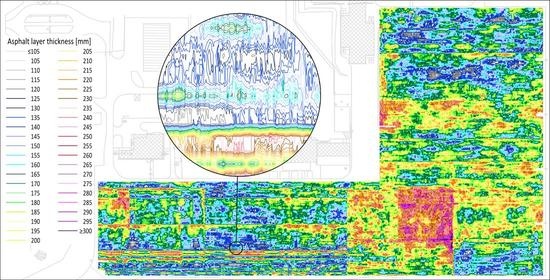
Based on the analysis of GPR data, the total asphalt layer thickness was determined at 597,348 measurement points. The total asphalt layer thickness ranged from a minimum of 55 mm to a maximum of 371 mm. The collected asphalt layer thickness data were additionally processed and x, y, and z coordinates were assigned for all measurement points according to the instructions in Chapter 2. A 3D model of the asphalt layers (MC1) was created from the measurement points by Delaunay triangulation using AutoCAD Civil 3D software. The MC1 model is graphically represented on a contour map—i.e., the points with the same asphalt layer thickness are connected by contour lines (
Figure 8). The contour lines have an equidistance value of 5 mm, which is considered accurate enough for the rehabilitation projects, although other equidistance values can be used if necessary.
In addition to the MC1 model, four other models were created—MC2, MC3, MC4, and MC5 (
Figure 9,
Figure 10,
Figure 11 and
Figure 12). All models were created based on identical data collected by the measurement described above, but they differ in the number of points considered in their creation. By omitting a specific longitudinal series of points, a simulation to determine the total asphalt layer thickness was performed with a smaller number of survey lines at a greater mutual spacing. The number of survey lines and their mutual spacing, as well as the number of points used to create a particular model, are presented in
Table 2, which shows the effect of the number of survey points on the representation of asphalt layer thickness and the accuracy of a particular model.
To determine the accuracy of the model, asphalt layer thickness values obtained by coring were compared to the values shown on the contour map. The asphalt layer thickness values on the map were determined by the nearest contour line at the core location. The relative error of the thickness values presented on the map was calculated as the ratio between the absolute error (the difference between the thickness on the map and that of the core) and the core thickness.
The MC1 model with a distance of 1 m between survey lines resulted in relative errors ranging from 0.0% to 5.6%, with a mean error of 1.5% (
Figure 13). This shows the high accuracy of the created 3D model.
The MC2 model with a distance of 2 m between survey lines resulted in relative errors ranging from 0.0% to 18.5%, with a mean error of 6.6% (
Figure 14).
The MC3 model with a distance of 3 m between survey lines resulted in relative errors ranging from 0.0% to 24.2%, with a mean error of 4.6% (
Figure 15).
The MC4 model with a distance of 4 m between survey lines resulted in relative errors ranging from 0.0% to 24.2%, with a mean error of 7.4% (
Figure 16).
The MC5 model with a distance of 5 m between survey lines resulted in relative errors ranging from 0.0% to 14.5%, with a mean error of 6.5% (
Figure 17).
The accuracy of the GPR measurement was determined by comparing the thicknesses measured on the cores with those from the GPR data. Only three cores (3, 15, and 22) were placed on survey lines, and the relative errors of the GPR measurement there ranged from 0.0% to 3.1% (
Figure 13,
Table 3).
To get a better insight into the reason why the errors in the models are larger than the GPR measurement errors, the distances between the cores and the nearest survey line were measured and then compared to the relative errors of the model. The result was that the average distance between cores closest to the survey lines was 0.23 m for the MC1 model, while the average distance between cores farthest from the survey lines was 1.10 m for the MC5 model (
Table 3). The smallest average relative errors found in the MC1 and MC3 models coincide with the smallest average distances between cores and survey lines.
As expected, the comparison of the measured distances and the relative errors of the model showed that the relative error of the model increases with increasing distance between the core and the survey line (
Table 3). However, the largest relative error, 24.2%, was not registered at the farthest core, but at core 19, which was 1.09 m away from the survey line in the MC3 and MC4 models. The most distant core 10 (model MC5) showed a relative error of 12.5%. Since the largest error of the model was not recorded at the furthest point, other influencing factors that may have affected the error occurring at core 19 were considered. It was found that within a 3.0 m radius of Core 19, there is a significant variation in asphalt layer thickness from 120 to 225 mm (
Figure 8,
Figure 9,
Figure 10,
Figure 11 and
Figure 12).
Contour maps provide a detailed representation of asphalt layer thickness and allow determination of model accuracy but are not suitable for defining homogeneous areas used in selection of rehabilitation technology. Maps with bands are more suitable for defining homogeneous areas because the bands represent the pavement area with a specific range of asphalt layer thickness. Six bands (
Table 4) were defined to determine the effect of the number of survey lines on the size of the homogeneous areas on each of the five 3D models (
Figure 18,
Figure 19,
Figure 20,
Figure 21 and
Figure 22). Band B1 includes all asphalt layer thickness values less than 100 mm. Bands B2–B5 include thickness values from 100 to 300 mm, with each band being 50 mm. Band B6 includes all asphalt layer thickness values greater than 300 mm.
The results in
Table 4 and
Table 5 show that the asphalt layer thicknesses on the apron are mostly between 150 and 200 mm, while their area percentage varies between 61.98% and 65.55% depending on the 3D model. Asphalt layer thicknesses below 100 mm and above 300 mm have the lowest percentages of total apron area (≤0.04%). The differences in surface area between the same bands in different models are not significant. The largest difference in surface area between the same bands was found in the MC1 and MC5 models. The differences in surface area between the two models in band B2 and band B3 are 3.37% and 3.57%, respectively.
4. Discussion
The classical two-dimensional representation of asphalt layer thickness is not satisfactory for the rehabilitation plans of wide surfaces, such as airfield pavements, because it is necessary to know the thickness profile over the entire surface. Therefore, a spatial representation of asphalt layer thickness is more useful on such surfaces. The spatial representation is usually achieved based on data collected by 3D GPR. However, it is also possible based on GPR data, but with additional activities. Additional activities are related to GPR data collection on more parallel survey lines that must cover the whole area under consideration, definition of the y-coordinate (a lateral displacement between the starting and adjacent survey lines) on all measurement points and creation of the 3D model. The main disadvantage of such a method is that it is time consuming; it requires a large number of survey lines, which can be a problem at airports where measurements have to be made at short intervals between regular aircraft operations without airport closure.
3D models of asphalt layer thickness can be displayed on contour maps or maps with bands. The different ways of representing asphalt layer thickness allow researchers and designers to better determine homogeneous areas, which is important for the proper selection of pavement rehabilitation technology. Specialized software allows the representation of 3D models with contours with different equidistance values and bands with different ranges of layer thickness. In this research, the division of the bands into ranges of 50 mm was chosen. This division of the bands allows the analysis of the existing pavement structure with sufficient accuracy and allows the possibility to choose the optimal rehabilitation solution. It should be emphasized that such a division of the bands is particularly important when there is no possibility to change the vertical alignment of the surface to be rehabilitated. Two cases should be distinguished. The first case concerns pavements with a total thickness of asphalt layers greater than the thickness of the newly planned layers. In this case, when the portion of existing layers are milled off, a certain minimum thickness of them must remain (50 mm). If the bands are created with a range of 50 mm, it is possible to estimate the area with a thickness of asphalt layers smaller than the specified 50 mm. On such areas it will be necessary to completely remove the asphalt layers and rehabilitate the subgrade. The second case relates to the asphalt overlay on the concrete pavement, which is usually made of the asphalt concrete AC 16 surf type with a minimum technological thickness of 42 mm. In practice, the thickness of this layer is usually 50 mm. If the thickness of the existing overlay is less than 50 mm, bands with a range of 50 mm provide information about the need to remove part of the concrete pavement.
Of course, it is possible to make divisions in bands with a smaller range, but such a choice is suitable for smaller areas where there are significant variations in the thickness of asphalt layers. Finer division, e.g., the range of 10 mm, leads to many homogeneous areas with smaller dimensions (smaller share in the total area of the apron, large scatter).
The number of survey lines affects model accuracy, but is not the only factor, as the model with the lowest number of survey lines is not the least accurate. Accuracy is affected by the distance between the core and the survey line, while local variations in layer thickness can also have a significant impact. The accuracy of the model is also affected by the triangulation procedure. Because of the regular square grid of points in the longitudinal and transverse directions, triangulation forms triangles simply by connecting points on adjacent lines. The elevation of any point on the triangulated surface is determined by interpolating the elevations of the vertices of the triangles. If the variations in the asphalt layer thickness are small, i.e., the section is homogeneous, then the influence of triangulation on the accuracy of the 3D model is smaller.
The large spacing between survey lines reduces the time required to collect and process the GPR data. If the distance between the survey lines is increased, there is a risk that significant local variations in thickness will remain undetected. Similarly, when the survey line spacing is large, if the location of the local variation in layer thickness coincides with the location of the survey line, the effect of the local variation will be visible over a larger area due to the triangulation process described previously.
The high accuracy of the 3D model suggests that such an approach to data analysis, processing and representation is satisfactory and can compensate the 3D GPR.
5. Conclusions
3D models of asphalt layers provide a clear insight into the variations of asphalt layer thickness in longitudinal and transverse directions. This research analyses the accuracy of different 3D models of asphalt layers using Airport Pula apron as an example. A total of five 3D models were created based on the different number of survey lines in which GPR data were collected and subsequently presented on contour maps or maps with bands. The different numbers of survey lines simulated the smaller or larger number of survey points that were considered in the creation of the 3D model.
Contour maps and cores were used to analyze the accuracy of the 3D models. As expected, it was found that the relative error of the 3D model was lowest at the narrowest survey line distance of 1 m and highest at the 4.0 m distance. It was found that the accuracy of a 3D model depends primarily on the accuracy of the GPR measurement, the distance of the core from the survey line—i.e., triangulation process—but also on the local thickness variations.
Maps with bands provided a representation of homogeneous surfaces with respect to the range of asphalt layer thickness. It was found that the size of certain homogeneous surfaces did not vary much considering the number of survey lines used in the creation of the 3D model.
The results of the analysis showed that the previously described methodology of GPR data collection, processing and spatial representation can be applied to airfield asphalt pavements with high accuracy. Furthermore, if the GPR measurement, data processing and interpretation have to be performed in the shortest possible time, a smaller number of survey lines can be selected, resulting in a slightly lower accuracy of the 3D model. The research has shown that GPR data can be initially collected on survey lines spaced more than 1.0 m apart, assuming that the observed section does not have significant variations in asphalt layer thickness as a result of different construction histories. The number of survey lines, and therefore the accuracy of the model, should be adjusted to suit the purpose of the research.
Author Contributions
Conceptualization, Š.B., I.S. and J.D.; methodology, Š.B. and I.S.; software, Š.B., I.S. and J.D.; validation, Š.B., I.S., J.D. and T.R.; formal analysis, Š.B., I.S. and J.D.; investigation, Š.B., I.S., J.D. and T.R.; resources, T.R.; data curation, Š.B., I.S. and J.D.; writing—original draft preparation, Š.B., and I.S.; writing—review and editing, Š.B. and I.S.; visualization, Š.B. and I.S.; supervision, J.D. and T.R.; project administration, T.R.; funding acquisition, T.R. All authors have read and agreed to the published version of the manuscript.
Funding
This research was funded by UNIVERSITY OF ZAGREB, CROATIA based on the decision on the distribution of advances for the basic financing of scientific and artistic activities, referenced as 402-08/19-03/17.
Data Availability Statement
Data available from the authors on request.
Conflicts of Interest
The authors declare no conflict of interest.
References
- Loizos, A.; Plati, C. Accuracy of pavement thicknesses estimation using different ground penetrating radar analysis approaches. NDT E Int. 2007, 40, 147–157. [Google Scholar] [CrossRef]
- Singh, A.; Sharma, A.; Chopra, T. Analysis of The Flexible Pavement Using Falling Weight Deflectometer for Indian National Highway Road Network. Transp. Res. Procedia 2020, 48, 969–3979. [Google Scholar] [CrossRef]
- Zhang, D.; Zou, Q.; Lin, H.; Xu, X.; He, L.; Gui, R.; Li, Q. Automatic pavement defect detection using 3D laser profiling technology. Autom. Constr. 2018, 96, 350–365. [Google Scholar] [CrossRef]
- Solla, M.; Lagüela, S.; González-Jorge, H.; Arias, P. Approach to identify cracking in asphalt pavement using GPR and infrared thermographic methods: Preliminary findings. NDT E Int. 2014, 62, 55–65. [Google Scholar] [CrossRef]
- Solla, M.; Lorenzo, H.; Martínez-Sánchez, J.; Pérez-Gracia, V. Applications of GPR in association with other non-destructive testing methods in surveying of transport. In Civil Engineering Applications of Ground Penetrating Radar, 1st ed.; Benedetto, A., Pajewski, L., Eds.; Springer International Publishing: Bern, Switzerland, 2015; pp. 327–342. [Google Scholar]
- Pajewski, L.; Fontul, S.; Solla, M. Ground-penetrating radar for the evaluation and monitoring of transport infrastructures. In Innovation in Near-Surface Geophysics: Instrumentation, Application, and Data Processing Methods, 1st ed.; Persico, R., Piro, S., Linford, N., Eds.; Elsevier: Amsterdam, The Netherlands, 2018; pp. 341–398. [Google Scholar]
- Hu, J.; Pavana, K.R.V.; White, D.J.; Beresnev, I. Pavement thickness and stabilised foundation layer assessment using ground-coupled GPR. Nondestruct. Test. Eval. 2015, 31, 1–21. [Google Scholar] [CrossRef]
- Agred, K.; Klysz, G.; Balayssac, J.-P. Location of reinforcement and moisture assessment in reinforced concrete with a double receiver GPR antenna. Constr. Build. Mater. 2018, 188, 1119–1127. [Google Scholar] [CrossRef]
- Zhao, S.; Al-Qadi, I. Pavement drainage pipe condition assessment by GPR image reconstruction using FDTD modeling. Constr. Build. Mater. 2017, 154, 1283–1293. [Google Scholar] [CrossRef]
- Wang, S.; Al-Qadi, I.L.; Cao, Q. Factors Impacting Monitoring Asphalt Pavement Density by Ground Penetrating Radar. NDT E Int. 2020, 115, 102296. [Google Scholar] [CrossRef]
- Liu, H.; Deng, Z.; Han, F.; Xia, Y.; Liu, Q.H.; Sato, M. Time-frequency analysis of air-coupled GPR data for identification of delamination between pavement layers. Constr. Build. Mater. 2017, 154, 1207–1215. [Google Scholar] [CrossRef]
- Zhang, J.; Zhang, C.; Lu, Y.; Zheng, T.; Dong, Z.; Tian, Y.; Jia, Y. In-situ recognition of moisture damage in bridge deck asphalt pavement with time-frequency features of GPR signal. Constr. Build. Mater. 2020, 244, 118295. [Google Scholar] [CrossRef]
- Pedret Rodes, J.; Martínez-Sánchez, J.; Pérez-Gracia, V. GPR Spectra for Monitoring Asphalt Pavements. Remote Sens. 2020, 12, 1749. [Google Scholar] [CrossRef]
- Al-Qadi, I.L.; Lahouar, S.; Jiang, K.; McGhee, K.K.; Mokarem, D. Accuracy of Ground-Penetrating Radar for Estimating Rigid and Flexible Pavement Layer Thicknesses. Transp. Res. Rec. J. Transp. Res. Board 2005, 1940, 69–78. [Google Scholar] [CrossRef]
- Al-Qadi, I.L.; Lahouar, S.; Loulizi, A. Ground-Penetrating Radar Calibration at the Virginia Smart Road and Signal Analysis to Improve Prediction of Flexible Pavement Layer Thicknesses; Technical Report No. FHWA/VTRC 05-CR7; Virginia Tech Transportation Institute: Charlottesville, Virginia, 2005. [Google Scholar]
- Flintsch, G.W.; Al-Qadi, I.L.; Loulizi, A.; Lahouar, S.; McGhee, K.; Clark, T. Field Investigation of High Performance Pavements in Virginia; Technical Report, Report No. VTRC 05-CR9; Virginia Tech Transportation Institute: Charlottesville, Virginia, 2005. [Google Scholar]
- Holzschuher, C.; Lee, H.S.; Greene, J. Accuracy and Repeatability of Ground Penetrating Radar for Surface Layer Thickness Estimation of Florida Roadways; Technical Report No. FL/DOT/SMO/07-505; Florida Department of Transportation, State Material Office: Gainesville, FL, USA, 2007.
- Ožbolt, M.; Rukavina, T.; Domitrović, J. Comparison of the Pavement Layers Thickness Measured by Georadar and Conventional Methods—Examples from Croatia. Balt. J. Road Bridge. Eng. 2012, 7, 30–35. [Google Scholar] [CrossRef]
- Domitrović, J.; Rukavina, T.; Bezina, Š.; Stančerić, I. Mapping of Runway Pavement Layers Thickness by GPR. In Proceedings of the International Conference on Sustainable Materials, Systems and Structures (SMSS2019)—Challenges in Design and Management of Structures, Rovinj, Croatia, 20–22 March 2019; Ivanković, A.M., Kušter Marić, M., Strauss, A., Kišiček, T., Eds.; RILEM Publications, S.A.R.L.: Paris, France, 2019; pp. 208–215. [Google Scholar]
- Al-Qadi, I.L.; Lahouar, S.; Loulizi, A. Ground Penetrating Radar Evaluation for Flexible Pavement Thickness Estimation. In Proceedings of the Pavement Evaluation Conference, Roanoke, VA, USA, 21–25 October 2002. [Google Scholar]
- Plati, C.; Loizos, A.; Gkyrtis, K. Integration of non-destructive testing methods to assess asphalt pavement thickness. NDT E Int. 2020, 115, 102292. [Google Scholar] [CrossRef]
- Moropoulou, A.; Avdelidis, N.P.; Koui, M.; Aggelopoulos, A.; Karmis, P. Infrared thermography and ground penetrating radar for airport pavements assessment. Nondestruct. Test. Eval. 2002, 18, 37–42. [Google Scholar] [CrossRef]
- Malvar, L.J. Detecting Voids under Pavements: Update on Approach of U.S. Department of Defense. Transp. Res. Rec. J. Transp. Res. Board 2010, 2170, 28–35. [Google Scholar] [CrossRef]
- Graczyk, M.; Krysiński, L.; Topczewski, Ł.; Sudyka, J. The Use of Three-dimensional Analysis of GPR Data in Evaluation of Operational Safety of Airfield Pavements. Transp. Res. Procedia 2016, 14, 3704–3712. [Google Scholar] [CrossRef] [Green Version]
- Saarenketo, T. NDT transportation. In Ground Penetrating Radar: Theory and Applications, 1st ed.; Jol, H.M., Ed.; Elsevier: Amsterdam, The Netherlands, 2009; pp. 395–444. [Google Scholar]
- Eide, E.; Sandnes, P.A.; Nilssen, B.; Tjora, S. Airfield Runway Inspection Using 3 Dimensional GPR. In Proceedings of 3rd International Workshop on Advanced Ground Penetrating Radar IWAGPR 2005; Delft, The Netherland, 2–3 May 2005, Lambot, S., Gorriti, A.G., Eds.; Institute of Electrical and Electronics Engineers: Delft, The Netherlands, 2005; pp. 87–91. [Google Scholar]
- Domitrović, J.; Bezina, Š.; Stančerić, I.; Rukavina, T. 3D modelling of asphalt overlays based on GPR data. Int. J. Pavement Eng. submitted for publication.
- Maser, K.R.; Scullion, T. Automated Detection of Pavement Layer Thicknesses and Subsurface Moisture Using Ground Penetrating Radar. Transp. Res. Rec. 1991, 1344, 22–30. [Google Scholar]
- Daniels, D.J. Ground Penetrating Radar, 2nd ed.; The Institution of Electrical Engineering: London, UK, 2004; p. 90. [Google Scholar]
- Saarenketo, T.; Scullion, T. Road evaluation with ground penetrating radar. J. Appl. Geophys. 2000, 43, 119–138. [Google Scholar] [CrossRef]
- Geophysical Survey Systems, Inc. Available online: https://www.geophysical.com/wp-content/uploads/2017/11/GSSI-RADAN-6_6-Manual.pdf (accessed on 18 February 2021).
Figure 1.
Pula Airport apron with pavement distresses.
Figure 1.
Pula Airport apron with pavement distresses.
Figure 2.
Measurement vehicle at the Pula Airport with Ground-penetrating radar (GPR) antennas.
Figure 2.
Measurement vehicle at the Pula Airport with Ground-penetrating radar (GPR) antennas.
Figure 3.
(a) Metal plates; (b) electromagnetic (EM) wave reflection on radargram.
Figure 3.
(a) Metal plates; (b) electromagnetic (EM) wave reflection on radargram.
Figure 4.
Scheme of electromagnetic wave transmission to the pavement.
Figure 4.
Scheme of electromagnetic wave transmission to the pavement.
Figure 5.
Interpretation of the collected GPR data by 1 GHz antenna: (a) radargram; (b) layer depth determination.
Figure 5.
Interpretation of the collected GPR data by 1 GHz antenna: (a) radargram; (b) layer depth determination.
Figure 6.
The procedure for creating 3D model of an asphalt layer: (a) 3D points; (b) 3D model with triangulated regular square grid; (c) 3D model with contours.
Figure 6.
The procedure for creating 3D model of an asphalt layer: (a) 3D points; (b) 3D model with triangulated regular square grid; (c) 3D model with contours.
Figure 7.
Location of core samples on the apron.
Figure 7.
Location of core samples on the apron.
Figure 8.
MC1 model represented with contours.
Figure 8.
MC1 model represented with contours.
Figure 9.
MC2 model represented with contours.
Figure 9.
MC2 model represented with contours.
Figure 10.
MC3 model represented with contours.
Figure 10.
MC3 model represented with contours.
Figure 11.
MC4 model represented with contours.
Figure 11.
MC4 model represented with contours.
Figure 12.
MC5 model represented with contours.
Figure 12.
MC5 model represented with contours.
Figure 13.
Model MC1—asphalt layer thickness and relative error in the core locations.
Figure 13.
Model MC1—asphalt layer thickness and relative error in the core locations.
Figure 14.
Model MC2—asphalt layer thickness and relative error in the core locations.
Figure 14.
Model MC2—asphalt layer thickness and relative error in the core locations.
Figure 15.
Model MC3—asphalt layer thickness and relative error in the core locations.
Figure 15.
Model MC3—asphalt layer thickness and relative error in the core locations.
Figure 16.
Model MC4—asphalt layer thickness and relative error in the core locations.
Figure 16.
Model MC4—asphalt layer thickness and relative error in the core locations.
Figure 17.
Model MC5—asphalt layer thickness and relative error in the core locations.
Figure 17.
Model MC5—asphalt layer thickness and relative error in the core locations.
Figure 18.
MC1 model represented with bands.
Figure 18.
MC1 model represented with bands.
Figure 19.
MC2 model represented with bands.
Figure 19.
MC2 model represented with bands.
Figure 20.
MC3 model represented with bands.
Figure 20.
MC3 model represented with bands.
Figure 21.
MC4 model represented with bands.
Figure 21.
MC4 model represented with bands.
Figure 22.
MC5 model represented with bands.
Figure 22.
MC5 model represented with bands.
Table 1.
Parameters and filters that were used during the data collection.
Table 1.
Parameters and filters that were used during the data collection.
| Parameters and Filters | Variable | 1 GHz Antenna | 2 GHz Antenna |
|---|
| Position/Range | Range [ns] | 20 | 15 |
| Position [ns] | 96 | 96 |
| Range gain | Point | 1 | 1 |
| Number of points | 1 | 1 |
| Value | 13 | 17 |
| FIR filter | Low pass [MHz] | 5000 | 6000 |
| High pass [MHz] | 300 | 300 |
| Filter type | boxcar | boxcar |
| IIR filter | Horizontal low pass [scans] | 0 | 0 |
| Horizontal high pass [scans] | 0 | 0 |
| Vertical low pass [MHz] | 0 | 0 |
| Vertical high pass [MHz] | 0 | 0 |
Table 2.
Settings of 3D models with contours.
Table 2.
Settings of 3D models with contours.
| Model Settings | 3D Models |
|---|
| MC1 | MC2 | MC3 | MC4 | MC5 |
|---|
| Distance between survey line [m] | 1 | 2 | 3 | 4 | 5 |
| Number of survey lines | 247 | 125 | 84 | 63 | 51 |
| Number of points | 597,348 | 303,562 | 203,343 | 153,788 | 125,560 |
| Contour equidistance [mm] | 5 | 5 | 5 | 5 | 5 |
Table 3.
Distance between core samples and survey line in different models and relative error.
Table 3.
Distance between core samples and survey line in different models and relative error.
| Core Sample | Distance between Core and Survey Line [m] |
|---|
| MC1 | MC2 | MC3 | MC4 | MC5 |
|---|
| 1 | 0.43 | 0.43 | 0.43 | 0.43 | 1.43 |
| 2 | 0.37 | 0.63 | 0.37 | 1.36 | 1.63 |
| 3 | 0.00 | 1.00 | 0.00 | 1.00 | 2.00 |
| 4 | 0.40 | 0.40 | 0.40 | 1.60 | 0.60 |
| 5 | 0.40 | 0.40 | 0.40 | 0.40 | 0.40 |
| 6 | 0.33 | 0.33 | 0.67 | 0.33 | 1.33 |
| 7 | 0.26 | 0.26 | 0.74 | 1.74 | 1.26 |
| 8 | 0.09 | 0.91 | 0.09 | 1.09 | 1.09 |
| 9 | 0.24 | 0.24 | 0.76 | 1.76 | 0.76 |
| 10 | 0.21 | 0.79 | 0.21 | 0.79 | 2.21 |
| 11 | 0.25 | 0.75 | 0.75 | 1.25 | 0.25 |
| 12 | 0.26 | 0.26 | 1.26 | 0.26 | 1.26 |
| 13 | 0.06 | 0.06 | 0.94 | 0.06 | 0.94 |
| 14 | 0.50 | 0.50 | 0.50 | 0.50 | 0.50 |
| 15 | 0.00 | 1.00 | 0.00 | 1.00 | 1.00 |
| 16 | 0.25 | 0.25 | 0.25 | 1.75 | 1.25 |
| 17 | 0.50 | 0.50 | 0.50 | 1.50 | 0.50 |
| 18 | 0.03 | 0.97 | 0.03 | 0.97 | 2.03 |
| 19 | 0.09 | 0.91 | 1.09 | 1.09 | 0.09 |
| 20 | 0.14 | 0.86 | 0.14 | 1.14 | 0.86 |
| 21 | 0.23 | 0.77 | 0.23 | 1.23 | 0.77 |
| 22 | 0.00 | 1.00 | 0.00 | 1.00 | 2.00 |
| Average | 0.23 | 0.60 | 0.44 | 1.01 | 1.10 |
Table 4.
Band surface areas.
Table 4.
Band surface areas.
Band
Label | Asphalt Layers Thickness
[mm] | Area [m2] |
|---|
| MC1 | MC2 | MC3 | MC4 | MC5 |
|---|
| B1 | <100 | 24.58 | 8.49 | 20.89 | 17.10 | 1.44 |
| B2 | 100–150 | 13,144.01 | 12,179.82 | 12,119.81 | 13,406.81 | 11,154.58 |
| B3 | 150–200 | 36,568.32 | 37,835.70 | 38,322.33 | 36,576.57 | 38,676.12 |
| B4 | 200–250 | 8561.50 | 8354.39 | 7863.45 | 8330.34 | 8486.47 |
| B5 | 250–300 | 691.45 | 618.36 | 655.45 | 667.93 | 672.51 |
| B6 | ≥300 | 13.62 | 6.72 | 21.55 | 4.73 | 12.36 |
Table 5.
Band surface share in the total apron area.
Table 5.
Band surface share in the total apron area.
Band
Label | Asphalt Layers Thickness
[mm] | Area [m2] |
|---|
| MC1 | MC2 | MC3 | MC4 | MC5 |
|---|
| B1 | <100 | 0.04 | 0.01 | 0.04 | 0.03 | 0.00 |
| B2 | 100–150 | 22.28 | 20.64 | 20.54 | 22.72 | 18.91 |
| B3 | 150–200 | 61.98 | 64.12 | 64.95 | 61.99 | 65.55 |
| B4 | 200–250 | 14.51 | 14.16 | 13.33 | 14.12 | 14.38 |
| B5 | 250–300 | 1.17 | 1.05 | 1.11 | 1.13 | 1.14 |
| B6 | ≥300 | 0.02 | 0.01 | 0.04 | 0.01 | 0.02 |
| Publisher’s Note: MDPI stays neutral with regard to jurisdictional claims in published maps and institutional affiliations. |
© 2021 by the authors. Licensee MDPI, Basel, Switzerland. This article is an open access article distributed under the terms and conditions of the Creative Commons Attribution (CC BY) license (http://creativecommons.org/licenses/by/4.0/).


