Article

New Orthophoto Generation Strategies from UAV and Ground Remote Sensing Platforms for High-Throughput Phenotyping

1
Lyles School of Civil Engineering, Purdue University, West Lafayette, IN 47907, USA
2
School of Electrical and Computer Engineering, Purdue University, West Lafayette, IN 47907, USA
*
Author to whom correspondence should be addressed.
Remote Sens. 2021, 13(5), 860; https://doi.org/10.3390/rs13050860
Submission received: 14 January 2021 / Revised: 22 February 2021 / Accepted: 24 February 2021 / Published: 25 February 2021
(This article belongs to the Special Issue UAV Imagery for Precision Agriculture)

Abstract

:
Remote sensing platforms have become an effective data acquisition tool for digital agriculture. Imaging sensors onboard unmanned aerial vehicles (UAVs) and tractors are providing unprecedented high-geometric-resolution data for several crop phenotyping activities (e.g., canopy cover estimation, plant localization, and flowering date identification). Among potential products, orthophotos play an important role in agricultural management. Traditional orthophoto generation strategies suffer from several artifacts (e.g., double mapping, excessive pixilation, and seamline distortions). The above problems are more pronounced when dealing with mid- to late-season imagery, which is often used for establishing flowering date (e.g., tassel and panicle detection for maize and sorghum crops, respectively). In response to these challenges, this paper introduces new strategies for generating orthophotos that are conducive to the straightforward detection of tassels and panicles. The orthophoto generation strategies are valid for both frame and push-broom imaging systems. The target function of these strategies is striking a balance between the improved visual appearance of tassels/panicles and their geolocation accuracy. The new strategies are based on generating a smooth digital surface model (DSM) that maintains the geolocation quality along the plant rows while reducing double mapping and pixilation artifacts. Moreover, seamline control strategies are applied to avoid having seamline distortions at locations where the tassels and panicles are expected. The quality of generated orthophotos is evaluated through visual inspection as well as quantitative assessment of the degree of similarity between the generated orthophotos and original images. Several experimental results from both UAV and ground platforms show that the proposed strategies do improve the visual quality of derived orthophotos while maintaining the geolocation accuracy at tassel/panicle locations.

Graphical Abstract

1. Introduction

Modern mobile mapping systems, including unmanned aerial vehicles (UAVs) and ground platforms (e.g., tractors and robots), are becoming increasingly popular for digital agriculture. These systems can carry a variety of sensors, including imaging systems operating in different spectral ranges (e.g., red–green–blue, multispectral/hyperspectral, and thermal cameras that use either frame or push-broom imaging) and LiDAR scanners. Advances in sensor and platform technologies are allowing for the acquisition of unprecedented high-geometric-resolution data throughout the growing season. Among possible applications, high-throughput phenotyping for advanced plant breeding is benefiting from the increased geometric and temporal resolution of acquired data. Remote sensing data from modern mobile mapping systems have been successfully used for field phenotyping [1] and crop monitoring [2,3], replacing many of the traditional in-field manual measurements. For example, UAV imagery and orthophotos have been used to extract various plant traits such as plant height, canopy cover, vegetation indices, and leaf area index (LAI) [4,5,6,7,8,9,10,11]. Original imagery captured by either frame cameras or push-broom scanners is impacted by perspective projection geometry (e.g., non-uniform scale and relief displacement), lens distortions, and trajectory-induced artifacts (e.g., sensor tilt artifacts in frame camera imagery and wavy pattern in acquired scenes by push-broom scanners). Therefore, derived phenotyping traits from the original imagery have to be corrected for these deformations to establish the corresponding locations in the mapping/field reference frame. High-resolution orthophotos, which are image-based products that compensate for these deformations, are increasingly used in machine vision/learning algorithms for deriving geolocated phenotypic traits [12].
Orthophoto generation from the original imagery requires the internal and external characteristics of the imaging sensors—commonly known as the interior orientation parameters (IOP) and exterior orientation parameters (EOP), respectively—as well as a digital surface model (DSM) of the mapped surface. The key advantage of derived orthophotos is correcting for various image deformations (i.e., those caused by perspective projection, lens distortions, and perturbed trajectory), thus producing map-like images where identified traits are directly available in the mapping/field reference frame. Orthophoto generation strategies can be categorized as either direct or indirect approaches [13]. For the direct approach, the spectral signature assignment for the different orthophoto cells proceeds through forward projection from the image pixels onto the DSM and then to the orthophoto. The indirect approach, on the other hand, starts with a backward projection from the DSM-based elevation of a given orthophoto cell to the corresponding location in the original image, where the spectral signature is interpolated for and assigned to the orthophoto cell in question. The key disadvantages of the direct approach include the complex, iterative procedure for forward image to DSM projection and having some orthophoto cells with unassigned spectral signatures. The latter problem, which is caused by variation in the ground sampling distance (GSD) of the imaging sensor relative to the cell size of the orthophoto, can be mitigated by an interpolation procedure following the forward projection step. The complexity of the forward projection procedure increases when dealing with an object space that exhibits several instances of sudden elevation discontinuities. Such discontinuities are quite common in agricultural fields, especially those in breeding trials, where we have different genotypic traits that lead to various elevations for neighboring plots (as shown in Figure 1a). The shortcoming of the indirect approach for orthophoto generation, which is easier to implement, is its susceptibility to the double mapping problem, i.e., not considering potential occlusions resulting from relief displacement (as depicted in Figure 1b). Problems associated with direct and indirect ortho-rectification strategies are exacerbated by the increasing geometric resolution of UAV and ground imaging systems as a result of the smaller sensor-to-object distance. In other words, traditional orthophoto rectification strategies that are quite successful for high-altitude imaging systems over a relatively smooth object space are not suitable for proximal sensing of agricultural fields, especially later in the growing season, e.g., acquired imagery for establishing flowering dates where tassel and panicle detection is paramount.
This paper introduces new orthophoto generation strategies that are designed for late-season, proximal remote sensing of agricultural fields. The following section introduces the literature related to orthophoto generation. Section 3 describes the data acquisition systems and field surveys conducted to evaluate the performance of the proposed orthophoto generation strategies in Section 4. Experimental results and discussion are presented in Section 5, which is followed by a coverage of the research key findings and directions for future work.

2. Related Work

Aside from inaccurate system calibration and georeferencing parameters, factors that would impact the quality of derived orthophotos include (a) imprecise DSM, (b) pixilation and double mapping artifacts, and (c) seamline distortions. Several research efforts have been conducted, and proved successful, to improve the georeferencing and system calibration parameters of imaging systems onboard remote sensing platforms [14,15,16,17]. Imprecise DSM problems would be more pronounced when dealing with large-scale imagery over a complex object space, which is the key characteristic of late-season imaging using UAV and ground platforms over breeding trials with varying genotypes in neighboring plots (Figure 1a). Wang et al. [18] showed that the sawtooth effect (serrated edges with sharp notches) occurs in orthophotos covering urban areas when the DSM does not precisely model the building edges. They resolved this problem by matching and reconstructing linear features at the building boundaries and adding the corresponding 3D line segments to the DSM. In agricultural fields, the DSM quality is limited by its resolution and difficulty in representing individual plants and/or plant organs. Using either LiDAR or imaging sensors, it is impossible to avoid potential artifacts in the generated DSM due to environmental and sensor-related factors such as wind, repetitive pattern, ranging accuracy, and georeferencing quality.
The double mapping problem (also known as the ghost image effect) is an artifact produced by indirect ortho-rectification strategies [13]. Such an artifact occurs when the object space exhibits abrupt elevation variations. Figure 2 shows a schematic diagram of the double mapping problem. In Figure 2, both DSM/orthophoto cells s and 3 are back-projected to the same image pixel a. While the orthophoto cell 3 is assigned the correct spectral signature, this value is incorrectly duplicated at cell 1 because of the relief displacement and not considering the introduced occlusion during the indirect ortho-rectification. The same problem is encountered for DSM cells 2 and 4, which are projected to the same pixel b. This results in repeated patterns—i.e., double mapping of the same area—in the orthophoto (Figure 1b). The majority of existing techniques for handling the double mapping problem utilize the Z-buffer algorithm [19,20,21]. The Z-buffer keeps track of projected DSM cells to a given image location. When several DSM cells are projected to the same image pixel, the closest DSM cell to the perspective center of the image in question is deemed visible while the others are considered occluded. This technique is very sensitive to the GSD of the imaging sensor as it relates to the orthophoto cell size. In addition, the Z-buffer requires the introduction of pseudo points along elevation discontinuities to avoid false visibilities [13]. Kuzmin et al. [20] developed a hidden area detection algorithm for urban areas. Their approach starts with establishing polygons, which represent planar features, from the DSM point cloud. Then, the polygons are projected onto the image and visible polygons are identified based on their distance to the perspective center. Habib et al. [13] proposed an angle-based true orthophoto generation approach that sequentially checks the off-nadir angle to the line of sight connecting the perspective center and DSM cell in question. Occlusions are detected whenever there is an apparent decrease in the off-nadir angle as moving away from the nadir point. The above approaches for visibility analysis rely on having a precise DSM that is not available for large-scale imagery over agricultural fields. Therefore, eliminating double mapping in orthophotos covering agricultural fields remains a challenge.
The third challenge during orthophoto generation is the inevitable radiometric and geometric discontinuities across the seamline when transitioning from one image to another throughout the mosaicking process. Seamline optimization has been investigated to minimize such discontinuities. While radiometric differences can be minimized by digital number equalization [22,23], geometric discontinuities are harder to tackle and are the focus of several studies. Radiometric seamline optimization algorithms typically comprise two parts: (a) defining a cost function using pixel-by-pixel differences of one or more metrics, and (b) searching for the path with the lowest cost. Milgram [24] first proposed the use of grey value differences as a metric. However, this metric only reflects the difference between two rectified images at a single orthophoto cell, without considering neighborhood information. Subsequent studies proposed image gradient [25,26], normalized cross correlation [27], edge [28], image saliency [28], and distance between an orthophoto cell and object space nadir points of the images [28] as metrics for evaluating the difference between two rectified images. In terms of searching algorithms, the “Dijkstra shortest path” algorithm has been widely adopted [26,27,28]. Other algorithms, such as the “bottleneck shortest path” algorithm [29,30] and “twin-snake” model [25], also showed good performance. In addition to digital number/radiometric equalization, another equally important aspect is related to geometric manipulation to avoid having seamlines crossing salient objects in the orthophoto. Several studies have explored the use of external information for controlling seamline locations in urban areas. Chen et al. [31] used the elevation information from a DSM and applied the “Dijkstra” algorithm to guide the seamline toward lower elevation regions. Wan et al. [32] proposed the use of road network data to have the seamlines follow the centerlines of wide streets where no significant discontinuities exist. Pang et al. [33] used disparity images generated by the semi-global matching process to guide the seamlines away from building locations. For agricultural fields, high-resolution images capturing detailed plant structure are now available. However, there has been no discussion regarding seamline optimization during orthophoto generation for such applications.
With current advances in remote sensing technology and platforms, sub-centimeter resolution images over agricultural fields are becoming increasingly available. However, data processing and analysis activities are still lacking, thus not allowing the full potential of acquired remote sensing data to be exploited. The quality of UAV-based orthophotos has enabled automated identification of individual plants (i.e., facilitating plant localization and plant count derivation) using early season imagery. However, generated orthophotos are not sufficient for late-season applications such as tassel/panicle detection. Such applications require sub-centimeter-resolution and high-visual-quality images/orthophotos, where individual tassels and panicles can be identified. Guo et al. [34] detected sorghum heads from original images and used generated orthophotos only for geolocating the plots. Duan et al. [35] compared ground cover estimation using undistorted images (i.e., corrected for lens and camera distortions) and corresponding orthophotos. They concluded that ground cover estimation using orthophotos is less accurate due to the presence of the previously discussed artifacts (wind-driven ghosting effects and image mosaicking discontinuities). As an example, Figure 3 shows a portion of a UAV image over an agricultural field and corresponding orthophoto. While the RGB image has good visual quality, the orthophoto is pixelated with several discontinuities, making it difficult to identify individual leaves and tassels. In summary, the main factors affecting the quality of generated orthophotos can be summarized as follows:
  • The DSM is not precise enough to describe the covered object space (i.e., model each stalk, tassel/panicle, and leaf);
  • The visibility/occlusion of DSM cells results in double-mapped areas in the orthophoto;
  • The mosaicking process inevitably results in discontinuities across the boundary between two rectified images (i.e., at seamline locations).
These problems have been identified and discussed for decades, and significant progress has been made in generating orthophotos over urban areas. However, these techniques do not work for high-resolution images over agricultural fields. Therefore, identifying and developing strategies that improve the visual quality of orthophotos covering crop fields is crucial. This paper presents strategies for generating high-quality, large-scale orthophotos, which facilitate automated tassel/panicle detection. The main objective is striking a balance between the visual quality of tassels/panicles in generated orthophotos and their geolocation accuracy. The proposed strategy addresses the generation of a smooth DSM to achieve such balance and seamline control to avoid crossing row segments and/or individual plants. The former reduces pixilation artifacts and double-mapped areas in the derived orthophotos. The latter utilizes external information including row segment boundaries and plant locations to guide the seamlines away from tassels/panicles. In addition, a quantitative assessment approach using the scale-invariant feature transform (SIFT) matching [36] is proposed to evaluate the quality of derived orthophotos. The performance of the proposed strategies is evaluated using datasets collected by UAV and ground platforms equipped with frame cameras and push-broom scanners over maize and sorghum fields.

3. Data Acquisition Systems and Dataset Description

Several field surveys were conducted to evaluate the performance of the proposed orthophoto generation strategies on images acquired: (a) using different mobile mapping systems, including UAV and ground platforms; (b) using different sensors, including an RGB frame camera and a hyperspectral push-broom scanner with different sensor-to-object distances ranging from 40, 20, to 4 m; and (c) over breeding trials for various crops, including maize and sorghum. The following subsections cover the specifications of the data acquisition systems and platforms as well as the study site and used datasets.

3.1. Impact of Canopy on GNSS/INS-Derived Trajectory

The mobile mapping systems used in this study include UAV and ground remote sensing platforms. The UAV system, shown in Figure 4, consists of a Velodyne VLP-16 Puck Lite laser scanner, a Sony α7R III RGB frame camera, a Headwall Nano-Hyperspec VNIR push-broom hyperspectral scanner, and a Trimble APX-15 UAV v3 position and orientation unit integrating Global Navigation Satellite Systems/Inertial Navigation Systems (GNSS/INS). The RGB camera and hyperspectral scanner maintain an approximate nadir view during the data acquisition. The GNSS/INS unit provides georeferencing information (i.e., the position and attitude information of the vehicle frame at a data rate of 200 Hz). The expected post-processing positional accuracy is ±2 to ±5 cm, and the attitude accuracy is ±0.025° and ±0.08° for the roll/pitch and heading, respectively [37]. The VLP-16 scanner has 16 radially oriented laser rangefinders that are aligned vertically from +15° to −15°, leading to a total vertical field of view (FOV) of 30°. The internal mechanism rotates to achieve a 360° horizontal FOV. The scanner captures around 300,000 points per second, with a range accuracy of ±3 cm and a maximum range of 100 m [38]. The Sony α7R III has an image resolution of 42 MP with a 4.5-µm pixel size [39]. The camera is triggered by an Arduino Micro microcontroller board to capture images at 1.5-s intervals. The Headwall Nano-Hyperspec VNIR has 270 spectral bands with a wavelength range of 400 to 1000 nm and a pixel pitch of 7.4 µm [40].
The ground mobile mapping system (shown in Figure 5) is equipped with a Velodyne VLP-16 Hi-Res laser scanner, a Velodyne HDL-32E laser scanner, two FLIR Grasshopper3 RGB cameras, a Headwall Machine Vision hyperspectral push-broom scanner, and an Applanix POSLV 125 integrated GNSS/INS unit. The system is hereafter denoted as the “PhenoRover”. The RGB cameras are mounted with a forward pitch of around 15°. The hyperspectral scanner faces downwards and thus maintains a close-to-nadir view during data acquisition. For the POSLV 125, the post-processing positional accuracy is ±2 to ±5 cm, and the attitude accuracy is ±0.025° and ±0.08° for the roll/pitch and heading, respectively [41]. The VLP-16 Hi-Res has the same specifications as the UAV VLP-16 scanner with the exception that the laser beams are aligned vertically from +10° to −10°, leading to a total vertical FOV of 20°. The HDL-32E laser scanner has 32 radially oriented laser rangefinders that are aligned vertically from +10° to −30°, leading to a total vertical FOV of 40°. Similar to the other VLP scanners, the scanning mechanism rotates to achieve a 360° horizontal FOV. The range accuracy of the VLP-16 Hi-Res and HDL-32E laser scanners is ±3 and ±2 cm, respectively [42,43]. The FLIR Grasshopper3 cameras have an image resolution of 9.1 MP with a pixel size of 3.7 µm and both cameras are synchronized to capture images at a rate of 1 frame per second. The Headwall Machine Vision has 270 spectral bands with a wavelength range of 400 to 1000 nm and a pixel pitch of 7.4 µm [40]. It should be noted that the LiDAR unit onboard the UAV platform is used to derive the DSM for the ortho-rectification process.
For precise orthophoto generation, the internal and external camera characteristics (IOP and EOP) have to be established through a system calibration procedure and derived position and orientation information from the onboard GNSS/INS direct georeferencing unit. The system calibration includes the IOP estimation and evaluation of the mounting parameters (i.e., relative position and orientation) between cameras and the GNSS/INS unit. In this study, the cameras’ IOPs are estimated and refined through calibration procedures proposed in previous studies [17,44]. The USGS Simultaneous Multi-Frame Analytical Calibration (SMAC) distortion model—which encompasses the principal distance c, principal point coordinates ( x p , y p ), and radial and decentering lens distortion coefficients ( K 1 , K 2 , P 1 , P 2 )—is adopted. For the DSM generation, the mounting parameters for the LiDAR unit have to be also established. The mounting parameters for the imaging and ranging units are determined through a rigorous system calibration [15,45]. Once the mounting parameters for each system are estimated accurately, the LiDAR point cloud and images from each of the systems are georeferenced relative to a common reference frame.

3.2. Study Sites and Dataset Description

Several field surveys were carried out over two agricultural fields within Purdue University’s Agronomy Center for Research and Education (ACRE) in Indiana, USA. The two fields, shown in Figure 6, were used for maize and sorghum seed breeding trials. The planting density of the maize field was slightly higher than that of the sorghum field. For each field, UAV and PhenoRover datasets were collected on the same date. Both UAV and PhenoRover systems are capable of collecting LiDAR data as well as RGB and hyperspectral images in the same mission. For the UAV, the data acquisition missions are conducted at two flying heights: 20 and 40 m. For the PhenoRover, the sensor-to-object distance is roughly 3 to 4 m. The GSDs of the acquired images are estimated using the sensor specifications and flying height/sensor-to-object distance. For the frame camera onboard the UAV, the GSD is roughly 0.25 and 0.5 cm for the missions at 20- and 40-m flying heights, respectively. For the push-broom scanner onboard the UAV, the GSD is 2 and 4 cm for flying heights of 20 and 40 m, respectively. For the PhenoRover, the GSDs for the RGB and hyperspectral cameras are 0.2 and 0.5 cm, respectively.
In this study, UAV LiDAR point clouds from the 20-m flying height were used for DSM generation; RGB and hyperspectral images from UAV and PhenoRover were considered for orthophoto generation. Table 1 lists the datasets used in this study and reports the flight/drive-run configuration. The drive-run configuration for the PhenoRover was designed to only focus on particular rows in the field, and therefore there was no side-lap between hyperspectral scenes from neighboring drive runs. The UAV hyperspectral scenes have a relatively large GSD, which does not allow for individual tassel/panicle identification. Datasets UAV-A1, UAV-A2, and PR-A were collected over the maize field on 17 July 2020, 66 days after sowing (DAS). Based on manual flowering data collected, the maize was in the silking (R1) stage. Datasets UAV-B1, UAV-B2, and PR-B were collected over the sorghum field on 20 July 2020, 68 DAS. The sorghum was in boot stage; panicles were pushed up through the flag leaf collar by the upper stalk. Orthophotos at those times (i.e., 66/68 DAS) can serve as an input for automated tassel/panicle detection and counting, which is crucial for estimating flowering date.

4. Proposed Methodology

The proposed approach aims at generating orthophotos, which are suited for tassel and panicle detection, from acquired imagery by frame cameras and push-broom scanners. More specifically, the objectives of the proposed methodology are: (a) preserving the visual integrity of individual tassels/panicles in the generated orthophotos, (b) minimizing the tassel/panicle geolocation errors, and (c) controlling the seamlines away from the tassel/panel locations. Accordingly, the proposed methodology proceeds by smoothing the DSM to satisfy the first two objectives. Then, row segment and/or plant locations are used to control the seamline locations away from the tassels/panicles. DSM smoothing is essential for high-quality orthophoto generation from imagery acquired by frame cameras and push-broom scanners. However, due to the nature of overlap/side-lap among frame camera imagery, seamline control is critical for such imagery (i.e., since acquired imagery by push-broom scanners does not have overlap, seamline control is only necessary when mosaicking orthophotos from neighboring flight lines). For quantitative evaluation of the performance of the proposed approach, a SIFT-based matching procedure is implemented to compare the visual quality of generated orthophotos from traditional and proposed strategies to the original imagery. This section starts with a brief introduction of the mathematical model relating image and ground coordinates as well as orthophoto generation for frame cameras and push-broom scanners. Next, the proposed DSM smoothing and seamline control strategies are presented in Section 4.2 and Section 4.3, respectively. Finally, Section 4.4 describes the image quality assessment based on SIFT matching.

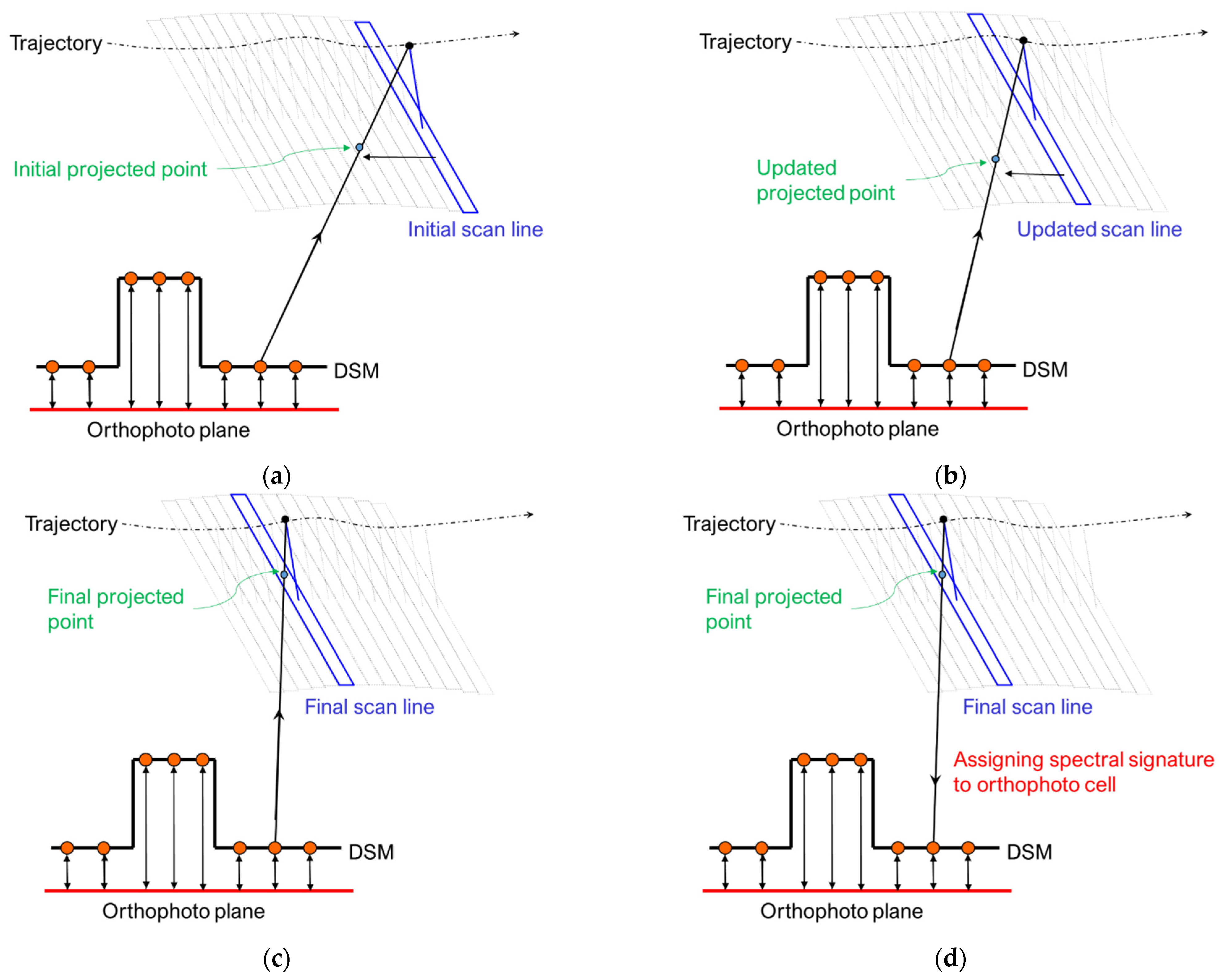
4.1. Point Positioning Equations and Ortho-Rectification for Frame Cameras and Push-Broom Scanners

The ortho-rectification generation strategy adopted in this study is the indirect approach [13], as illustrated in Figure 7. More specifically, a raster grid for the orthophoto is established along the desired datum. For each orthophoto cell, the corresponding elevation is derived from the available DSM. The 3D coordinates are then projected onto the image covering this area using the collinearity equations. The spectral signature at the image location is interpolated and assigned to the corresponding orthophoto cell. The following discussion introduces the collinearity equations for frame cameras and push-broom scanners and their usage for identifying the image location corresponding to a given object point. The discussion also deals with the selection of the appropriate image or scan line for extracting the spectral signature from frame camera imagery and push-broom scanner scenes, respectively.
For the representation of the collinearity equations, a vector connecting point “b” to point “a” relative to a coordinate system associated with point “b” is denoted as r a b . A rotation matrix transforming a vector from coordinate system “a” to coordinate system “b” is represented as   R a b . For frame cameras, we have a 2D array of light-sensitive elements in the image plane (Figure 8a). Therefore, the x and y components of the image point coordinates relative to the camera coordinate system— r i c ( t ) —have variable values depending on the angular field of view (AFOV) of the camera. For push-broom scanners, on the other hand, the image plane comprises a 1D array of light-sensitive elements. The scan line is usually orthogonal to the flight line (Figure 8b). Thus, the x component of the image point coordinates— r i c ( t ) —is constant (set to zero when the scan line is placed vertically below the perspective center). A push-broom scanner scene is established by concatenating successive acquisitions of the scan line. The scan line location in the final scene is an indication of the exposure time for that scan line. Despite this difference in the image coordinates when dealing with frame camera and push-broom scanner imagery, the collinearity equations for GNSS/INS-assisted systems take the same form as represented by Equation (1) [46]. Here, r I m is the ground coordinates of the object point I ; r i c ( t ) is the vector connecting perspective center to image point i captured by camera/scanner c at time t; λ ( i , c , t ) is the scale factor for point i captured by camera/scanner c at time t. The GNSS/INS integration establishes the position, r b ( t ) m , and rotation matrix, R b ( t ) m , of the inertial measurement unit (IMU) body frame relative to the mapping reference frame at time t . The system calibration determines the lever arm, r c b , and boresight matrix, R c b , relating the camera/scanner frame to the IMU body frame. The terms in the collinearity equations are reordered to express the image coordinates— r i c ( t ) —as functions of other parameters while removing the scale factor— λ ( i , c , t ) —by reducing the three equations to two. Given the 3D coordinates of an object point, the reformulated collinearity equations can be used to derive the corresponding image location. For frame cameras, the ground-to-image coordinate transformation is a straightforward process as we have two equations in two unknowns. The only challenge is identifying the image that captures the object point in question. Due to the large overlap and side-lap ratios associated with frame camera data acquisition, a given object point is visible in multiple images. A simple strategy is selecting the closest image based on the 2D distance from the camera location to the object point in question (i.e., the image whose object space nadir point is closest to the orthophoto cell in question).
r I m = r b ( t ) m + R b ( t ) m r c b + λ ( i , c , t ) R b ( t ) m R c b r i c ( t )
For push-broom scanners, on the other hand, the ground-to-image coordinate transformation is more complex as we are solving for both the image coordinates as well as the time of exposure (i.e., the epoch— t —at which the object point is imaged by the scanner). The conceptual basis for identifying the scan line capturing a given object point starts with an approximate exposure time— t o —and iteratively refines this time until the x -image coordinate of the projected point is equal to zero (assuming that the scan line is placed vertically below the perspective center). Figure 9 graphically illustrates this iterative procedure. First, for a given object point, its closest scan line (in 2D) is determined and denoted as the initial scan line where this point is believed to be visible. Next, the internal and external characteristics of the imaging sensor are used to back-project the point onto the initial scan line. The initial x -image coordinate of the back-projected point coordinate is used to determine an updated scan line for the next iteration. The process is repeated until the -image coordinate is as close as possible to zero. Once the correct scan line is determined, the spectral signature of the orthophoto cell is derived by resampling the neighboring spectral values along the scan line.

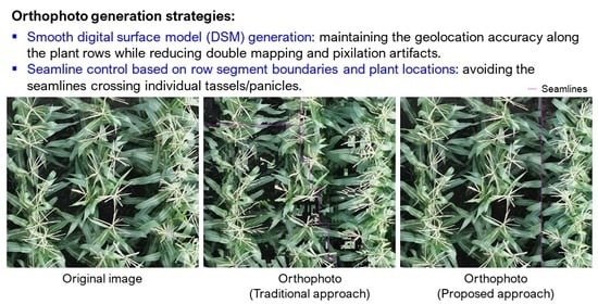
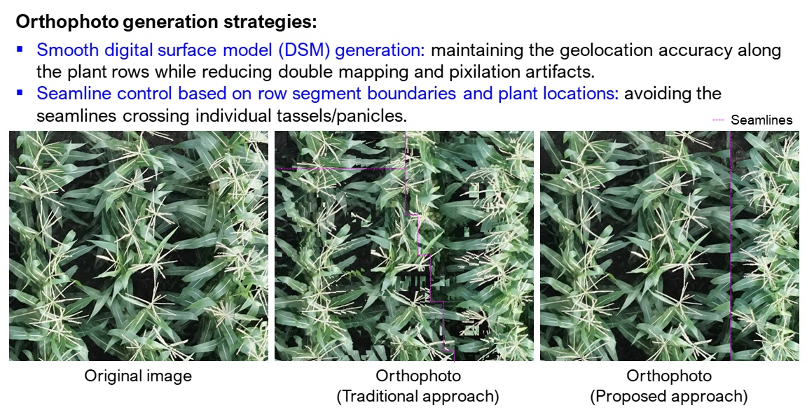
4.2. Smooth DSM Generation

This section introduces the adopted strategies for generating a smooth DSM, which strikes a balance between avoiding pixilation/double mapping artifacts and geolocation accuracy at the tassel/panicle locations. In this study, LiDAR point clouds are used as the source for DSM generation. First, a regular DSM is generated using the approach described in Lin et al. [47], where the 90th percentile of the sorted elevations within a given cell is used to represent the surface. Using the 90th percentile of the sorted elevations rather than the highest one is preferred since it reduces the noise impact. A nearest neighbor interpolation and a median filter are then applied to fill empty DSM cells and further reduce the noise impact. In agricultural fields, the derived DSM would exhibit frequent elevation variation throughout the field. Figure 10a provides a sample 90th percentile DSM where a side view of the selected area shown in the black box is presented in Figure 10d. As evident in the figure, large elevation differences may exist between neighboring DSM cells. Such variation is the main reason for pixilation and double mapping artifacts. Therefore, the DSM needs further smoothing.
The proposed smooth DSM generation approach is inspired by the cloth simulation introduced by Zhang et al. [48] for digital terrain model (DTM) generation. The conceptual basis of this approach is simulating a cloth (consisting of particles and interconnections with pre-specified rigidness) and placing it above an inverted point cloud. Then, the cloth is allowed to drop under the influence of gravity. Assuming that the cloth is soft enough to stick to the surface, the final shape of the cloth will be the DTM. In our implementation, rather than dropping the cloth on top of the inverted point cloud, the cloth is directly dropped onto the original point cloud—refer to Figure 11 for an illustration of the original cloth simulation for DTM generation and the proposed approach for smooth DSM generation. The smoothness level of the generated DSM is controlled by the preset rigidness of the interconnections among neighboring particles along the cloth. Another aspect of the cloth-based smooth DSM generation is maintaining the highest elevations, which takes place at the tassel/panicle locations, thus ensuring their geolocation accuracy. A sample of cloth-based smooth DSM and a side view of the selected area is presented in Figure 10b,d, respectively. This smoothing strategy will reduce pixilation artifacts since it eliminates sudden elevation changes throughout the field. However, double mapping problems could still exist. This problem will be more pronounced when dealing with large-scale imagery, which is the case for proximal remote sensing using UAV and ground platforms. Therefore, additional smoothing operation is necessary. In this research, we use the average elevation of the cloth-based DSM within a row segment as an additional smoothing step. To do so, the boundaries (four vertices) of the row segments are automatically extracted from LiDAR data using the strategy proposed by Lin and Habib [49]. The average elevation of the cloth-based DSM cells within each row segment is considered as the row segment elevation (i.e., the row segment elevation is assigned to all the cells enclosed by that segment). A sample of the resulting smooth DSM is shown in Figure 10c. It is hypothesized that this smoothing strategy will retain the visual quality of the original images for each row segment in the derived orthophoto. Moreover, the geolocation error is minimal at the center of the row segment where the tassels/panicles are expected. The geolocation error increases toward the row segment boundary, as illustrated in Figure 12.

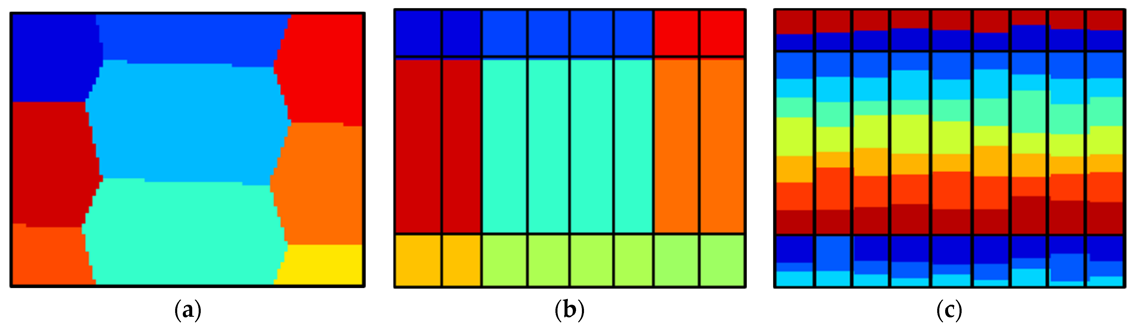
4.3. Controlling Seamline Locations Away from Tassels/Panicles

Seamlines will take place whenever neighboring spectral signatures in the orthophoto are generated using different frame camera images or push-broom scanner scenes. For frame camera images, we have significant overlap between successive images along the flight line as well as side-lap between neighboring flight lines. For push-broom scanner imagery, on the other hand, we do not have overlap between successive images along the flight lines (a push-broom scanner scene is generated by concatenating successive images along the flight line). For such scenes, a seamline will take place when transitioning between two neighboring flight lines. Therefore, the following discussion will focus on the proposed seamline control strategy for ortho-rectification of frame camera imagery. Then, the proposed strategy will be generalized to push-broom scanner scenes.
Before discussing the proposed seamline control strategy for frame cameras, we need to investigate the expected seamline locations using traditional ortho-rectification. As mentioned earlier, the used image to derive the spectral signature for a given orthophoto cell is the one that is closest in 2D to that cell. The main reason for such a strategy is ensuring the use of the image that exhibits minimal relief displacement among all images covering a particular orthophoto cell. Therefore, the seamlines in the generated orthophoto mosaic will be the Voronoi diagram established using the 2D object space locations of the perspective centers (i.e., the nadir point locations) within the image block—refer to the graphical illustration in Figure 13a. The proposed strategy imposes additional constraints on seamlines to ensure that they do not cross locations where tassels/panicles are expected. The seamline control strategy is slightly different when dealing with imagery captured by UAV and ground platforms.
For UAV imagery, the spectral signatures within a given row segment are derived from a single image. In other words, rather than using the image whose object space nadir point is closest to the orthophoto cell, we use the image that is closest to the center of a row segment to assign the spectral signatures for that row segment. Therefore, we ensure that the seamlines will not be crossing a row segment (refer to Figure 13b for a graphical illustration of the impact of using such a constraint). Adding such a constraint would lead to having some orthophoto cells using an image whose nadir point is not the closest to that cell. In other words, we might have some locations where the relief displacement minimization might not be optimal. However, given the large extent of covered area by a single UAV image and relatively short row segments, the impact of non-optimal minimization of the relief displacement will not be an issue.
For ground platforms, the image-to-object distance is significantly smaller, leading to much larger-scale, and subsequently excessive, relief displacement in the acquired imagery. In this case, ensuring that an entire row segment in the orthophoto mosaic is generated from a single image might lead to significant relief displacement artifacts. Therefore, we reduce the location constraint from the entire row segment to individual plants. In other words, the seamlines are controlled to only pass through mid-row-to-row and mid-plant-to-plant separation (refer to Figure 13c for a graphical illustration of the impact of using such a constraint). In this study, plant locations are derived from early-season UAV orthophotos through the approach proposed by Karami et al. [50]. The proposed seamline control strategy is based on defining a uv local coordinate system where the v axis is aligned along the row direction. The plant centers within this row segment are isolated. The distances along the v axis between successive plant centers are calculated. If a distance is larger than a predefined threshold, a seamline half-way between their locations is permitted. The threshold can be defined according to the size of the objects in question (i.e., tassels/panicles). However, when two neighboring plants are very close to each other, a seamline is not permitted (i.e., for close plants, a seamline is not permitted since the tassels/panicles for those plants might overlap). The orthophoto cells within each partition are assigned the spectral signature from the image whose nadir point is the closest to the center of that partition. A sample of controlled seamline locations based on this strategy is illustrated in Figure 13c.
As mentioned earlier, for push-broom scanner scenes, we do not need to worry about seamline control along the scene since successive images/rows in the scene do not have overlap. Therefore, we only need to control the seamline location between neighboring scenes. For push-broom scanners onboard ground platforms, the drive-run direction is parallel to the crop rows to have non-destructive data acquisition (i.e., the wheels of the platform have to tread through the row-to-row separation). Therefore, the seamlines between neighboring scenes can be controlled by ensuring that they do not cross the row segment. Therefore, the chosen scene for a given row segment is the one whose trajectory is closest the center of that row segment.

4.4. Orthophoto Quality Assessment

In this study, different DSM smoothing and seamline control strategies are proposed to improve the visual quality of generated orthophotos. As mentioned earlier, the visual quality is achieved by striking a balance between reducing pixilation/double mapping artifacts and ensuring geolocation accuracy at tassel/panicle locations. The visual quality is evaluated by checking the closeness of the orthophoto content to that in the original imagery. To quantitatively evaluate the visual quality of the derived orthophoto, a metric based on SIFT matching is proposed (SIFT is a feature detection and descriptor algorithm using local regions around identified interest points [36]). The hypothesis of the proposed metric is evaluating the number of matches between the original image and generated orthophoto. A larger number of matches is an indication of having an orthophoto that maintains the visual quality of the original imagery. It should be noted that this metric is intended mainly for generated orthophotos from frame imagery. For acquired imagery by a push-broom scanner, the original imagery has trajectory-induced artifacts, which should disappear in the generated orthophoto.
The image quality assessment is performed on a row segment by row segment basis for UAV frame camera images. First, a row segment is extracted from the orthophoto and the corresponding image used for assigning the spectral signatures for the row segment in question is identified. The row segment vertices in the image are derived by back-projection of the 3D coordinates of that segment using the available internal and external characteristics of the imaging sensor. The area bounded by the four vertices is then extracted from the original image. Next, the SIFT algorithm is applied to detect and match features between the segments extracted from the original image and orthophoto, as shown in Figure 14. The relative comparison of the number of matches is used to evaluate the comparative performance of the different orthophoto generation strategies. One should note that this metric should be applied on a row segment basis. For different row segments, the number of matches can be different due to the distinct patterns in the original image. For ground frame imagery, the quality control process can be carried out on a plant-by-plant basis.

5. Experimental Results and Discussion

This paper introduced different strategies for improving the quality of generated orthophotos from late-season imagery, which has been captured by frame cameras and push-broom scanners, for tassel/panicle detection. The key contributions, whose performance will be evaluated through the experimental results from real datasets covering maize and sorghum fields, are as follows:
(a)
Different approaches for smooth DSM generation, which can be used for both frame camera and push-broom scanner imagery, including the use of 90th percentile elevation within the different cells, cloth-simulation of such DSM, and elevation averaging within the row segments of cloth-based DSM;
(b)
A control strategy to avoid the seamlines crossing individual row segments within derived orthophotos from frame camera images and push-broom scanner scenes captured by a UAV platform;
(c)
A control strategy to avoid the seamlines crossing individual plant locations within derived orthophotos from frame camera images captured by a ground platform; and
(d)
Quality control metric to evaluate the visual characteristics of derived orthophotos from frame camera images captured by a UAV platform.
Section 5.1 investigates the impact of different DSM smoothing and seamline control strategies on derived orthophotos from UAV frame camera imagery over a maize field from a 20-m flying height. The quality control metric is then used to identify the optimal DSM smoothing strategy and verify the validity of the proposed seamline control approach. Next, Section 5.2 tests the performance of the best DSM smoothing strategy for orthophoto generation using UAV frame camera and push-broom scanner imagery, as well as ground push-broom scanner imagery covering maize and sorghum fields. For the UAV frame camera and push-broom scanner imagery, the respective seamline control strategy has been used. Finally, Section 5.3 evaluates the performance of the proposed seamline control strategy for orthophoto generation from ground frame camera imagery.

5.1. Impact of DSM Smoothing and Seamline Control Strategies on Derived Orthophotos from UAV Frame Camera Imagery

In this test, generated orthophotos using different DSM smoothing and seamline control strategies are inspected to decide the best DSM smoothing approach and validity of the proposed seamline control for UAV imagery. The UAV-A1 dataset—UAV frame camera imagery captured at 20-m flying height over the maize field—was used in this analysis. The captured UAV LiDAR from this flight was used for the DSM generation. One should note that an image-based DSM can be also used for orthophoto generation. However, prior research has shown that image-based 3D reconstruction techniques are more sensitive to environmental factors and face several challenges (e.g., repetitive patterns) in agricultural fields [47,51]. Therefore, LiDAR data were used for DSM generation in this study since they are more reliable. A total of three DSMs—90th percentile, cloth simulation, and average elevation within a given row segment—were generated, as shown in Figure 10. The resulting DSMs from these smoothing strategies are denoted hereafter as “90th percentile DSM”, “Cloth simulation DSM”, and “Average elevation within a row segment DSM”. In this study, the average density of the point clouds is more than 6000 points/m2, which is equivalent to an inter-point spacing of approximately 1 cm. The DSM resolution was set to 4 cm to retain the inherent level of spatial information. Two seamline control strategies were tested in this experiment. The first one is based on the 2D Voronoi network of the object space nadir points of the images covering the field—denoted hereafter as the “Voronoi network seamline control”. The second approach is based on augmenting the Voronoi network seamline control with available row segment boundary—denoted hereafter as “row segment boundary seamline control”. A total of six orthophotos were generated using different DSM smoothing and seamline control generation strategies, as listed in Table 2. The orthophotos were generated with a 0.25-cm resolution, which is approximately equal to the GSD of the UAV frame camera imagery at 20-m flying height. Figure 15 depicts portions of these orthophotos with the superimposed seamlines in yellow. As can be observed in Figure 15, insufficient DSM smoothing and Voronoi network seamline control result in orthophotos with lower visual quality. More specifically, the impact of insufficient smoothing, when using the 90th percentile DSM, is quite obvious in orthophotos i and iv, as can be seen in Figure 15a,d (pixelated, double mapping, and discontinuity artifacts—highlighted by the red circles in the zoomed-in areas). The visual quality is significantly improved using the Cloth simulation DSM, as can be seen in Figure 15b,e. However, some double-mapped areas still exist due to height variations (highlighted by the red circles in the zoomed-in areas). Using the Average elevation within a row segment DSM eliminates the double mapping issue, as shown in Figure 15c,f. As expected, Figure 15 shows that discontinuities only happen across the seamlines. While the Voronoi network seamline control allows the seamlines to cross plants locations, the row segment boundary seamline control avoids such problems. For the latter, discontinuities will not impact the identification of the individual tassels. Overall, through visual inspection, the average elevation within a row segment DSM and row segment boundary seamline control produce the best orthophoto for tassel detection (orthophoto vi in Figure 15f).
To qualitatively evaluate the geolocation accuracy of the derived orthophotos, Figure 16 illustrates the row centerlines—detected from the LiDAR data using the approach proposed by Lin and Habib [49]—on top of the six orthophotos. The row centerlines are well-aligned with the tassels in all the orthophotos, indicating the high geolocation accuracy at tassel locations. To quantitatively evaluate the performance of the proposed DSM smoothing and seamline control strategies, the introduced SIFT-based quality metric was conducted. Table 3 reports the number of established matches between the generated orthophotos from the different strategies and original images for 10 selected row segments where tassels are visible. The largest number of established matches for each row segment is in bold. As a graphical illustration example, the SIFT detection and matching results for row segment 1 are visualized in Figure 17. Closer inspection of the reported matches in Table 3 reveals that for a given seamline control strategy, the number of matches is highest when using the average elevation within a row segment DSM, lower when using the Cloth simulation DSM, and lowest when using the 90th percentile DSM. For a given DSM smoothing strategy, the row segment boundary seamline control produces more matches than the Voronoi network seamline control. As expected, the number of matches is highest when using the average elevation within a row segment DSM and row segment boundary seamline control for all the row segments in Table 3, suggesting that this combination achieves the best visual quality for the generated orthophoto.

5.2. Quality Verification of Generated Orthophotos Using UAV Frame Camera and Push-Broom Scanner Imagery, as Well as Ground Push-Broom Scanner Imagery over Maize and Sorghum Fields

The previous section established that the average elevation within a row segment DSM and row segment boundary seamline control are the best DSM smoothing and seamline control strategies, respectively. In this section, these strategies are tested on several datasets with different imaging systems/platforms and crops.
First, a total of six orthophotos—orthophoto I to VI in Table 4—were generated. The UAV LiDAR data from the 20-m flights—UAV-A1 and UAV-B1 datasets—were used for the DSM generation over the maize and sorghum fields. The resolution of the orthophotos is selected based on the GSD of the original imagery. For the UAV frame imagery, the GSD is 0.25 and 0.5 cm for the 20- and 40-m flying heights, respectively. For the PhenoRover hyperspectral imagery, the GSD is around 0.5 cm for a 4-m sensor-to-object distance. As a result, the resolution for orthophotos I, II, III, IV, V, and VI is 0.25, 0.5, 0.5, 0.25, 0.5, and 0.5 cm, respectively. Figure 18 shows portions of the resulting orthophotos. For generated orthophotos using PhenoRover hyperspectral data (Figure 18c,f), the RGB bands are visualized. As can be seen in the figure, the tassels/panicles are clear in the six orthophotos, and there is no visible discontinuity within a row segment. As expected, discontinuities only occur across the row segment boundaries when using the proposed seamline control strategy (row segment boundary seamline control), as can be observed in orthophotos I and IV. For orthophoto III and VI, which were generated from a single drive run of the PhenoRover, individual tassels and panicles can still be identified in hyperspectral orthophotos. This is attributed to the good performance of the proposed DSM smoothing strategy (average elevation within a row segment DSM) even when dealing with a small sensor-to-object distance. In summary, these results show that the proposed strategies can deal with acquired imagery by UAV frame cameras and ground push-broom scanners over maize and sorghum while providing orthophotos that preserve the integrity of individual tassels/panicles.
To further investigate the performance of seamline control strategy, row segment boundary seamline control, on push-broom scanner imagery, four additional orthophotos (orthophoto VII to X in Table 4) were generated using the UAV hyperspectral scenes. The resolution of the orthophotos is 4 cm, which is approximately equal to the GSD of the UAV hyperspectral scenes at 40-m flying height. Figure 19 displays portions of the resulting orthophotos (showing the RGB bands) with seamlines superimposed as yellow dashed lines. As highlighted by the red boxes, the proposed seamline control strategy, row segment boundary seamline control, effectively prevents the seamlines from crossing the row segment, thus ensuring the completeness of the objects within a row segment. It is worth mentioning that eliminating the discontinuity within a row segment can be useful for extracting plant traits at the row segment or plot level.

5.3. Quality Verification of Generated Orthophotos Using Ground Frame Camera Imagery

When it comes to orthophoto generation, the most challenging type of imagery is that acquired by tilted frame cameras onboard ground platforms. The main reason for such a challenge is the excessive relief displacement caused by the sensor tilt, large camera AFOV, and small camera-to-object distance. In this section, the PR-A dataset—PhenoRover frame camera over maize—is used to evaluate the performance of the proposed DSM smoothing and seamline control strategies, with the latter based on established plant locations. A total of three orthophotos were generated using the PR-A dataset, as listed in Table 5. The resolution for the orthophotos is 0.2 cm. The Average elevation within a row segment DSM is generated using the UAV-A1 LiDAR dataset. Plant locations were detected using early-season UAV RGB orthophoto through the approach described in Karami et al. [50]. Figure 20 shows portions of the resulting orthophotos, with superimposed seamlines in yellow. As mentioned earlier, the Voronoi network seamline control ensures the generation of an orthophoto using imagery exhibiting minimal relief displacement for this location (Figure 20a). As can be seen in Figure 20a, the seamlines could be crossing through plant locations. Using the row segment boundary seamline control ensures that an entire row segment is generated from a single image. Such a choice will, however, lead to large relief displacement in the resultant orthophoto (highlighted by the red ellipse in Figure 20b). Figure 20c provides the best orthophoto quality, where the plant boundary seamline control is used to strike a balance between relief displacement minimization, avoiding the seamlines passing through the individual plants. Nevertheless, the result is not perfect—the performance of seamline control is limited by the accuracy of detected plant centers. As mentioned earlier, plant centers were detected early in the season. The individual plants could exhibit some tilt as they grow. Using plant locations at the same growth stage is recommended. However, determining plant centers at late season is extremely challenging and will be the focus of future research. Nevertheless, the visualized plant locations and detected row centerlines in Figure 20c are precisely aligned with the center of the row segments, which is an indication of the high geolocation accuracy at the tassel location (this is one of the key objectives of the proposed DSM smoothing strategy).

6. Conclusions and Directions for Future Research

This paper presents strategies for improving the quality of generated orthophotos over agricultural fields to facilitate automated tassel/panicle detection. Traditional orthophoto generation techniques will have artifacts in the form of pixilation, double mapping problems, and seamlines crossing tassel/panicle locations. The quality of the resulting orthophoto is achieved through a combination of DSM smoothing and seamline control strategies that strike a balance between the visual appearance of the individual tassels/panicles and their geolocation accuracy. DSM smoothing using average elevation within individual row segments after applying the adapted cloth simulation for surface representation minimized the pixilation and double mapping artifacts while ensuring the geolocation accuracy at the plant locations. The DSM smoothing strategies can be used for both frame camera and push-broom scanner imagery captured by UAV and ground platforms. For imagery captured by frame cameras onboard UAV platforms, the seamline control strategy uses the boundaries of row segments to ensure that the orthophoto region covering a row segment is generated from a single image. The same approach, after slight modification, can be used for push-broom scanner scenes acquired by UAV and ground platforms. For imagery captured by frame cameras onboard ground platforms, the seamline control strategy uses the plant locations to ensure that the orthophoto region covering a single plant is generated from a single image. The visual quality of generated orthophotos using different DSM smoothing and seamline control strategies was evaluated both qualitatively and quantitatively. Results show that the proposed DSM smoothing strategy (using the average elevation within a row segment after applying the cloth simulation) and seamline control approaches (using row segment for UAV imagery and plant location for ground imagery) achieve the best quality. The study also demonstrates the capability of the proposed strategies in handling varying types of image datasets, including those collected by frame cameras and push-broom scanners with different sensor-to-object distances over maize or sorghum fields. The limitation of the proposed strategy is the dependency on the quality of row segment boundary and plant center detection for seamline control. While row segment boundaries are relatively stable throughout the growing season, plant centers could vary as they grow. Therefore, using plant locations at the same growth stage is recommended. In summary, DSM smoothing and seamline control strategies do provide orthophotos that retain the visual quality of the original imagery while ensuring high geolocation accuracy at tassel/panicle locations.
Ongoing research is focusing on using the generated orthophotos together with machine learning tools for tassel/panicle identification. The current study focuses on maize and sorghum due to the growing interest in renewable energy sources. The performance of the proposed strategies for other crops will be investigated in the future. Finally, late-season LiDAR and image data will be used for plant center localization. It is expected that such plant locations will improve the performance of orthophoto generation using acquired imagery by frame cameras onboard ground platforms.

Author Contributions

Conceptualization, Y.-C.L., M.C. and A.H.; Data curation, T.Z. and T.W.; Methodology, Y.-C.L., T.Z., T.W. and A.H.; Supervision, M.C. and A.H.; Writing—original draft, Y.-C.L. and A.H.; Writing—review & editing, Y.-C.L., T.Z., T.W., M.C. and A.H. All authors have read and agreed to the published version of the manuscript.

Funding

This research was funded in part by the Advanced Research Projects Agency-Energy (ARPA-E), U.S. Department of Energy, under Award Number DE-AR0000593. The views and opinions of authors expressed herein do not necessarily state or reflect those of the United States Government or any agency thereof.

Institutional Review Board Statement

Not applicable.

Informed Consent Statement

Not applicable.

Data Availability Statement

Data sharing is not applicable to this paper.

Acknowledgments

We thank the editor and four anonymous reviewers for providing helpful comments and suggestions which substantially improve the manuscript.

Conflicts of Interest

The authors declare no conflict of interest.

References

  1. Araus, J.L.; Kefauver, S.C.; Zaman-Allah, M.; Olsen, M.S.; Cairns, J.E. Translating high-throughput phenotyping into genetic gain. Trends Plant Sci. 2018, 23, 451–466. [Google Scholar] [CrossRef] [Green Version]
  2. Hunt, E.R.; Dean Hively, W.; Fujikawa, S.J.; Linden, D.S.; Daughtry, C.S.T.; McCarty, G.W. Acquisition of NIR-green-blue digital photographs from unmanned aircraft for crop monitoring. Remote Sens. 2010, 2, 290–305. [Google Scholar] [CrossRef] [Green Version]
  3. Zhao, J.; Zhang, X.; Gao, C.; Qiu, X.; Tian, Y.; Zhu, Y.; Cao, W. Rapid mosaicking of unmanned aerial vehicle (UAV) images for crop growth monitoring using the SIFT algorithm. Remote Sens. 2019, 11, 1226. [Google Scholar] [CrossRef] [Green Version]
  4. Ahmed, I.; Eramian, M.; Ovsyannikov, I.; Van Der Kamp, W.; Nielsen, K.; Duddu, H.S.; Rumali, A.; Shirtliffe, S.; Bett, K. Automatic detection and segmentation of lentil crop breeding plots from multi-spectral images captured by UAV-mounted camera. In Proceedings of the 2019 IEEE Winter Conference on Applications of Computer Vision, WACV 2019, Waikoloa, HI, USA, 7–11 January 2019; pp. 1673–1681. [Google Scholar]
  5. Chen, Y.; Baireddy, S.; Cai, E.; Yang, C.; Delp, E.J. Leaf segmentation by functional modeling. In Proceedings of the IEEE Computer Society Conference on Computer Vision and Pattern Recognition Workshops, Long Beach, CA, USA, 16–17 June 2019; Volume 2019, pp. 2685–2694. [Google Scholar]
  6. Maimaitijiang, M.; Sagan, V.; Sidike, P.; Hartling, S.; Esposito, F.; Fritschi, F.B. Soybean yield prediction from UAV using multimodal data fusion and deep learning. Remote Sens. Environ. 2020, 237, 111599. [Google Scholar] [CrossRef]
  7. Miao, C.; Pages, A.; Xu, Z.; Rodene, E.; Yang, J.; Schnable, J.C. Semantic segmentation of sorghum using hyperspectral data identifies genetic associations. Plant Phenomics 2020, 2020, 1–11. [Google Scholar] [CrossRef] [Green Version]
  8. Milioto, A.; Lottes, P.; Stachniss, C. Real-time semantic segmentation of crop and weed for precision agriculture robots leveraging background knowledge in CNNs. In Proceedings of the IEEE International Conference on Robotics and Automation, Brisbane, Australia, 21–25 May 2018; pp. 2229–2235. [Google Scholar]
  9. Xu, R.; Li, C.; Paterson, A.H. Multispectral imaging and unmanned aerial systems for cotton plant phenotyping. PLoS ONE 2019, 14, 1–20. [Google Scholar] [CrossRef] [Green Version]
  10. Ribera, J.; He, F.; Chen, Y.; Habib, A.F.; Delp, E.J. Estimating phenotypic traits from UAV based RGB imagery. arXiv 2018, arXiv:1807.00498. [Google Scholar]
  11. Ribera, J.; Chen, Y.; Boomsma, C.; Delp, E.J. Counting plants using deep learning. In Proceedings of the 2017 IEEE Global Conference on Signal and Information Processing (GlobalSIP), Montreal, QC, Canada, 14–16 November 2017; pp. 1344–1348. [Google Scholar]
  12. Valente, J.; Sari, B.; Kooistra, L.; Kramer, H.; Mücher, S. Automated crop plant counting from very high-resolution aerial imagery. Precis. Agric. 2020, 21, 1366–1384. [Google Scholar] [CrossRef]
  13. Habib, A.F.; Kim, E.-M.; Kim, C.-J. New Methodologies for True Orthophoto Generation. Photogramm. Eng. Remote Sens. 2007, 73, 25–36. [Google Scholar] [CrossRef] [Green Version]
  14. Habib, A.; Zhou, T.; Masjedi, A.; Zhang, Z.; Evan Flatt, J.; Crawford, M. Boresight Calibration of GNSS/INS-Assisted Push-Broom Hyperspectral Scanners on UAV Platforms. IEEE J. Sel. Top. Appl. Earth Obs. Remote Sens. 2018, 11, 1734–1749. [Google Scholar] [CrossRef]
  15. Ravi, R.; Lin, Y.J.; Elbahnasawy, M.; Shamseldin, T.; Habib, A. Simultaneous system calibration of a multi-LiDAR multi-camera mobile mapping platform. IEEE J. Sel. Top. Appl. Earth Obs. Remote Sens. 2018, 11, 1694–1714. [Google Scholar] [CrossRef]
  16. Gneeniss, A.S.; Mills, J.P.; Miller, P.E. In-flight photogrammetric camera calibration and validation via complementary lidar. ISPRS J. Photogramm. Remote Sens. 2015, 100, 3–13. [Google Scholar] [CrossRef] [Green Version]
  17. Zhou, T.; Hasheminasab, S.M.; Ravi, R.; Habib, A. LiDAR-aided interior orientation parameters refinement strategy for consumer-grade cameras onboard UAV remote sensing systems. Remote Sens. 2020, 12, 2268. [Google Scholar] [CrossRef]
  18. Wang, Q.; Yan, L.; Sun, Y.; Cui, X.; Mortimer, H.; Li, Y. True orthophoto generation using line segment matches. Photogramm. Rec. 2018, 33, 113–130. [Google Scholar] [CrossRef]
  19. Rau, J.Y.; Chen, N.Y.; Chen, L.C. True orthophoto generation of built-up areas using multi-view images. Photogramm. Eng. Remote Sens. 2002, 68, 581–588. [Google Scholar]
  20. Kuzmin, Y.P.; Korytnik, S.A.; Long, O. Polygon-based true orthophoto generation. Int. Arch. Photogramm. Remote Sens. Spat. Inf. Sci. 2004, 35, 529–531. [Google Scholar]
  21. Amhar, F.; Jansa, J.; Ries, C. The generation of true orthophotos using a 3D building model in conjunction with a conventional DTM. Int. Arch. Photogramm. Remote Sens. 1998, 32, 16–22. [Google Scholar]
  22. Chandelier, L.; Martinoty, G. A radiometric aerial triangulation for the equalization of digital aerial images and orthoimages. Photogramm. Eng. Remote Sens. 2009, 75, 193–200. [Google Scholar] [CrossRef]
  23. Pan, J.; Wang, M.; Li, D.; Li, J. A Network-Based Radiometric Equalization Approach for Digital Aerial Orthoimages. IEEE Geosci. Remote Sens. Lett. 2010, 7, 401–405. [Google Scholar] [CrossRef]
  24. Milgram, D. Computer methods for creating photomosaics. IEEE Trans. Comput. 1975, 100, 1113–1119. [Google Scholar] [CrossRef]
  25. Kerschner, M. Seamline detection in colour orthoimage mosaicking by use of twin snakes. ISPRS J. Photogramm. Remote Sens. 2001, 56, 53–64. [Google Scholar] [CrossRef]
  26. Pan, J.; Wang, M. A Seam-line Optimized Method Based on Difference Image and Gradient Image. In Proceedings of the 2011 19th International Conference on Geoinformatics, Shanghai, China, 24–26 June 2011. [Google Scholar]
  27. Chon, J.; Kim, H.; Lin, C. Seam-line determination for image mosaicking: A technique minimizing the maximum local mismatch and the global cost. ISPRS J. Photogramm. Remote Sens. 2010, 65, 86–92. [Google Scholar] [CrossRef]
  28. Yu, L.; Holden, E.; Dentith, M.C.; Zhang, H.; Yu, L.; Holden, E.; Dentith, M.C.; Zhang, H. Towards the automatic selection of optimal seam line locations when merging optical remote-sensing images. Int. J. Remote Sens. 2012, 1161. [Google Scholar] [CrossRef]
  29. Fernandez, E.; Garfinkel, R.; Arbiol, R. Mosaicking of aerial photographic maps via seams defined by bottleneck shortest paths. Oper. Res. 1998, 46, 293–304. [Google Scholar] [CrossRef] [Green Version]
  30. Fernández, E.; Martí, R. GRASP for seam drawing in mosaicking of aerial photographic maps. J. Heuristics 1999, 5, 181–197. [Google Scholar] [CrossRef]
  31. Chen, Q.; Sun, M.; Hu, X.; Zhang, Z. Automatic seamline network generation for urban orthophoto mosaicking with the use of a digital surface model. Remote Sens. 2014, 6, 12334–12359. [Google Scholar] [CrossRef] [Green Version]
  32. Wan, Y.; Wang, D.; Xiao, J.; Lai, X.; Xu, J. Automatic determination of seamlines for aerial image mosaicking based on vector roads alone. ISPRS J. Photogramm. Remote Sens. 2013, 76, 1–10. [Google Scholar] [CrossRef]
  33. Pang, S.; Sun, M.; Hu, X.; Zhang, Z. SGM-based seamline determination for urban orthophoto mosaicking. ISPRS J. Photogramm. Remote Sens. 2016, 112, 1–12. [Google Scholar] [CrossRef]
  34. Guo, W.; Zheng, B.; Potgieter, A.B.; Diot, J.; Watanabe, K.; Noshita, K.; Jordan, D.R.; Wang, X.; Watson, J.; Ninomiya, S.; et al. Aerial imagery analysis—Quantifying appearance and number of sorghum heads for applications in breeding and agronomy. Front. Plant Sci. 2018, 871. [Google Scholar] [CrossRef] [Green Version]
  35. Duan, T.; Zheng, B.; Guo, W.; Ninomiya, S.; Guo, Y.; Chapman, S.C. Comparison of ground cover estimates from experiment plots in cotton, sorghum and sugarcane based on images and ortho-mosaics captured by UAV. Funct. Plant Biol. 2017, 44, 169–183. [Google Scholar] [CrossRef]
  36. Lowe, D.G. Distinctive image features from scale-invariant keypoints. Int. J. Comput. Vis. 2004, 60, 91–110. [Google Scholar] [CrossRef]
  37. Applanix APX-15 Datasheet. Available online: https://www.applanix.com/products/dg-uavs.htm (accessed on 26 April 2020).
  38. Velodyne Puck Lite Datasheet. Available online: https://velodynelidar.com/vlp-16-lite.html (accessed on 26 April 2020).
  39. Sony alpha7R. Available online: https://www.sony.com/electronics/interchangeable-lens-cameras/ilce-7r (accessed on 8 December 2020).
  40. Headwall Nano-Hyperspec Imaging Sensor Datasheet. Available online: http://www.analytik.co.uk/wp-content/uploads/2016/03/nano-hyperspec-datasheet.pdf (accessed on 5 January 2021).
  41. Applanix POSLV 125 Datasheet. Available online: https://www.applanix.com/products/poslv.htm (accessed on 26 April 2020).
  42. Velodyne Puck Hi-Res Datasheet. Available online: https://www.velodynelidar.com/vlp-16-hi-res.html (accessed on 26 April 2020).
  43. Velodyne HDL32E Datasheet. Available online: https://velodynelidar.com/hdl-32e.html (accessed on 26 April 2020).
  44. He, F.; Habib, A. Target-based and feature-based calibration of low-cost digital cameras with large field-of-view. In Proceedings of the ASPRS 2015 Annual Conference, Tampa, FL, USA, 4–8 May 2015. [Google Scholar]
  45. Ravi, R.; Shamseldin, T.; Elbahnasawy, M.; Lin, Y.J.; Habib, A. Bias impact analysis and calibration of UAV-based mobile LiDAR system with spinning multi-beam laser scanner. Appl. Sci. 2018, 8, 297. [Google Scholar] [CrossRef] [Green Version]
  46. Schwarz, K.P.; Chapman, M.A.; Cannon, M.W.; Gong, P. An integrated INS/GPS approach to the georeferencing of remotely sensed data. Photogramm. Eng. Remote Sens. 1993, 59, 1667–1674. [Google Scholar]
  47. Lin, Y.C.; Cheng, Y.T.; Zhou, T.; Ravi, R.; Hasheminasab, S.M.; Flatt, J.E.; Troy, C.; Habib, A. Evaluation of UAV LiDAR for mapping coastal environments. Remote Sens. 2019, 11, 2893. [Google Scholar] [CrossRef] [Green Version]
  48. Zhang, W.; Qi, J.; Wan, P.; Wang, H.; Xie, D.; Wang, X.; Yan, G. An easy-to-use airborne LiDAR data filtering method based on cloth simulation. Remote Sens. 2016, 8, 501. [Google Scholar] [CrossRef]
  49. Lin, Y.C.; Habib, A. Quality control and crop characterization framework for multi-temporal UAV LiDAR data over mechanized agricultural fields. Remote Sens. Environ. 2021, 256, 112299. [Google Scholar] [CrossRef]
  50. Karami, A.; Crawford, M.; Delp, E.J. Automatic Plant Counting and Location Based on a Few-Shot Learning Technique. IEEE J. Sel. Top. Appl. Earth Obs. Remote Sens. 2020, 13, 5872–5886. [Google Scholar] [CrossRef]
  51. Hasheminasab, S.M.; Zhou, T.; Habib, A. GNSS/INS-assisted structure from motion strategies for UAV-based imagery over mechanized agricultural fields. Remote Sens. 2020, 12, 351. [Google Scholar] [CrossRef] [Green Version]
Figure 1. Challenges for orthophoto generation in agricultural fields: (a) sample LiDAR point cloud in an agricultural field with four-row plots showing height variation between neighboring plots and (b) example of double mapping problem when occlusions resulting from relief displacement are not considered.
Remotesensing 13 00860 g001
Figure 2. A schematic diagram of double mapping where sudden object space elevation variations cause duplicated spectral signatures in the orthophoto.
Remotesensing 13 00860 g002
Figure 3. Example of (a) a red–green–blue (RGB) image covering an agricultural field and (b) corresponding orthophoto.
Remotesensing 13 00860 g003
Figure 4. The unmanned aerial vehicle (UAV) mobile mapping system and onboard sensors used in this study.
Remotesensing 13 00860 g004
Figure 5. The ground mobile mapping system (PhenoRover) and onboard sensors used in this study.
Remotesensing 13 00860 g005
Figure 6. Orthophotos of the (a) maize and (b) sorghum fields used for the dataset acquisition for the experimental results.
Remotesensing 13 00860 g006
Figure 7. Schematic illustration of the indirect approach for orthophoto generation.
Remotesensing 13 00860 g007
Figure 8. Illustration of collinearity equations for (a) frame cameras and (b) push-broom scanners.
Remotesensing 13 00860 g008
Figure 9. Schematic illustration of the iterative ortho-rectification process for push-broom scanner scenes: (a) projection of a given object point onto the initial scan line, (b) projection of the same object point onto an updated scan line derived from previous step, (c) final projection with x 0 , and (d) assigning pixel spectral signature to the corresponding orthophoto cell.
Remotesensing 13 00860 g009
Figure 10. Sample digital surface model (DSM) generated using (a) 90th percentile, (b) cloth simulation, and (c) average height. A selected area for DSM comparison is shown in the black box. (d) Side view of the selected area showing the point cloud and generated DSMs using different approaches.
Remotesensing 13 00860 g010
Figure 11. A schematic diagram of (a) the original cloth simulation for digital terrain model (DTM) generation and (b) proposed approach for smooth DSM generation.
Remotesensing 13 00860 g011
Figure 12. An illustration of the smooth DSM using the average elevation within a row segment based on cloth simulation, together with the expected geolocation error.
Remotesensing 13 00860 g012
Figure 13. An example of derived seamlines—crossings between different colors—using different strategies: (a) closest image nadir point to a given orthophoto cell, (b) closest image nadir point to a given row segment, and (c) closest image nadir point to a given plant location. The black lines show the row segment boundaries.
Remotesensing 13 00860 g013
Figure 14. An example of scale-invariant feature transform (SIFT) matchings between the original frame image (left) and orthophoto (right) for a given row segment.
Remotesensing 13 00860 g014
Figure 15. Portions of generated orthophotos using different DSM smoothing and seamline control strategies: (a) orthophoto i, (b) orthophoto ii, (c) orthophoto iii, (d) orthophoto iv, (e) orthophoto v, and (f) orthophoto vi. Yellow lines represent the seamlines, white dashed lines represent row segment boundaries, and red circles highlight areas with induced discontinuities by insufficient DSM smoothing.
Remotesensing 13 00860 g015
Figure 16. Detected row centerlines (blue dashed lines) superimposed on (a) orthophoto i, (b) orthophoto ii, (c) orthophoto iii, (d) orthophoto iv, (e) orthophoto v, and (f) orthophoto vi.
Remotesensing 13 00860 g016
Figure 17. SIFT-based matchings between the original frame image (left) and generated orthophoto for a given row segment using different DSM smoothing and seamline control strategies (right) for: (a) orthophoto i, (b) orthophoto ii, (c) orthophoto iii, (d) orthophoto iv, (e) orthophoto v, and (f) orthophoto vi.
Remotesensing 13 00860 g017
Figure 18. Generated orthophotos using different image datasets captured by UAV frame cameras and PhenoRover push-broom scanners over maize and sorghum fields: (a) orthophoto I, (b) orthophoto II, (c) orthophoto III, (d) orthophoto IV, (e) orthophoto V, and (f) orthophoto VI. The magenta circles in orthophotos I, II, and III and in orthophotos IV, V, and VI represent the same point (included for easier comparison of the visual quality of the different orthophotos).
Remotesensing 13 00860 g018
Figure 19. Generated orthophotos using UAV push-broom scanner imagery over maize and sorghum fields: (a) orthophoto VII, (b) orthophoto VIII, (c) orthophoto IX, and (d) orthophoto X. Yellow dashed lines represent the seamlines and red boxes highlight the difference.
Remotesensing 13 00860 g019
Figure 20. Generated orthophotos using PhenoRover frame camera images using different seamline control strategies: (a) Voronoi network seamline control, (b) row segment boundary seamline control, and (c) plant boundary seamline control (plant locations are shown as magenta dots and row centerlines are represented by blue dashed lines). The seamlines are represented by the yellow lines and the red ellipses highlight regions with discontinuity and relief displacement artifacts; the magenta circles in (ac) refer to the same location (included for easier comparison of the visual quality of the different orthophotos).
Remotesensing 13 00860 g020
Table 1. Flight/drive-run configuration for datasets used in this study.
ID.Data Collection DateCropSystemSensorsSensor-to-Object Distance (m)Ground Speed (m/s)Lateral Distance (m)
UAV-A117 July 2020MaizeUAVLiDAR, RGB202.55
UAV-A2UAVRGB, hyperspectral405.09
PR-APhenoRoverRGB, hyperspectral3–41.54
UAV-B120 July 2020SorghumUAVLiDAR, RGB202.55
UAV-B2UAVRGB, hyperspectral405.09
PR-BPhenoRoverhyperspectral3–41.54
Table 2. Experimental setup of the system, sensor, sensor-to-object distance, resolution, DSM, and seamline control strategy for orthophoto i to vi.
IDDatasetSensorSensor-to-Object Distance (m)Resolution (cm) DSMSeamline Control
iUAV-A1RGB200.2590th percentileVoronoi network
iiCloth simulationVoronoi network
iiiAverage elevation within a row segmentVoronoi network
iv90th percentileRow segment boundary
vCloth simulationRow segment boundary
viAverage elevation within a row segmentRow segment boundary
Table 3. Number of SIFT-based matches between the original frame camera images and generated orthophotos using different DSM smoothing and seamline control strategies for 10 row segments. The largest number of established matches for each row segment is in bold.
IDNumber of Established Matches
Orthophoto iOrthophoto iiOrthophoto iiiOrthophoto ivOrthophoto vOrthophoto vi
186813191610115318022361
288415041548111821092273
313624846372010802329
46511264182999817992788
518541861683015972452
678011551303103117012211
779812971883107419382890
8103716181927148123682935
996616031651131524742807
105601409169871419812547
Table 4. Experimental setup of the system, sensor, sensor-to-object distance, resolution, DSM, and seamline control strategy for orthophoto I to X.
IDDatasetSensorSensor-to-Object Distance (m)Resolution (cm) DSMSeamline Control
IUAV-A1RGB200.25Average elevation within a row segmentRow segment boundary
IIUAV-A2RGB400.50
IIIPR-Ahyperspectral3–40.50
IVUAV-B1RGB200.25
VUAV-B2RGB400.50
VIPR-Bhyperspectral3–40.50
VIIUAV-A2hyperspectral404Average elevation within a row segmentVoronoi network
VIIIUAV-A2Row segment boundary
IXUAV-B2Voronoi network
XUAV-B2Row segment boundary
Table 5. Experimental setup of the system, sensor, sensor-to-object distance, resolution, DSM, and seamline control strategy for orthophoto 1 to 3.
ID Dataset Sensor Sensor-to-Object Distance (m) Resolution (cm) DSM Seamline Control
1PR-ARGB3–40.2Average elevation within a row segmentVoronoi network
2Row segment boundary
3Plant boundary
Publisher’s Note: MDPI stays neutral with regard to jurisdictional claims in published maps and institutional affiliations.

