
An Azimuth Signal-Reconstruction Method Based on Two-Step Projection Technology for Spaceborne Azimuth Multi-Channel High-Resolution and Wide-Swath SAR


Abstract
:1. Introduction
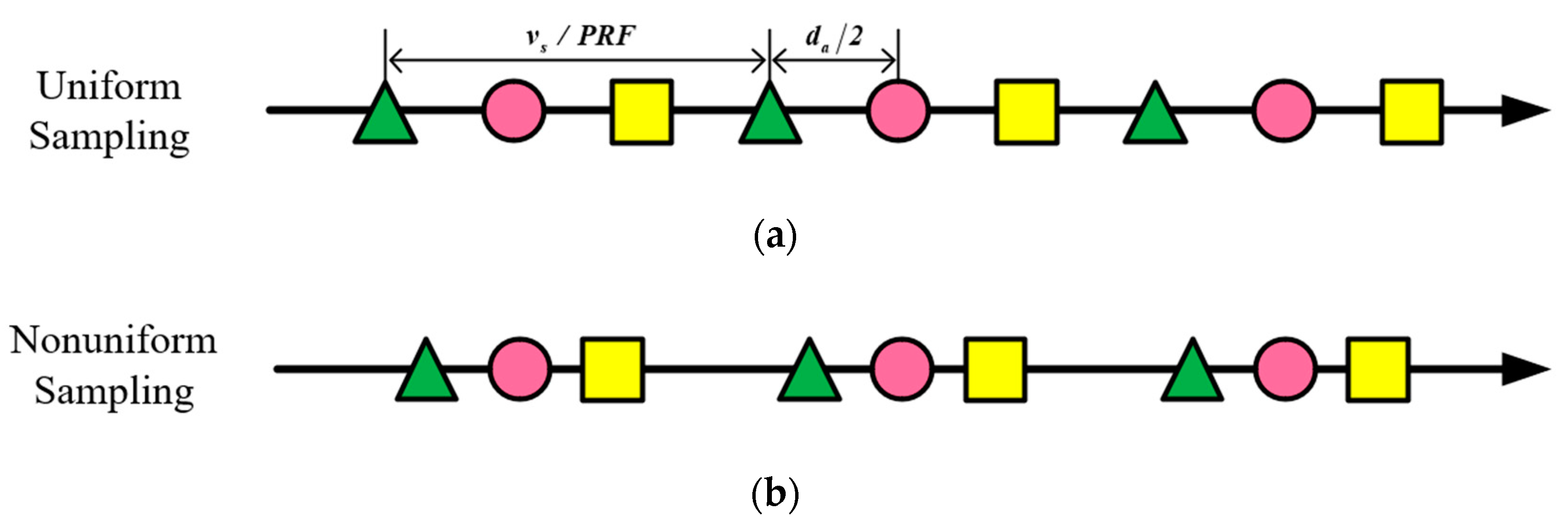
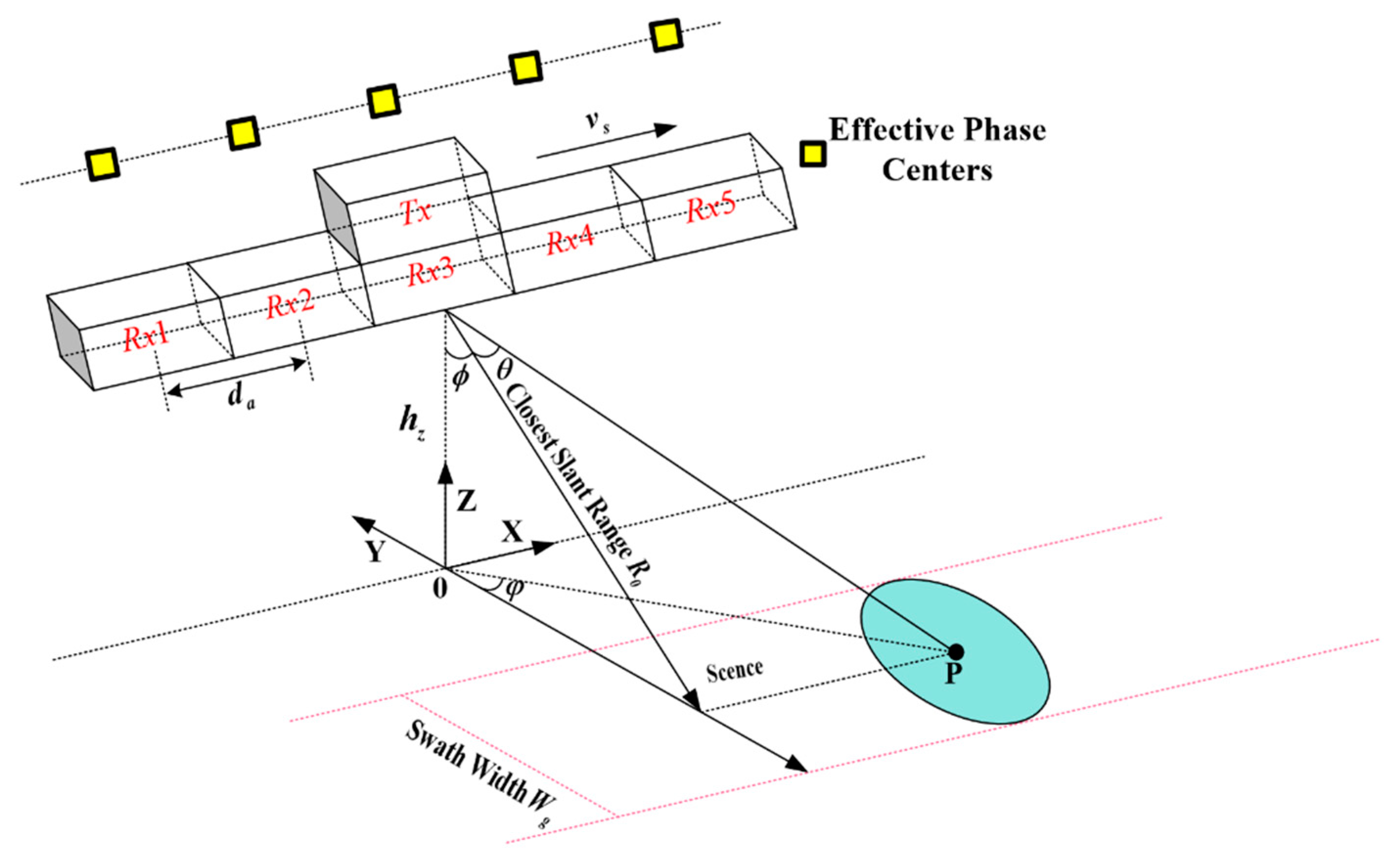
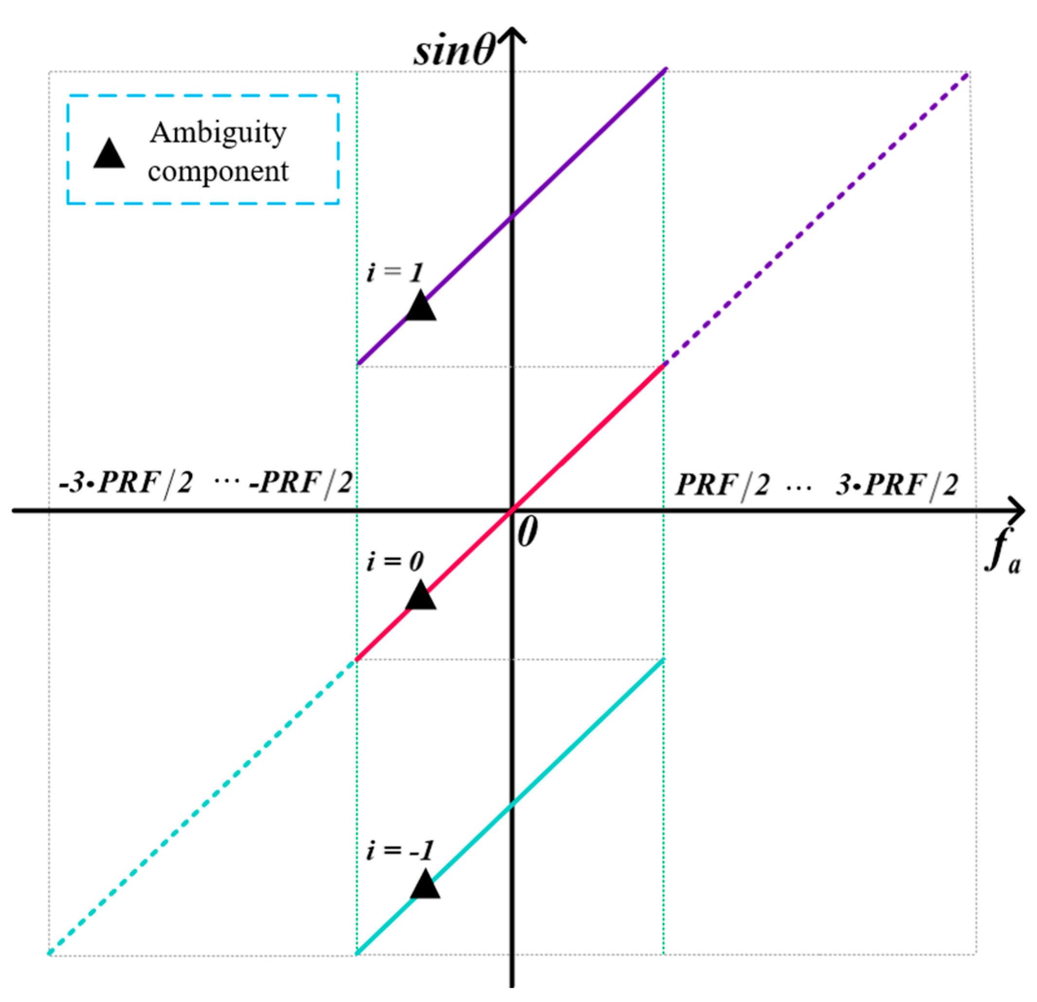
2. Signal Model
3. Related Work
3.1. The DBF Reconstruction Algorithm
3.2. The IDBF Reconstruction Algorithm
4. Proposed Approach
4.1. Problem Formulation
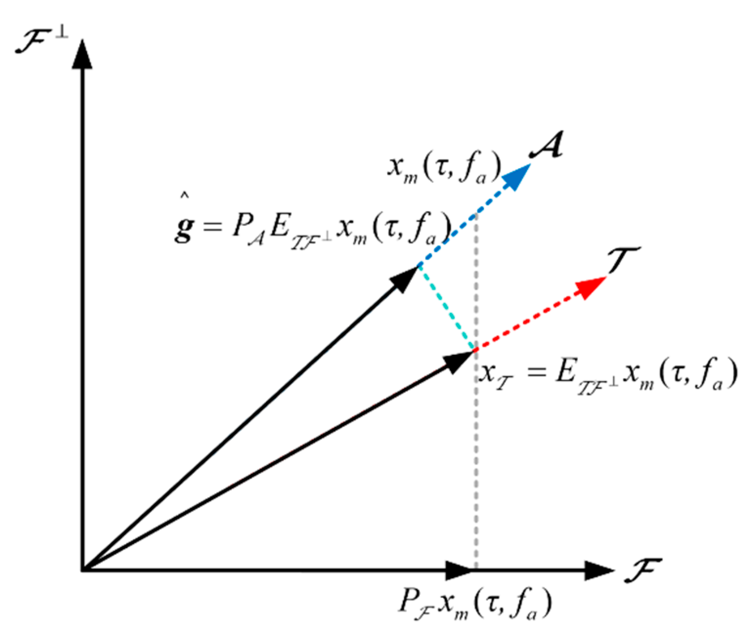
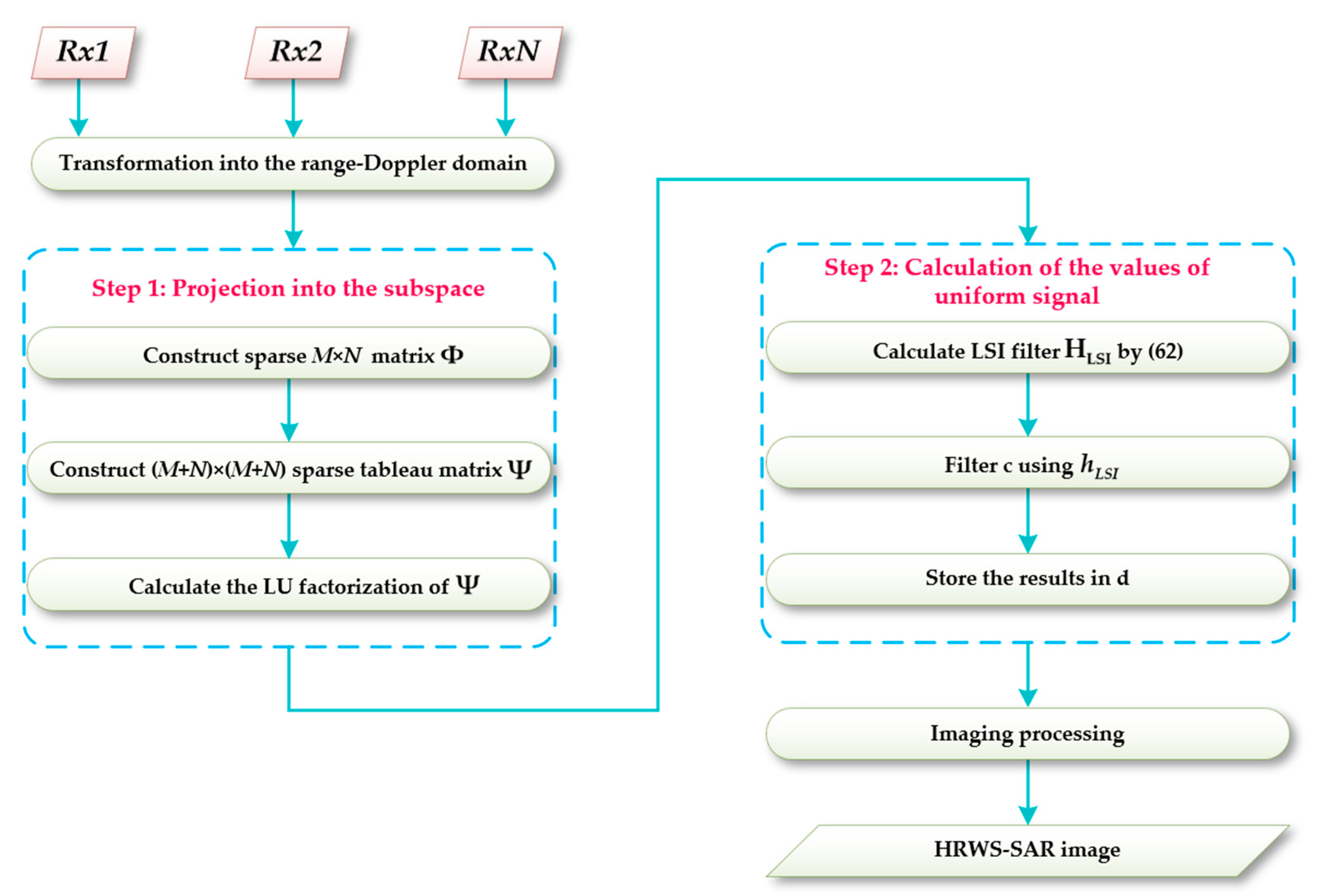
4.2. The Proposed Method
| Algorithm 1: TSPT—Preparation and Solution |
Input:
|
5. Experiment Results
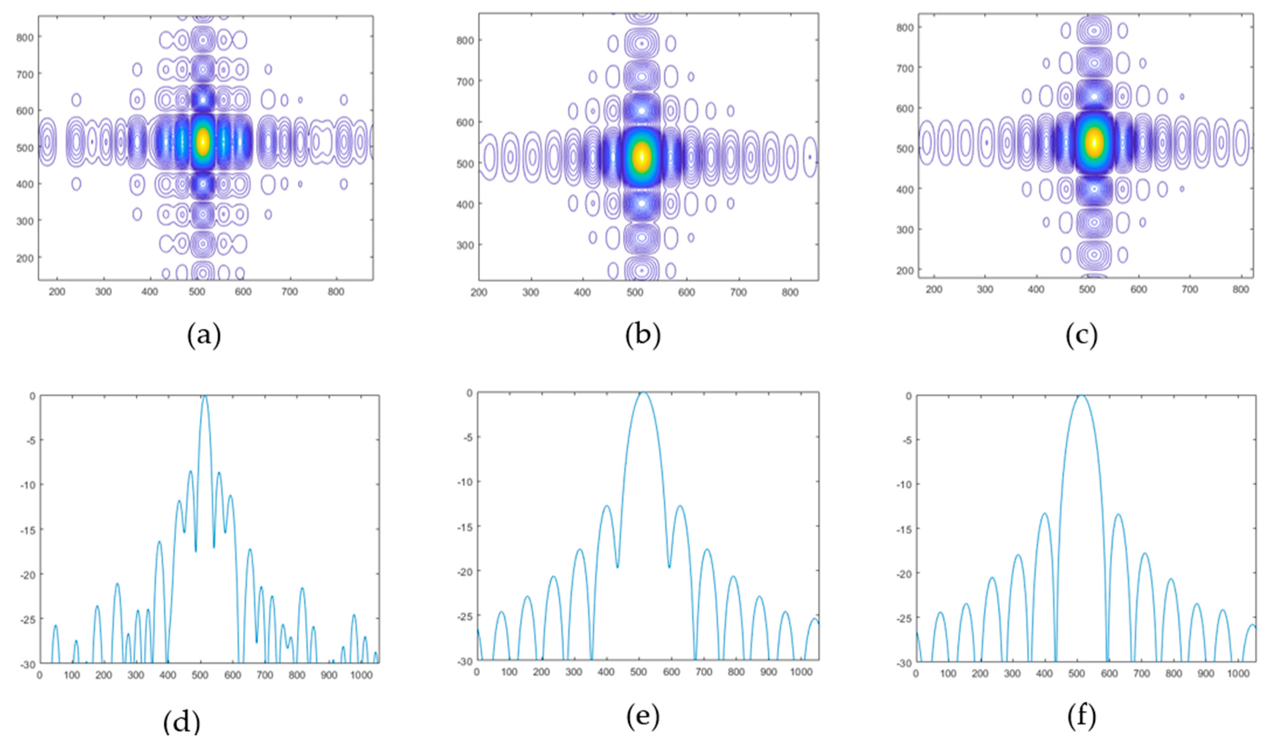
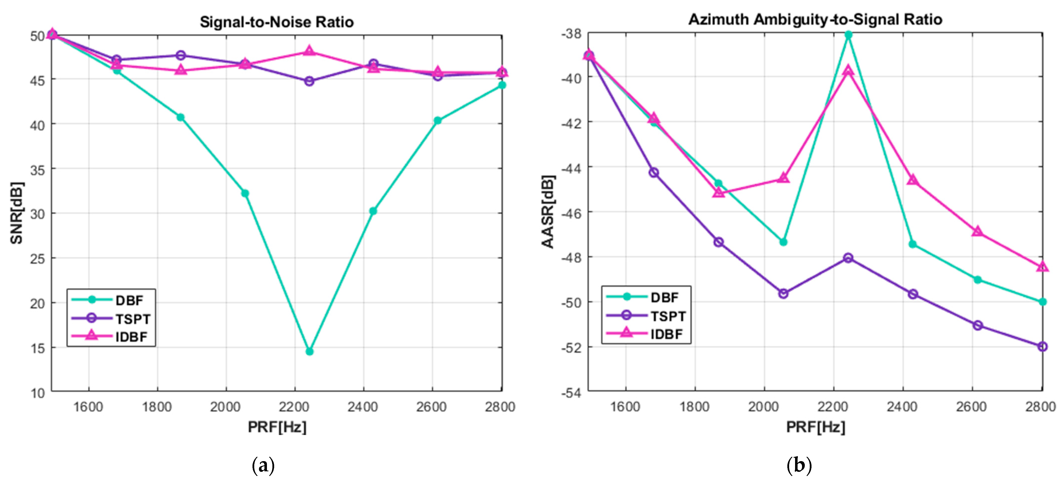
5.1. Simulation Results
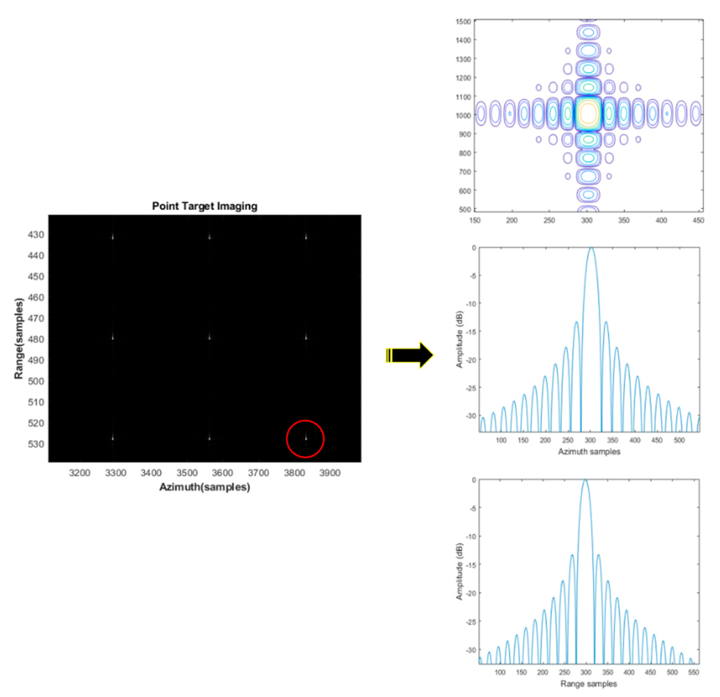
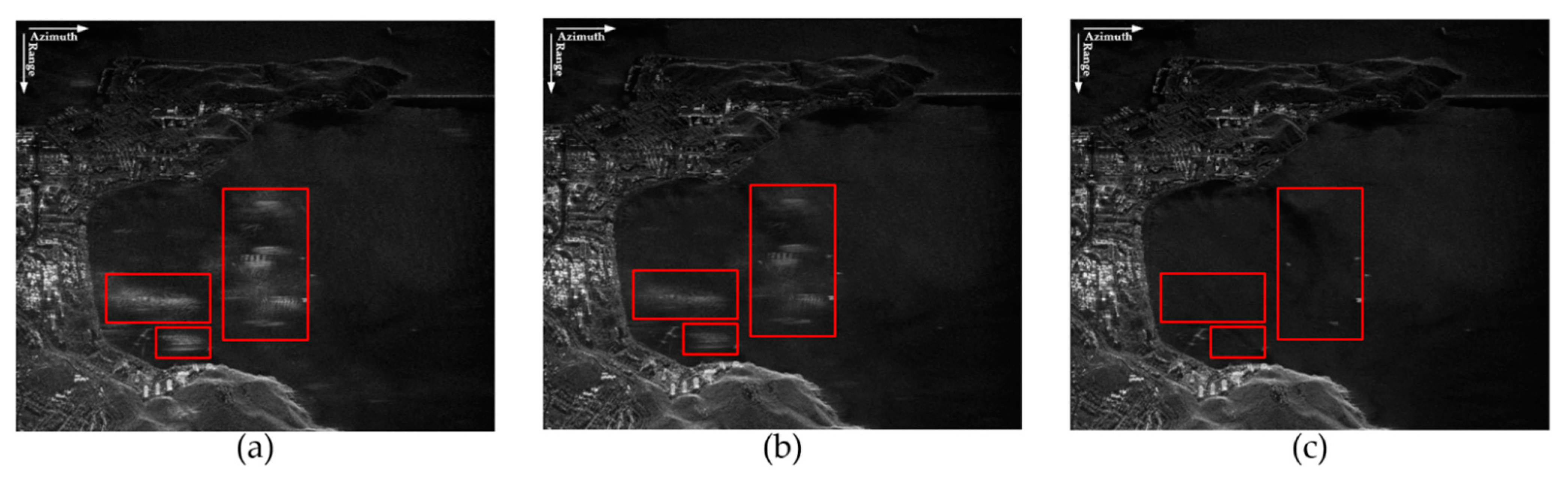
5.2. MCSAR Real Data Processing
6. Conclusions
Author Contributions
Funding
Acknowledgments
Conflicts of Interest
References
- Cumming, I.G.; Wong, F.H. Digital Processing of Synthetic Aperture Radar Data: Algorithms and Implementation; Artech House: Norwood, MA, USA, 2005. [Google Scholar]
- Villano, M.; Krieger, G.; Moreira, A. Staggered SAR: High-Resolution Wide-Swath Imaging by Continuous PRI Variation. IEEE Trans. Geosci. Remote Sens. 2014, 52, 4462–4479. [Google Scholar] [CrossRef]
- Kim, J.; Younis, M.; Prats-Iraola, P.; Gabele, M.; Krieger, G. First Spaceborne Demonstration of Digital Beamforming for Azimuth Ambiguity Suppression. IEEE Trans. Geosci. Remote Sens. 2013, 51, 579–590. [Google Scholar] [CrossRef] [Green Version]
- Yang, J.; Qiu, X.; Zhong, L.; Shang, M.; Ding, C. A Simultaneous Imaging Scheme of Stationary Clutter and Moving Targets for Maritime Scenarios with the First Chinese Dual-Channel Spaceborne SAR Sensor. Remote Sens. 2019, 11, 2275. [Google Scholar] [CrossRef] [Green Version]
- Xu, W.; Wei, Z.; Huang, P.; Tan, W.; Liu, B.; Gao, Z.; Dong, Y. Azimuth Multi-Channel Reconstruction for Moving Targets in Geosynchronous Spaceborne–Airborne Bistatic SAR. Remote Sens. 2020, 12, 1703. [Google Scholar] [CrossRef]
- Curlander, J.; McDonough, R. Synthetic Aperture Radar: Systems and Signal Processing; Artech House: Hoboken, NJ, USA, 1991. [Google Scholar]
- Gebert, N.; Almeida, F.; Krieger, G. Airborne demonstration of multichannel SAR imaging. IEEE Trans. Geosci. Remote Sens. Lett. 2011, 8, 963–967. [Google Scholar] [CrossRef]
- Freeman, A.; Johnson, W.T.K.; Huneycutt, B.; Jordan, R.; Hensley, S.; Siqueira, P.; Curlander, J. The myth of the minimum SAR antenna area constraint. IEEE Trans. Geosci. Remote Sens. 2000, 38, 320–324. [Google Scholar] [CrossRef] [Green Version]
- Krieger, G.; Gebert, N.; Moreira, A. Unambiguous SAR signal-reconstruction from nonuniform displaced phase center sampling. IEEE Geosci. Remote Sens. Lett. 2004, 1, 260–264. [Google Scholar] [CrossRef] [Green Version]
- Gebert, N.; Krieger, G.; Moreira, A. Digital Beam Forming for HRWS-SAR Imaging: System Design, Performance and Optimization Strategies. In Proceedings of the 2006 IEEE International Symposium on Geoscience and Remote Sensing, Denver, CO, USA, 31 July–4 August 2006; pp. 1836–1839. [Google Scholar] [CrossRef] [Green Version]
- Gebert, N.; Krieger, G.; Younis, M.; Bordoni, F.; Moreira, A. Ultra Wide Swath Imaging with Multi-Channel ScanSAR. In Proceedings of the IEEE International Geoscience and Remote Sensing Symposium, Boston, MA, USA, 6–11 July 2008; pp. v21–v24. [Google Scholar] [CrossRef]
- Zhang, Y.; Wang, W.; Deng, Y.; Wang, R. Signal-reconstruction Algorithm for Azimuth Multichannel SAR System Based on a Multiobjective Optimization Model. IEEE Trans. Geosci. Remote Sens. 2020, 58, 3881–3893. [Google Scholar] [CrossRef]
- Krieger, G.; Gebert, N.; Moreira, A. Multidimensional Waveform Encoding: A New Digital Beamforming Technique for Synthetic Aperture Radar Remote Sensing. IEEE Trans. Geosci. Remote Sens. 2008, 46, 31–46. [Google Scholar] [CrossRef] [Green Version]
- Gebert, N.; Krieger, G.; Moreira, A. Multi-channel Azimuth Processing in ScanSAR and TOPS Mode Operation. IEEE Trans. Geosci. Remote Sens. 2010, 48, 2994–3008. [Google Scholar] [CrossRef] [Green Version]
- Zhao, S.; Wang, R.; Deng, Y.; Zhang, Z.; Li, N.; Guo, L.; Wang, W. Modifications on Multichannel Reconstruction Algorithm for SAR Processing Based on Periodic Nonuniform Sampling Theory and Nonuniform Fast Fourier Transform. IEEE J. Sel. Top. Appl. Earth Obs. Remote Sens. 2015, 8, 4998–5006. [Google Scholar] [CrossRef]
- Younis, M.; Fischer, C.; Wiesbeck, W. Digital beamforming in SAR systems. IEEE Trans. Geosci. Remote Sens. 2003, 41, 1735–1739. [Google Scholar] [CrossRef]
- Gebert, N.; Krieger, G. Azimuth Phase Center Adaptation on Transmit for High-Resolution Wide-Swath SAR Imaging. IEEE Trans. Geosci. Remote Sens. Lett. 2009, 6, 782–786. [Google Scholar] [CrossRef]
- Currie, A.; Gebert, N.; Brown, M.A. Wide-swath SAR. IEE Proc. F Radar Signal Process. 1992, 139, 122–135. [Google Scholar] [CrossRef]
- Li, Z.; Wang, H.; Su, T.; Bao, Z. Generation of wide-swath and high-resolution SAR images from multi-channel small spaceborne SAR systems. IEEE Geosci. Remote Sens. Lett. 2005, 2, 82–86. [Google Scholar] [CrossRef]
- Li, Z.; Wang, H.; Bao, Z.; Liao, G. Performance improvement for constellation SAR using signal processing techniques. IEEE Trans. Aero. Elec. Sys. 2006, 42, 436–452. [Google Scholar] [CrossRef]
- Liu, B.; He, Y. Improved DBF Algorithm for Multi-channel High-Resolution Wide-Swath SAR. IEEE Trans. Geosci. Remote Sens. 2016, 54, 1209–1225. [Google Scholar] [CrossRef]
- Liu, N.; Wang, R.; Deng, Y.; Zhao, S.; Wang, X. Modified Multi-Channel Reconstruction Method of SAR with Highly Nonuniform Spatial Sampling. IEEE J. Sel. Top. Appl. Earth Obs. Remote Sens. 2017, 10, 617–627. [Google Scholar] [CrossRef]
- Zuo, S.; Xing, M.; Xia, X.; Sun, G. Improved Signal-reconstruction Algorithm for Multi-channel SAR Based on the Doppler Spectrum Estimation. IEEE J. Sel. Top. Appl. Earth Obs. Remote Sens. 2017, 10, 1425–1442. [Google Scholar] [CrossRef]
- Zhang, S.; Xing, M.; Xia, X.; Zhang, L.; Guo, R.; Liao, Y.; Bao, Z. Multi-channel HRWS SAR Imaging Based on Range-Variant Channel Calibration and Multi-Doppler-Direction Restriction Ambiguity Suppression. IEEE Trans. Geosci. Remote Sens. 2014, 52, 4306–4327. [Google Scholar] [CrossRef]
- Gebert, N.; Krieger, G.; Moreira, A. Digital Beamforming on Receive: Techniques and Optimization Strategies for High-Resolution Wide-Swath SAR Imaging. IEEE Trans. Aero. Electron. Sys. 2009, 45, 564–592. [Google Scholar] [CrossRef] [Green Version]
- Kiperwas, A.; Rosenfeld, D.; Eldar, Y.C. The SPURS Algorithm for Resampling an Irregularly Sampled Signal onto a Cartesian Grid. IEEE Trans. Med. Imaging 2017, 36, 628–640. [Google Scholar] [CrossRef] [PubMed]
- Zhang, L.; Gao, Y.; Wang, K.; Liu, X. A Blind Reconstruction of Azimuth Signal for Multi-Channel HRWS SAR System. In Proceedings of the Proceedings of the 2017 IEEE Radar Conference (RadarConf), Seattle, WA, USA, 8–12 May 2017; pp. 1020–1023. [Google Scholar] [CrossRef]
- Zhang, L.; Gao, Y.; Wang, K.; Liu, X. Azimuth Signal-Reconstruction for HRWS SAR from Recurrent Nonuniform Samples. In Proceedings of the 2016 CIE International Conference on Radar (RADAR), Guangzhou, China, 10–13 October 2016; pp. 1–4. [Google Scholar] [CrossRef]
- Li, Z. Distributed Small Satellite SAR-InSAR-GMTI Signal Processing Algorithms. Ph.D. Thesis, Xidian University, Xi’an, China, 2006. [Google Scholar]
- Zhang, S. High-Resolution and Wide-Swath Multi-Channel SAR and Moving Target Imaging Theory and Methods. Ph.D. Thesis, Xidian University, Xi’an, China, 2014. [Google Scholar]
- Zhang, L. Azimuth Multi-Channel High-resolution and Wide-swath SAR Imaging Processing Technique. Ph.D. Thesis, Shanghai Jiao Tong University, Shanghai, China, 2018. [Google Scholar]
- Davis, T.A.; Gao, Y.; Wang, K.; Liu, X. An unsymmetric-pattern multifrontal method. ACM Trans. Math. Softw. 2004, 30, 196–199. [Google Scholar] [CrossRef]
- Davis, T.A. Direct Methods for Sparse Linear Systems; Artech House: Philadelphia, MA, USA, 2006. [Google Scholar]
- Eldar, Y.C. Sampling Theory: Beyond Bandlimited Systems; Cambridge University Press: Cambridge, UK, 2015. [Google Scholar]
- Zhao, P.; Deng, Y.; Wang, W.; Zhang, Y.; Wang, R. Ambiguity Suppression Based on Joint Optimization for Multi-channel Hybrid and ±π/4 Quad-Pol SAR Systems. Remote Sens. 2021, 13, 1907. [Google Scholar] [CrossRef]


| Parameter | Value |
|---|---|
| Carrier Wavelength | 0.03 m |
| Doppler Band Width | 3737.4 Hz |
| Channel Number | 3 |
| Platform Velocity | 7474.8 m/s |
| Adjacent Channel Interval | 3.3333 m |
| Slant Range | 890 km |
| Uniform PRF | 1495 Hz |
| Parameter | Value |
|---|---|
| Carrier Frequency | 1.3 GHz |
| PRF | 149.92 Hz |
| Channel Number | 2 |
| Platform Velocity | 129.8 m/s |
| Adjacent Channel Interval | 0.86 m |
| Slant Range | 1.58 km |
| Azimuth Band Width | 190.91 Hz |
| Range Band Width | 210 MHz |
| Range Sampling Rate | 266 MHz |
| Antenna Length | 1.36 m |
Publisher’s Note: MDPI stays neutral with regard to jurisdictional claims in published maps and institutional affiliations. |
© 2021 by the authors. Licensee MDPI, Basel, Switzerland. This article is an open access article distributed under the terms and conditions of the Creative Commons Attribution (CC BY) license (https://creativecommons.org/licenses/by/4.0/).
Share and Cite
Li, N.; Zhang, H.; Zhao, J.; Wu, L.; Guo, Z. An Azimuth Signal-Reconstruction Method Based on Two-Step Projection Technology for Spaceborne Azimuth Multi-Channel High-Resolution and Wide-Swath SAR. Remote Sens. 2021, 13, 4988. https://doi.org/10.3390/rs13244988
Li N, Zhang H, Zhao J, Wu L, Guo Z. An Azimuth Signal-Reconstruction Method Based on Two-Step Projection Technology for Spaceborne Azimuth Multi-Channel High-Resolution and Wide-Swath SAR. Remote Sensing. 2021; 13(24):4988. https://doi.org/10.3390/rs13244988
Chicago/Turabian StyleLi, Ning, Hanqing Zhang, Jianhui Zhao, Lin Wu, and Zhengwei Guo. 2021. "An Azimuth Signal-Reconstruction Method Based on Two-Step Projection Technology for Spaceborne Azimuth Multi-Channel High-Resolution and Wide-Swath SAR" Remote Sensing 13, no. 24: 4988. https://doi.org/10.3390/rs13244988