Article

Radar Imaging Statistics of Non-Gaussian Rough Surface: A Physics-Based Simulation Study

1
School of Information Engineering, Xuchang University, Xuchang 461002, China
2
College of Geomatics and Geoinformation, Guilin University of Technology, Guilin 541004, China
3
School of Electronic and Optical Engineering, Nanjing University of Science and Technology, Nanjing 210094, China
*
Author to whom correspondence should be addressed.
Remote Sens. 2022, 14(2), 311; https://doi.org/10.3390/rs14020311
Submission received: 18 November 2021 / Revised: 21 December 2021 / Accepted: 29 December 2021 / Published: 11 January 2022
(This article belongs to the Special Issue Radar Imaging Theory, Techniques, and Applications II)

Abstract

:
This paper investigates the radar image statistics of rough surfaces by simulating the scattered signal’s dependence on the surface roughness. Statistically, the roughness characteristics include the height probability density (HPD) and, to the second-order, the power spectral density (PSD). We simulated the radar backscattered signal by computing the far-field scattered field from the rough surface within the antenna beam volume in the context of synthetic aperture radar (SAR) imaging. To account for the non-Gaussian height distribution, we consider microscopic details of the roughness on comparable radar wavelength scales to include specularly, singly, and multiply scatterers. We introduce surface roughness index (RSI) to distinguish the statistical characteristics of rough surfaces with different height distributions. Results suggest that increasing the RMS height does not impact the Gaussian HPD surface but significantly affects the Weibull surface. The results confirm that as the radar frequency increases, or reaches a relatively larger roughness, the surface’s HPD causes significant changes in incoherent scattering due to more frequent multiple scattering contributions. As a result, the speckle move further away from the Rayleigh model. By examining individual RSI, we see that the Gaussian HPD surface is much less sensitive to RMS height than the Weibull HPD surface. We demonstrate that to retrieve the surface parameters (both dielectric and roughness) from the estimated RCS, less accuracy is expected for the non-Gaussian surface than the Gaussian surface under the same conditions. Therefore, results drawn from this study are helpful for system performance evaluations, parameters estimation, and target detection for SAR imaging of a rough surface.

1. Introduction

Understanding the speckle properties is imperative for both image de-noising and remote sensing applications. Radar speckle arises due to the sum of numerous distributed scattering contributions. Given previous studies, progress of understanding the image statistics of rough surfaces has been made in both depth and breadth scopes. The randomly rough surface is a stochastic random process, and it is in multiscale nature. The presence of many scales of roughness is termed “fractal” [1]. It has been argued that the fractal dimension is a vital parameter to characterize the rough surface [2]. Without accounting for the multiscale roughness effect, the backscattering strength was overestimated to 2–3 dB compared to field measurements by SAR [3]. It is known for a multiscale rough surface that depend strongly on the measuring resolution, surface height, and correlation length [4]. Roughness scales responsible for radar scattering are usually quantitatively characterized using the correlation function and the surface RMS height.
However, the subject remains complex and needs to be explored under various scenarios within the context of rough-surface scattering and imaging. Hence, a large body of work has addressed the radar speckle of imaged rough surfaces [5,6,7,8,9,10,11,12,13,14,15,16,17]. It is well known that the statistical properties of non-Gaussian speckle composed from a small number of scattering elements depends on the scattering surface’s detailed structure. Ouchi et al. [6] presented a physical model for the speckle in synthetic aperture radar (SAR) images to highlight the dependence of the speckle characteristics on the surface roughness and the sensor parameters. However, the speckle correlation function derived from the radar image of the rough surface involves no surface statistics. Yueh et al. [7] showed that the polarimetric scattering data follows a K-distribution if the number of scatterers within the antenna footprint has a negative binomial distribution.
Both perfectly spatial and temporal coherences have not been achieved in practice due to a limited aperture size and cell resolution. The research presented in [8] investigated radar backscattering and its speckle statistic variation with the resolution cell size or antenna footprint using a numerical simulation of scattering from a one-dimensional rough surface. The experimental study reported in [9] found that with a spatial resolutions in the SAR image of smaller than two correlation lengths, the statistics of the backscattered signal depended on the resolution cell size. For larger resolution cells, the speckle was consistent with the Rayleigh model. Using the first-order Kirchhoff scattering model of the fractal surface, the authors of [10] presented speckle statistics, for considerable RMS height, with Gaussian height distribution. di Martino et al. [11,12] simulated both exponentially and K-distributed speckle statistics to evaluate the equivalent number of scatterers per resolution cell, from within which the radar returns are the coherent sum of contributions from each scatterer. Chen et al. [13] performed random rough surface scattering simulations using a 3-D numerical solution of Maxwell equations (NMM3D) using a surface size of up to 32 × 32 squared wavelengths. The rough surfaces were characterized by exponential correlation functions and Gaussian height distribution. Using the ensemble of simulated scattering matrices, they calculated and examined the polarimetric speckle statistics (amplitude and phase difference). It was confirmed that the simulated data fully agreed with theoretical Wishart distributions for homogeneous rough surfaces. Di Martino et al. [14] proposed a predictive model for the equivalent number of scatterers within the resolution cell to characterize high-resolution speckle properties from the fractal surface. It was found in [15] that if the equivalent number of scatterers is not sufficiently large, the two-scale multiplicative scattering process may drive the VHR speckle PDF away from the fully developed Rayleigh distribution. Additionally, the dominance of a sufficiently sizeable equivalent number of scatterers is observed, leading the VHR speckle properties close to the fully developed model even when the resolution cell size is smaller than the correlation length. The research in [16] reported the speckle dependence on the ocean wind field, where a sensitivity of the K-distribution shape parameter on the incidence angle and wind direction is also observed. The work in [17] presented the excellent treatment of a noncentral and non-Gaussian probability model for SAR data, in which a general compound statistical model for coherent imaging was developed and tested on single-channel data by accounting for coherent scattering and modeling the texture as an inverse Gaussian distribution.
Compared to the Gaussian surface, scattering from a non-Gaussian rough surface has been studied to a much lesser extent. Furthermore, past radar image statistics studies mainly focused on Gaussian height distribution. However, in many cases, a randomly rough surface, natural or engineered, is frequently considered as a non-Gaussian process. The randomly rough surface is a stochastic process. Hence, two rough surfaces can have the same correlation function but different height distributions or vice versa [18]. The ocean surface is perhaps one of the most distinctive non-Gaussian surfaces [19]. Sea ice, which is a terrestrial surface, presented negative exponential height distribution [20]. The scattering characteristics for non-Gaussian surfaces have been investigated analytically by the Kirchhoff model, a first-order approximation, by Beckmann [21], Brown [22], Eom and Fung [23], and numerically simulation in [24]. When the surface approaches the region of the geometric optic due to the high-frequency limit, the convergent rate is found to be slower for non-Gaussian than Gaussian surfaces. The non-Gaussian height distributed rough surface generally causes higher coherent scattering for the same roughness parameters. Additionally, the polarization dependences are different between Gaussian and non-Gaussian surfaces. Hence, it is of particular interest to examine the effect of non-Gaussian height distribution on the radar image statistics, the main objective of this study.

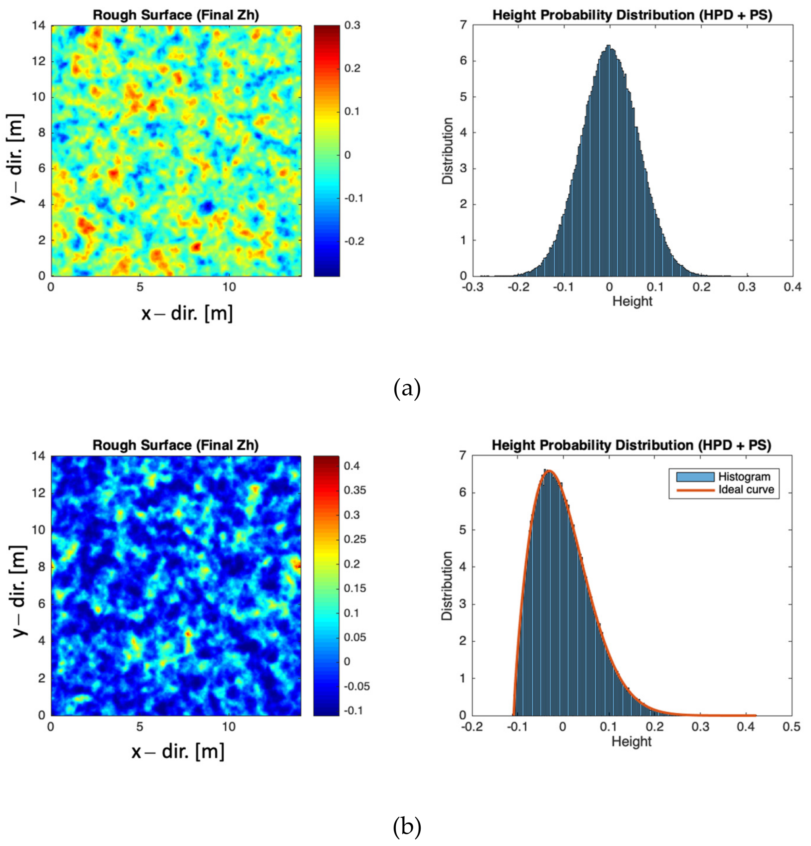
2. Generating Non-Gaussian Rough Surface

2.1. Roguh Surface Parameters

We consider a Non-Gaussian height distribution. Following the algorithm proposed in [25], we generated many ensemble samples of the statistically specified rough surface. Special care should be taken to generate rough surfaces to ensure the purity of the statistics. We generated a rough surface with roughness parameters, the RMS height, and correlation length. Two more important settings are the height probability density (HPD) and power spectral density (PSD) (or equivalently, a correlation function). Note that the generated rough surface does not precisely match the HPD and PSD for the finite size of the surface. The error for either one is practically negligible. It has been argued in [26] that the appropriate choice of surface and statistically representative grid sizes pose a problematic issue. An entropy measurement was applied to determine such parameter settings by examining the relative error of sample entropy associated with roughness parameters and noticing that a rough surface with specific roughness parameters, including power spectrum density function, must have unique sample entropy. It is found that if the two criteria are met, the suitable choice of surface length and grid size is attainable to allow for minimum uncertainties of rough surfaces and maximum information content for different roughness spectra density functions under different correlation lengths.
For this study, we consider both Gaussian and Weibull HPDs, Gaussian and exponential PSDs. We selected the Weibull HPD because of its wide application. As discussed in [27], the Weibull distribution, which is inherently asymmetric, can be used for a more accurate representation of surfaces that may not be amenable by Gaussian distribution. Mathematically, the Weibull HPD is expressed by
p ( z ) = κ ν ( z z 0 ) ν κ 1 e [ ( z z 0 ) / ν ] κ , ( z z 0 ) 0
where υ , κ are the shape and scale parameters, respectively; z 0 is the location parameter. From (1), the HPD approaches the exponential and Rayleigh, respectively, when κ 1 , and κ 2 . The correlation function is an essential statistical property. For the natural surface, we considered the exponential correlation function to be bandlimited. The PSD is related to the correlation function as demonstrated by the Wiener-Khinchin theorem. The exponential PSD is of the form by using normalized Fourier transform:
S e K = s 2 2 1 + K 2 2 3 / 2
where K = ( K x , K y ) is spatial wavenumber vector with K x , K y the wavenumber components in x and y directions; s is the RMS height and is the correlation length, both in unit of radar wavelength. For the surface RMS height to be s , the shape parameter and scaling parameters in Equation (2) are related by
ν = s 1 Γ ( 1 + 2 / κ ) + Γ 2 ( 1 + 1 / κ )
It is worth mentioning that in the context of radar wave scattering, the rough surface is highly frequency-selective [28]. Equivalently, the PSD is bandlimited:
s 2 = K 2 π sin θ i / λ S e ( K ) d K
where λ is the radar wavelength and θ i is incident angle. The bandlimited is because spectral components of the rough surface whose spatial wavenumber is greater than 2 π / λ will produce evanescent waves and not contribute to surface scatter [29].

2.2. Surface Dimensions and Sampling Consideration

Statistically, the correlation length typically depends on the measured surface length L, and a sizeable measured surface length L yields high accuracy in estimating and measuring the correlation length. In the computer generation of random rough surfaces, the choice of surface length should guarantee a minimum error in calculating the prespecified correlation length [30]. For radar imaging statistics, we generated ensemble samples and stored each set of roughness parameters ( σ , , HPD, PSD). For a digitized surface to be representative within the radar probing wavelength, the lower limit of the sampling frequency of the surface must meet the following Nyquist sampling criteria:
f s > 2
The minimum sampling frequency confines the correlation length from the above relation. Then, the total number of the samplings along x and y-directions of the surface is:
N x = f s L x ,   N y = f s L y
where Lx × Ly is the surface size.
In addition, there is a statistical limitation on the number of statistical populations. The ratio of surface size to the correlation length should be sufficiently large so that the surface of that size preserves statistical significance:
L x , L x > M
where M is a large number, and according to [26,30], we set M to 70 to ensure the sufficiency.
To verify the statistical characteristics of the simulated surfaces, we summarized the rough surface parameters from the generated surfaces, including the RMS height and the correlation length in both directions. The results are provided in Table 1, where the data in each row is the average value generated by 20 ensemble samples. We see that the error of RMS height was well below 0.1%, and the error in correlation length is less than 2.0% for both x- and y-directions. We confirm the surfaces generated all satisfactorily met the statistics specifications, allowing us to proceed to the next step.
Figure 1 displays an ensemble sample of rough surfaces with Gaussian and Weibull HPDs, where the RMS height is 2λ, and the correlation length is 5λ; the shape parameter is 1.8. The correlation function is exponential. By visually comparing the two rough surfaces, we may find that the Weibull HPD surface presents more substantial and dramatic fluctuations in height and is not symmetric in terms of its zero-mean, producing a sharper contrast. Hence, even under the same PSD, the height distribution affects the scattering and diffraction patterns in the context of coherent radar imaging of collective surface scatterers. Therefore, to predict the image statistics more accurately, we must consider both HPD and PSD properties in the scattering process. Recalling that HPD is of first-order effect, while PSD is of higher-order effect.
The following surface parameters for SAR image simulation, generate 200 ensemble samples for each parameter set and after careful setting according to the above constraints, as listed in Table 2. Note that all parameters are units in wavelength λ .

3. SAR Echo Simulations

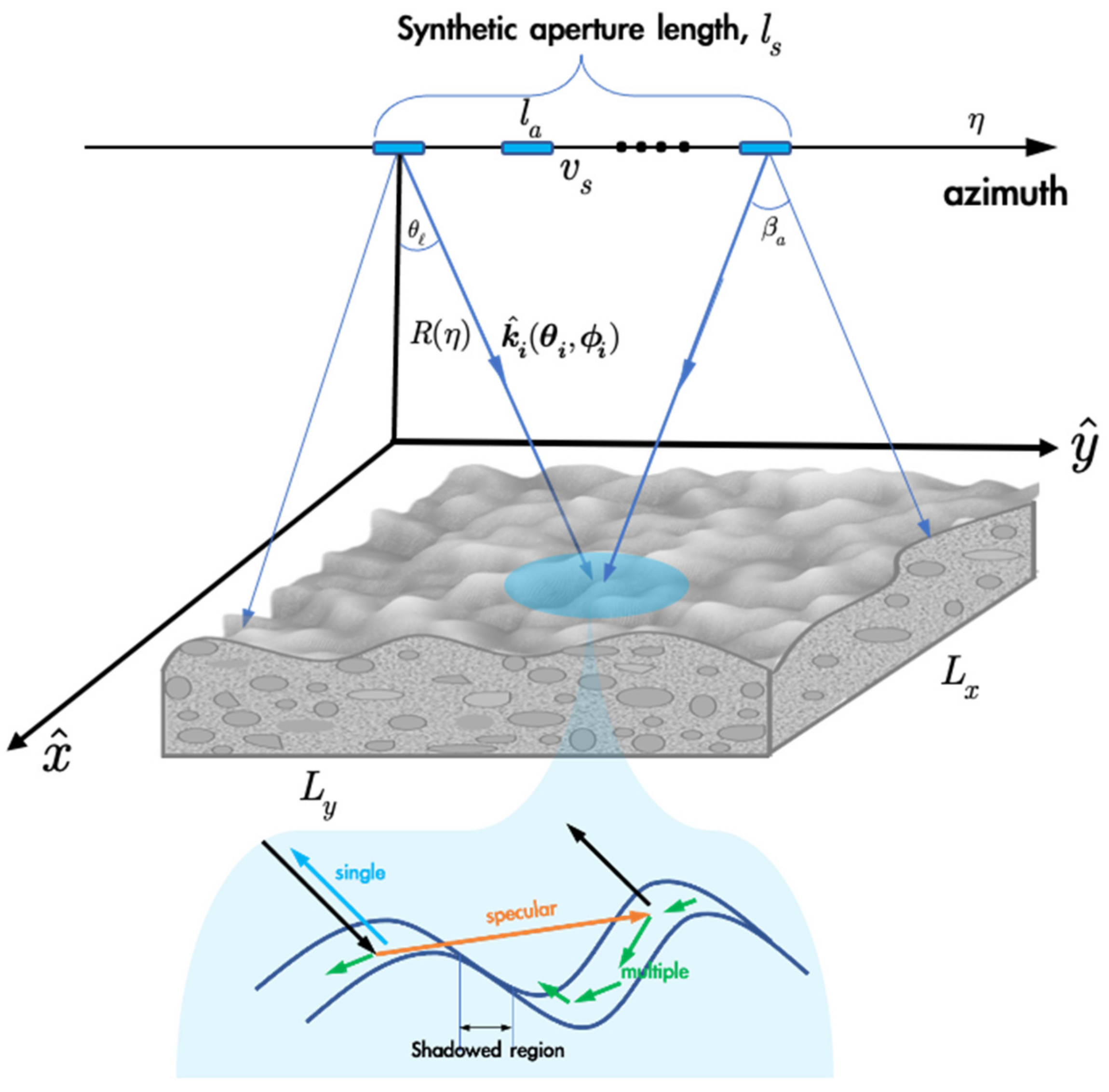
3.1. Observation Geometry and Radar Parameters

For convenience, we chose 1.27 GHz (L-band) as the radar carrier frequency. The surface size and the relevant parameters are all denoted in terms of wavelengths. Table 3 lists the major SAR simulation parameters, including the center frequency, chirp bandwidth, sampling rate, pulse width, pulse repetition frequency. We include the state vector to construct the platform path trajectory. Additionally, the look and squint angle in the SAR geometry observation is specified.
Figure 2 illustrates a SAR geometric observation over a rough surface with size L x × L y . In the figure, l s is the synthetic aperture length; l a is the real antenna length along azimuth, the SAR moving direction with velocity v s . The slant range, R ( η ) , is a function of slow time η . The radar transmits wave toward the rough surface along with the incident wavevector k ^ i ( θ i , ϕ i ) , where θ i is incident angle defined as the angle between the mean surface and the z-axis; ϕ i is the incident azimuthal angle; θ denotes the look angle. Within the course of aperture synthesis, the radar continuously illuminates a resolution cell and then coherently sums up the scattered fields within the beamwidth of the synthetic aperture, as raw data to be processed. In such a process, the illumination direction varies within the beamwidth of the real aperture, β a , for a given resolution cell. Hence, tracking the antenna angle in the context of synthetic radar scattering is necessary so as to account for the angular variations. For backscattering, the scattering azimuth angle is ϕ i + π . As illustrated in Figure 2, once the incident wave impinges upon the rough surface, specularly, singly, and multiply scattering waves are generated, depending on the surface roughness. The specular scattering is coherent, while the single and multiple scattering are diffuse. The details of calculating the scattered field are provided in the following subsection.
Given the geometric surface structures shown in Figure 3, the single scattering and local tangent-plane approximations may no longer be valid or even broken down. As illustrated in Figure 4, during aperture synthesis, the received signal is a superposition of waveforms produced by several scatterers distributed randomly over the synthetic aperture footprint. Each of these waveforms has a time delay and Doppler shift. Hence, it is imperative to collect all the backscattered fields within the beam volume of the synthetic aperture along the azimuthal direction under the “stop-and-go” model [31]. Figure 5 depicts the coherent signal transmission and reception from a rough surface.

3.2. SAR Signal Model

The SAR echo signal in the time domain results from the collective scattered fields E q p s τ , η , also called the reflectivity field, convolving with the radar system impulse response, point spread function, P S F τ τ , η , and is mathematically expressed as, assuming a pulse radar:
S 0 τ , η = E q p s τ , η 2 d P S F τ τ , η = E s τ , η 2 d p r τ 2 R η c g a η η c . exp j 4 π f c R η c exp j π a r τ 2 R η c 2
In Equation (8), 2 d denotes a two-dimensional convolution operator; q, p denote the transmitting and receiving polarizations. The convolution operation becomes a multiplication for the point target model or ideal resolution [32]. For a non-ideal resolution system and extended target model, the convolution affects the imaged target resolution, fuzziness, and contrast [32]. We may express Equation (1) in the frequency domain as follows:
S 0 f τ , η = E ˜ q p s f τ , η × P S F f τ f τ , η = E ˜ q p s f τ , η × P r f τ g a η η c × exp j 4 π f c + f τ R η c exp j π f τ 2 a r
where τ , η denotes the fast time and slow time; c is the speed of light; R ( η ) is the SAR range to the center of footprint and varies with the slow time; p r ( ) is the envelop function for fast time domain; a r is the chirp rate, f c is the carrier frequency; R 0 is the shortest distance.
We apply the mesh generation [33] to discrete the randomly rough surfaces generated in Section 2 for numerical simulation. The number of patches is determined by the target’s geometry complexity and electromagnetic size. We digitized the rough surface in a sampling density following at least 15 samples per radar wavelength [34]. Although several grid generation algorithms and mesh formats exist, we adopted the 3ds algorithm [35] with triangular patches. Each triangular patch was appropriately oriented and positioned based on Earth Centered Rotating (ECR) coordinates [31] to realize the imaging scenario.

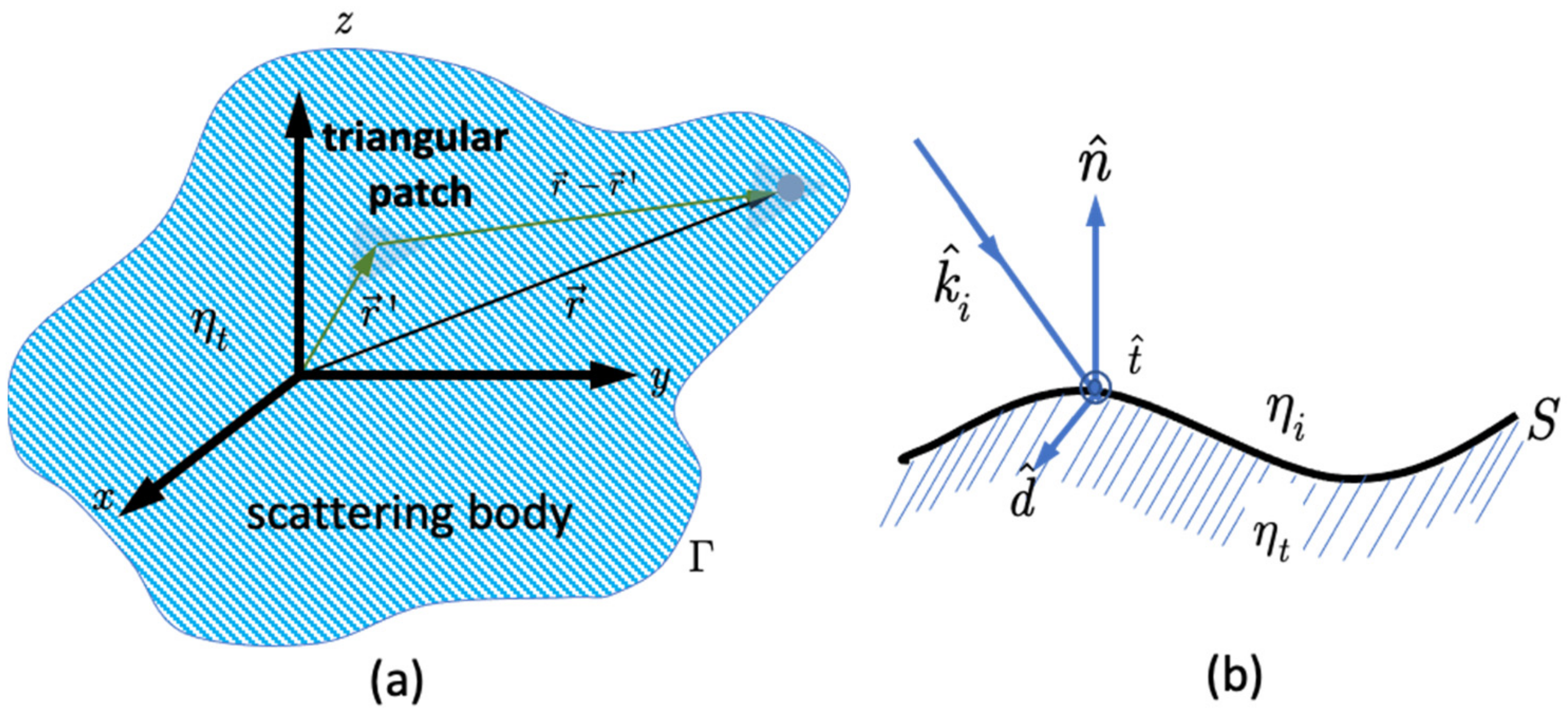
3.3. Computing the SAR Backscattered Field by an Improved Kirchhoff Method

Numerous fast computation algorithms have been proposed to solve the scattered field in the frequency domain or time domain [36,37]. Although the solutions may be accurate, they are still computationally prohibitive for an electrically large and complex target for SAR image simulation. As we already saw from Equation (8), the scattered field must be collectively calculated when SAR moves because the incident wave direction changes within the antenna beamwidth at the azimuthal direction. If we further consider the target orientation or the randomly rough surface, for which many ensemble samples are required, to build an SAR image database, the computation of the scattered fields would stall, if not stop, the simulation.
When an incident field impinges upon the rough surface, the surface fields, including the surface electric current density J s and magnetic current density M s are induced; here, we ignored the diffraction field for a moment. The near-field scattering over a triangular patch of the rough surface is shown in Figure 3a. However, the determination of the surface field over a rough surface is very complex. Mathematically, we were required to solve the electric field integral equation (EFIE) and the magnetic field integral equation (MFIE) governing the surface current densities excitation by the incident field upon the surface. Instead of solving the equations by matrix methods, we adopted the iterative scheme.
We defined a local tangent plane on which the incident field is decomposed in accordance with a local coordinate system (see Figure 3b).
t ^ = k ^ i × n ^ k ^ i × n ^ , d ^ = k ^ i × t ^ , k ^ i = t ^ × d ^
where n ^ is unit normal vector pointing out of surface. We may decompose the incident field into t ^ and d ^ components, forming the Kirchhoff surface fields:
J k = ( 1 R v ) ( n ^ × d ^ ) ( d ^ E i ) + ( 1 + R h ) ( n ^ × t ^ ) ( t E i )
M k = ( 1 + R v ) ( n ^ × t ^ ) ( t ^ H i ) + ( 1 R h ) ( n ^ × d ^ ) ( d ^ H i )
where R v , R h are Fresnel reflection coefficients for vertical and horizontal polarizations, respectively.
Note that the Kirchhoff approximation assumes the incident and reflected waves to be coplanar. Hence, the Fresnel reflection coefficients are evaluated at a local incidence. However, the Kirchhoff approximation does not account for the field in the shadow region. It is well-known that the Kirchhoff fields, as given in below, are a good initial guess to start with [38,39]. The surface integral equations suitable for iteration were developed in [39] to correct a drawback of using the standard pair of integral equations for a dielectric surface boundary resulting in a non-vanished tangential electric field on a perfectly conducting surface, thus generating errors for surfaces with moderately large dielectric values. The new pair of integral equations is as follows [39]:
J s = J k + 1 4 π ( n ^ × t ^ ) ( n ^ × t ^ ) n ^ × L e 1 [ J s , M s ] 1 4 π t ^ t ^ n ^ × L e 2 [ J s , M s ]
M s = M k + 1 4 π ( n ^ × t ^ ) ( n ^ × t ^ ) n ^ × L h 1 [ J s , M s ] + 1 4 π t ^ t ^ n ^ × L h 2 [ J s , M s ]
where the operators are defined as:
L e 1 [ J s , M s ] = Γ ( 1 + R h ) E i + ( 1 R h ) E t d s
L e 2 [ J s , M s ] = Γ ( 1 R v ) E i + ( 1 + R v ) E t d s
L h 2 [ J s , M s ] = Γ ( 1 R h ) H i + ( 1 R v ) H t d s
L h 1 [ J s , M s ] = Γ ( 1 + R v ) H i + ( 1 R v ) H t d s
These operators act on the surface of the target or a rough surface. The Fresnel reflection coefficients are locally evaluated as they appear inside the integrals. The field quantities inside the integrals of Equations (15)–(18) are given by:
E i = j k i η i M s G i J s × G i j η i k i ( s M s ) G i
E t = [ j k t η t M s G t J s × G t j η i ε r k i ( s M s ) G t
H i = j k i η i J s G + M s × G i j 1 k i η i ( s J s ) G i
H t = j k t η t J s G t + M s × G t j 1 k i η i μ r ( s J s ) G t
where s is a surface divergence operator. The surface divergence of the currents s J s , s M s physically involve the surface charge density. The above quantities account for the near-field interactions. The Green’s functions for the incident medium and transmitted medium are:
G i = exp { j k i | r r | } / [ 4 π | r r | ] G t = exp { j k t | r r | } / [ 4 π | r r | ]
Equations (13) and (14) constitute the Fredholm integral equation of the second kind, which may be solved using an iterative approach. To begin with the iterative solution, we substitute the Kirchhoff fields into Equations (15)–(18). The integral terms, called the complementary fields, are corrections to the Kirchhoff fields J k , M k . When the scattering body, becomes electrically very large, the integral terms are negligibly small, and the high-frequency approximation of Kirchhoff fields is sufficiently accurate. The iterative procedure can be continued until convergence is reached. We exclude the edges diffraction by computing the integrals of (15)–(18), which are considered later. Additionally, we applied the shoot-bouncing-ray (SBR) technique [31,32] to enhance the propagation path tracking efficiency in computing. Once the surface current densities are estimated, the scattered field can be calculated by the Stratton-Chu formula.
E I K r , θ , ϕ = j k i 4 π R e j k i R A [ η i J s + k ^ s × M s ] e j k i | R | d S
where A is the illuminated area within the SAR footprint moving along the azimuthal direction; η 0 is the intrinsic impedance; | R | is the project length from r to r .

3.4. Including Diffraction Fields

The above calculation of the scattered field does not include the diffraction fields due to the edge, wedges, and other discontinuities. We use the physical theory of diffraction (PTD) to obtain the diffraction field produced by the fringe current at or near edges. The diffraction currents on the dielectric edges are given by [40]:
I e = 2 j δ ^ ( δ ^ E i ) k η 0 sin 2 γ R v f ( δ )
I m = 2 η 0 j δ ^ ( t δ ^ H i ) k sin 2 γ R h g ( δ )
where δ ^ is the unit vector tangent to the edge; γ is the angle between the edge and the incident or diffracted direction, δ is the angle between the incident direction and the top surface of the wedge, R v and R h are the corrections for the reflection coefficients of the surfaces that form the wedge given in [41] and f , g are the Ufimtsev’s diffraction coefficients for the Keller’s cone case [41]. The diffracted field due to the diffracted currents in Equations (25) and (26) are given by
E d = × × η i j k i C I e e j k i s 4 π s d + × C I m e j k i s 4 π s d
where s is the distance from an element on the contour C to the observation point; d is the differential length along the edge discontinuity length C .
The diffracted field E d is complementary to E s I K such that the total scattered field is
E s ( r , θ , ϕ ) = E I K ( r , θ , ϕ ) + E d ( r , θ , ϕ )
Computations of E s = E s I K + E d continue as SAR moves to image the targets during the aperture time, as geometrically explained in Figure 1. It is evident that the calculation of scattered fields is computationally expensive for a SAR acquisition. Furthermore, the raw signal is generated by Equation (8) for each step of receiving the scattered fields.

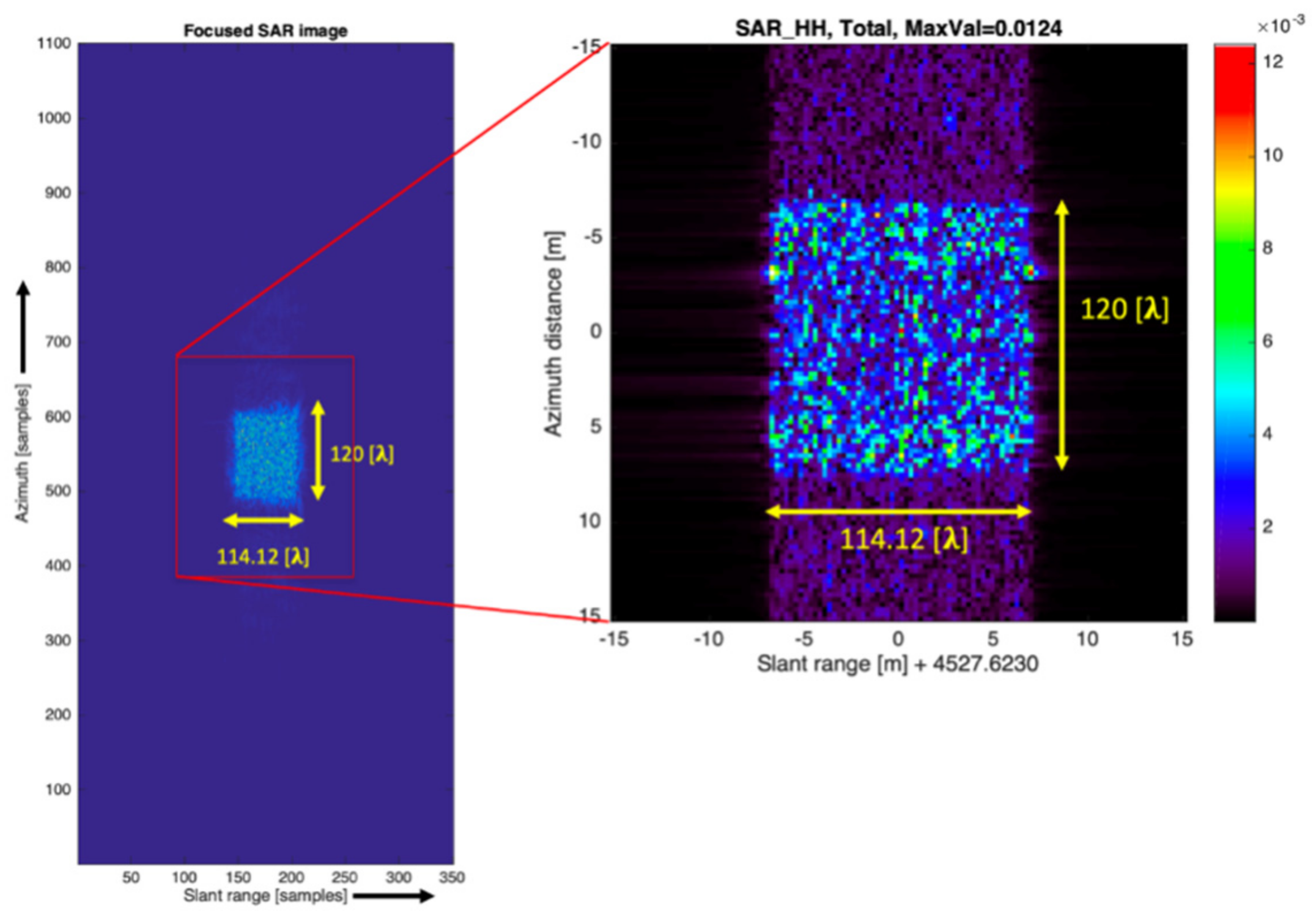
3.5. SAR Image Focusing

After the SAR data acquisition, major parameters such as exposure time, Doppler rate and bandwidth, resolution, and spacing at slant range and azimuth were derived as shown in Table 4. Following the Range-Doppler focusing algorithm [42], a single-look complex (SLC) image is formed from the SAR signal data (raw data, i.e., Equations (8) or (9)).
Figure 4 displays a sample amplitude image. The image is at the slant range; this length will be shorter than the ground range by half the squared sine of the incident angle. In the experiment, 1100 sampling points at azimuth ensured a complete synthetic aperture exposure within the surface size region. As is shown, the focused image clearly distinguishes the edge of the surface. The scattered signal strength is considered a relative value before the absolute radiometric correction.
With the above processing procedure, we generate samples of SLC SAR images to examine the image statistics. A total of five roughness were included, as given in Table 2. For illustrative purposes, Figure 5 displays sample SLC SAR images of rough surface Gaussian and Weibull HPDs, both with exponential PSD. For the data set, we randomly picked four image samples for illustration. We examined the impacts of roughness on the image contrasts for both Gaussian and exponential HPDs surfaces, with a look angle of 72° for illustration. To the second-order effect, the exponentially correlated surface, compared to Gaussian correlated surface, has much stronger high-frequency components corresponding to many fine structures of the surface profile, resulting in fast fluctuations of the induced surface current when excited by the incident wave and inducing stronger multiple scattering, which, as a higher-order process, is more likely to occur in the presence of higher frequency components or finer structures relative to the effective wavelength. The effects of height distribution, which dominate the coherent scattering component, draw particular attention. An in-depth look at the image contrast reveals that the exponential surface is more sensitive to RMS height than Gaussian. For example, when the RMS height is greater, the image contrast of exponential surface increases, but not much for Gaussian surface. The following section will examine the image statistics under different height distributions; we first looked at the equivalent number of looks (ENL) derived from the single look complex data. Ideally, the ENL of an SLC image is one. For our objective, we also examine the ENL against the commonly assumed Gaussian distribution of real and imaginary parts of the complex value of SLC images.

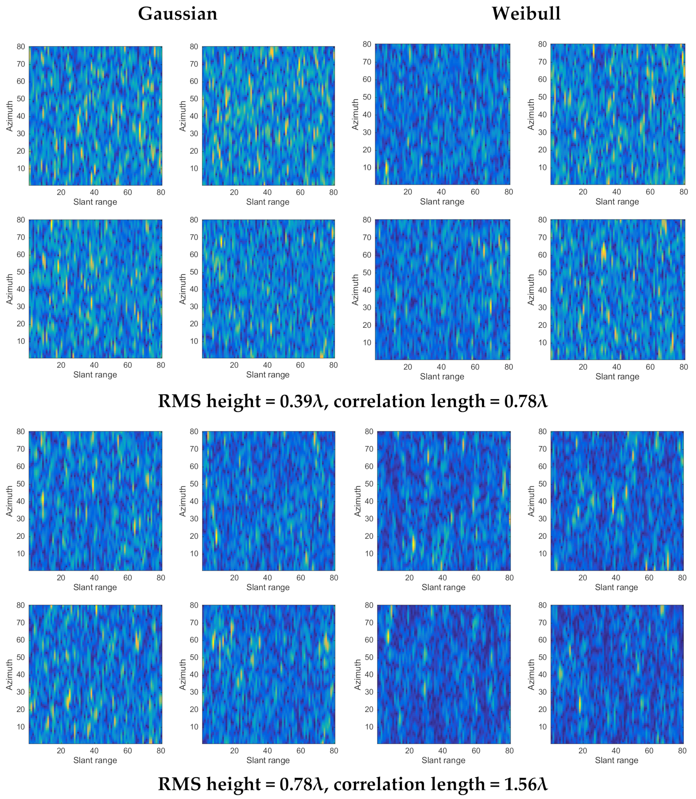
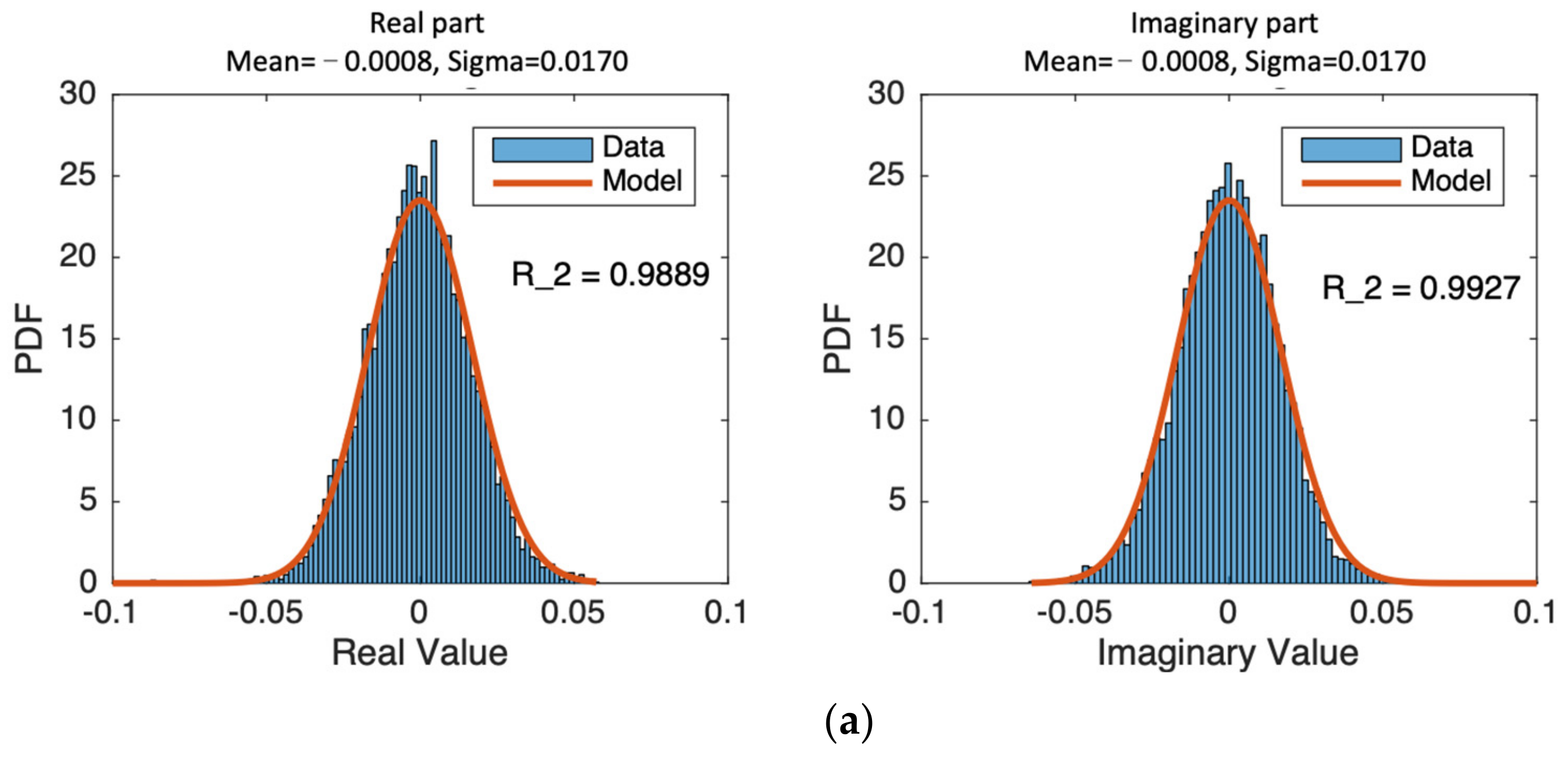
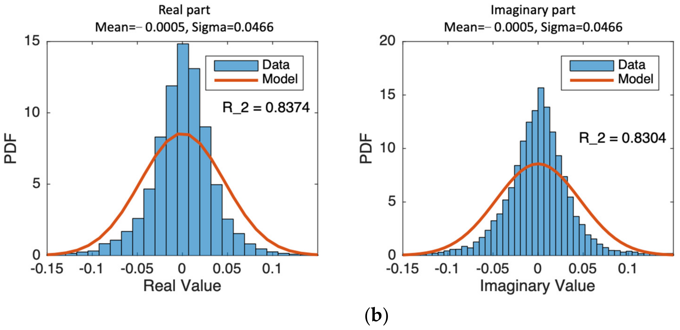
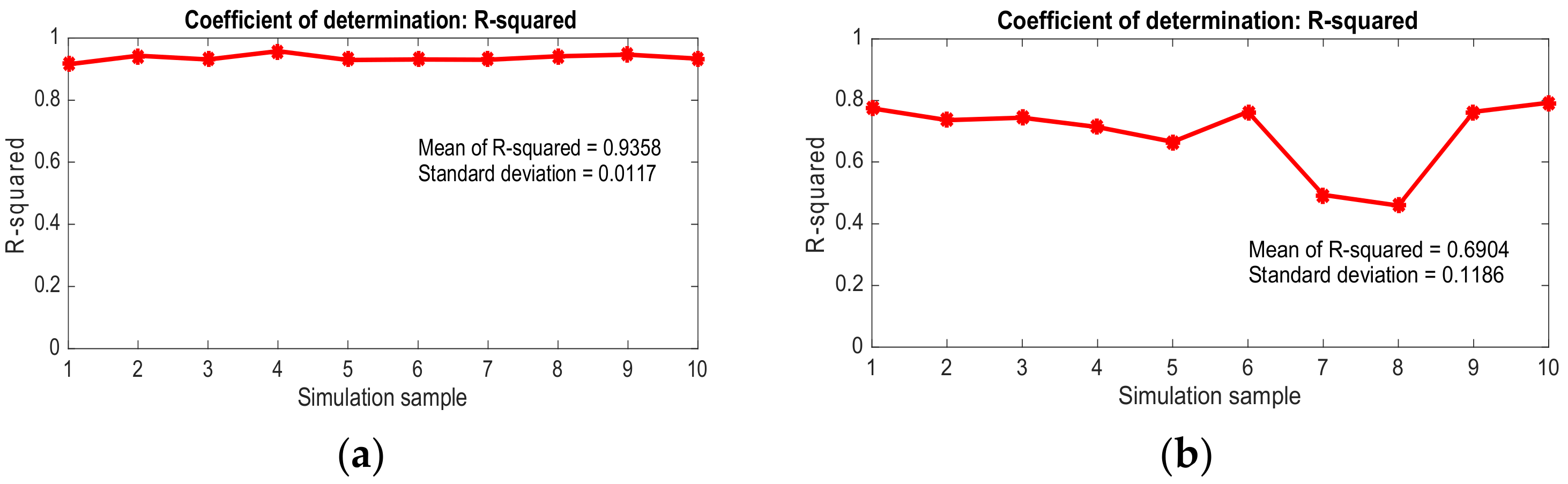
4. Statistical Properties of SAR Image of Non-Gaussian Rough Surfaces

4.1. Equivalent Number of Looks (ENL)

The Rayleigh PDF is Perhaps the most commonly used model to describe the signal statistics from many independent scatterers. Generally, multiple scatters are embedded in a single resolution, producing speckle or flicker due to random walk. As long as the resolution cell is homogeneous and ignoring the roughness effect, the speckle amplitude follows the fully developed Rayleigh speckle, regardless of the roughness parameters, including the root mean square (RMS) height and correlation length. We begin to examine the statistical properties of SAR images of non-Gaussian rough surfaces against the Rayleigh model. It is known that R2 is a statistic that will give information about the goodness of fit of a model [43]. The R2 coefficient of determination is a statistical measure of how well the regression predictions approximate the actual data points. An R2 of 1 indicates that the regression predictions perfectly fit the data in regression. For amplitude PDF to be Rayleigh, the PDFs of real and imaginary components follow the Gaussian [5,17]. Hence, we first inspected the R2 coefficients for PDFs of real and imaginary components of the SLC image against Gaussian PDF. We examined ten samples randomly selected from all 200 simulated images for every surface and radar parameter as specified in Table 2 and Table 3. Some examples are provided here and in the following sections. From Figure 6, we see that the Gaussian surface has higher R2 coefficients, of quite close to 1. On the other hand, the much lower R2 for the Weibull surface reveals its deviations from the Rayleigh model.
Next, we plotted R2 coefficients for ten samples of SLC images amplitude PDFs of Gaussian and Weibull HPD surfaces, both with exponential PSD, as shown in Figure 7. The Gaussian surface has higher and more stable R2 coefficients than the Weibull surface, indicating that the Gaussian surface tends to be more Rayleigh model. The non-Gaussian surface, or the Weibull in this case, substantially deviates from Rayleigh.
A good measure by which to inspect the speckle is the equivalent number of looks (ENL). For the N-look image of homogeneous regions, we have the Chi-Square distribution (N-1 degree of freedom) of the amplitude [5]
p N ( A ) = 2 N N σ 2 N Γ ( N ) A 2 N 1 exp ( N A 2 / σ 2 )
where σ 2 is the variance of the amplitude.
E N L N = 4 π π μ N σ N 2
where μ N is the N-look amplitude mean and σ N is the standard deviation of N-look amplitude.
Table 5 shows that the ENLs at four looks for Gaussian and Weibull HPD are different. The exponential HPD consistently gives lower ENL of the two surfaces, suggesting it produces a stronger speckle strength. There is a correlation among the pixels; the estimated number of looks is always smaller than the theoretical one. The higher the correlation indicates, the stronger speckle, hence the smaller the estimated ENL. The degree of correlation depends on the surface roughness. Generally, the rougher the surface produces stronger diffuse scattering, thereby explaining the stronger speckle. We also see the effect of N-looking in reducing the speckle variance and in increasing the accuracy of scattering coefficients or RCS estimates. However, to a different extent, such effects show for Gaussian and Weibull surfaces. When the surface slope is larger, the ENLs are moving close together. For a very smooth surface with a smaller slope, the ENLs of Gaussian and Weibull HPDs surface is very close because the coherent scattering is the dominant factor in total scattering back to the radar. Qualitative observations are also drawn for the look angles of 30° and 50°, and results are not shown here to save space.
Before proceeding, it would be of interest to discuss the simulated image speckle against those obtained from real SAR images over the sea ice, for which the surface height has non-Gaussian distribution [20]. From Figure 7, we already know from the R-squared test that the image speckle of non-Gaussian surfaces does not follow the Rayleigh distribution. Figure 8 plots the PDF of simulated image speckles for the Weibull surface with RMS height σ = 0.39 λ and correlation length = 1.56 λ at three incident angles of 30, 50, and 70 degrees. The Rayleigh model does not match the simulated data, having R2 values of only around 0.6 for three incident angles. An excellent reference of SAR image over sea ice is provided in [44]. The K distribution parameters matching the JPL airborne SAR data were also estimated. For a K distributed amplitude A , its L-look PDF is provided by [5,17]:
p ( A ) = 4 Γ ( L ) Γ ( ν ) ν L ( L + ν ) / 2 A ( L + ν 1 ) K ν L 2 A ν L 1 / 2
where K ν L ( ) is the modified Bessel function of order ν L . [44] provided the estimated ν values for first-year and multi-year ice but concluded that the ν value did not have significant effects on the PDF’s shape. After taking the several median values of ν , we also found that the PDFs only have a small difference. Figure 9 shows a comparison of PDF of speckle between simulated data and K distribution using ν = 5.96 [44] at incident angles of 30°, 50°, and 70°. The R2 values are higher than those with Rayleigh, as expected. We can see that speckle from non-Gaussian surfaces generally follows the K-distribution closely. A speckle strength is smaller at a higher incident angle, particularly at 70° incidence—a lower backscattered signal results. A more detailed analysis of the surface roughness, height distributions, and power spectral densities related to the K-distribution parameter seems necessary but is beyond the scope of this study and will instead be pursued in future studies.

4.2. Rough Surface Index (RSI)

The estimated ENLs for Gaussian and Weibull surfaces are provided in Table 5, and to some degree reveal the impact of HPD; it is still difficult to differentiate the surface’s HPD. The reason is that the ENL involves several factors, including the radar and roughness parameters. As a result, we come to define the following rough surface index (RSI):
R S I E N L = 1 3 R L 1 2 1 + 1 / E N L 1 + R L 1 , R e a l 2 + R L 1 , I m a g 2 , [ 0 , 1 ]
where R L 1 2 is the coefficient of determination for the estimated ENL; R L 1 , R e a l 2 and R L 1 , I m a g 2 are the coefficient of determination for the real and imaginary components of the complex SLC image, respectively. For a better match, the R L 1 2 , R L 1 , R e a l 2 and R L 1 , I m a g 2 are closer to 1. When the E N L   approaches 1, the real and imaginary parts of SLC data approach to a Gaussian PDF, and the amplitude follows the Rayleigh PDF, meaning that the surface tends to be more homogeneous, thereby producing uniform scatterers. For a worst case, the R L 1 2 , R L 1 , R e a l 2 and R L 1 , I m a g 2 were closer to the zero.
In the following sections, we evaluate the influence of roughness parameters (correlation length, RMS height) on image statistics using RSI measure for each set of SAR images of HPD and PSD rough surfaces at three look angles of 30, 50, and 70 degrees. To proceed, we first examine the effect of correlation length by fixing the RMS height at 0.39λ and varying the correlation lengths 0.78λ, 1.17λ, 1.56λ. Note that the ratio of correlation length to RMS height is proportional to the surface RMS slope. In this case, while increasing the correlation length with a fixed RMS height, the surface slope decreases producing a smoother rough surface. Keeping this in mind, we inspect the RSIs at different look angles, as shown in Figure 10, where the solid lines denote the Gaussian HPD surface and dash lines denote the Weibull HPD surface. In general, the RSI of the Gaussian HPD surface is higher than that of the Weibull HPD surface. The RSIs remain constant for the Gaussian HPD surfaces over three surface slopes for all three look angles. We may equivalently state that the Gaussian HPD surface tends to be more homogeneous in the context of SAR imaging. The homogeneity breaks down in the case of Weibull HPD surface, as clearly indicated by the varying RSI with the correlation length—the larger the correlation length, the higher degree of heterogeneity, again, in the context of SAR imaging, according to the image statistics. Additionally, we found that a steeper look angle produces an even lower RSI value, implying that the Gaussian distribution of both real and imaginary parts of the SLC image is no longer valid. The strong dependence of ENL on the look angle for the Weibull HPD surface is physically explained by a larger look angle, more point-like scatterers present to produce more strong-scattering pixels. We can reach a quick conclusion that the Non-Gaussian height distributed rough surface produce non-Rayleigh speckle, even more so for a smoother surface. It is unnecessary to have a very rough surface at a near-grazing angle to generate a spike-like speckle. Among the two factors, compared to the correlation length, the look angle is more dominant to drive the RSI away from unity, as indicated in Figure 10b. We also notice that the quick drop of the RSI at 70° of incidence is mainly due to very low returns. The effective scatterers responsible for the radar backscattering at such a high-looking angle (or incident angle) are drastically reduced. The angular behavior of the backscattered signal is highly nonlinear at the region of moderate to large incident angles.
Now, by fixing the correlation length while varying the RMS height from 0.39λ, 0.52λ, and 0.78λ, the surface slope increases with RMS height, resulting in a rougher surface. By observing the RSI in Figure 11a, we see that the RSI of the Gaussian HPD surface remains relatively constant over the three slopes for three look angles of 30, 50, and 70 degrees. We observe a slight deviation for the case of the roughest surface at 70 degrees of look angle. The reason behind this deviation may be attributed to the presence of more strong scatterers, for Gaussian HPD surface, at a steep look angle.
On the contrary, the RSIs are lower than those of the Gaussian HPD surface, with a more significant deviation from unity. Interestingly, the Weibull HPD surface tends to be more heterogeneous even for a smoother surface (slight slope), as revealed in Figure 11b. This trend of RSI variation over the surface slope is consistent with the results of Figure 8.
Figure 12 displays the RSIs for Gaussian and Weibull HPDs rough surface with fixed ratios of correlation length to RMS height of 0.13λ/0.26λ, 0.39λ/0.78λ, 0.78λ/1.26λ, respectively. Hence, the surface slope was found to be a constant. Accordingly, we examined the RSI dependence on the radar wavelength or frequency in this case. The results show that the RSIs between Gaussian and HPDs were close regardless of the look angle for smaller roughness or lower radar frequency. As the RMS slope increases, the RSIs start to deviate, especially at 70° of look angle. Looking at individual RSI, we see that the Gaussian HPD surface is much less sensitive to RMS height than the Weibull HPD surface. Figure 12b plots the difference of RSI as a function of roughness at three look angles to illustrate the strong dependence of RSI on roughness for Weibull HPD surface.
Table 6 below summarizes the image statistics of ENL and R2 coefficients R L 1 2   R L 1 , R e a l 2 and R L 1 , I m a g 2 of estimated ENL against Rayleigh speckle. Note that the closer the R2 to unity, the closer the speckle to the Rayleigh speckle for a single look SLC image. We see that among the R2 coefficients, the proposed R2 I is the most sensitive and effective to differentiate the image statistics between the Gaussian and Weibull HPDs surfaces. The RSI serves as a good indicator of image contrast. The RSIs are close for a small RMS height surface, implying the image contrasts of Gaussian and Weibull HPDs surface are similar. The rationale is that coherent scattering is more dominant when the surface becomes smoother. Increasing the RMS height does not impact the Gaussian HPD surface but significantly affects the Weibull surface. It should be cautioned that the statement above is provided in the context of image statistics, or more specifically, the PDF of the image intensity. It does not imply the mean strength of the intensity. Additionally, the calculated backscattering signal to SAR composes coherent and incoherent scattering components. It has been well-known that the surface HPD impacts coherent scattering. It is understood that the RMS height is critical in determining the radar returned signal. The RMS height determines the level of the backscattering coefficient, while the shape of the correlation function affects the angular behavior of the backscattering coefficient. Indeed, the incoherent scattering component is highly dependent on the surface correlation function for slightly or moderately rough surfaces. Results also confirm that as the radar frequency increases, or equivalently larger roughness, the surface HPD causes significant changes in incoherent scattering due to more multiple scattering contributions, driving the speckle farther away from the Rayleigh model. The surface HPD is the dominating factor, and and in comparison, the PSD is of a higher-order effect in the coherent scattering.

5. Conclusions

We investigated the image statistics of a non-Gaussian rough surface with a physics-based SAR Simulation approach. In simulating the SAR image, we accounted for the non-Gaussian height distribution and considered microscopic details of the roughness on comparable radar wavelength scales to include specularly, singly, and multiply scatterers. To compute the SAR-scattered fields in aperture synthesizing, we developed a numerical improved Kirchhoff approximation to estimate the surface fields. The total scattered field to SAR includes diffraction and the scattered fields due to the surface fields.
The results show that the exponential HPD gives lower ENL of the two surfaces, suggesting a stronger speckle strength it produces. When the surface slope is larger, their ENLs are found to be closer together. For a very smooth surface with a smaller slope, the ENLs of Gaussian and Weibull HPDs surface are very close because coherent scattering is the dominant factor in total backscattering.
The proposed RSI serves as a good indicator of image contrast. The RSIs are close for a small RMS height surface, implying that the Gaussian and Weibull HPDs surface image contrasts are similar, which can be explained physically because the coherent scattering is more dominant when the surface becomes smoother. Increasing the RMS height does not impact the Gaussian HPD surface but significantly affects the Weibull surface. The results also confirm that as the radar frequency increases, or the roughness increases, the surface HPD causes sufficiently significant changes in incoherent scattering due to more frequent multiple scattering contributions, driving the speckle farther away from the Rayleigh model. Looking at individual RSI, we see that the Gaussian HPD surface is much less sensitive to RMS height than the Weibull HPD surface. We demonstrated the strong dependence of RSI on roughness for non-Gaussian, Weibull HPD surface. The multi-looking effects in reducing the speckle variance and increasing the accuracy of scattering coefficients or RCS estimates show different extent for Gaussian and Weibull surfaces. The results demonstrate that to retrieve the surface parameters (both dielectric and roughness) from the estimated RCS, we expect less accuracy for the non-Gaussian surface than the Gaussian surface under the same conditions. Therefore, the results drawn from this study are helpful for conducting a system performance evaluation, parameters estimation, and target detection for SAR imaging of a rough surface. Further research could further test the first-year and multi-year sea ice surfaces. The wind-blown dunes and wind-sculpture Sastrugi surfaces are other examples to investigate.

Author Contributions

Conceptualization, K.-S.C.; methodology, K.-S.C. and C.-Y.C.; software, C.-Y.C.; validation, C.-Y.C., Y.Y. and Y.Z.; formal analysis, C.-Y.C. and K.-S.C.; investigation, K.-S.C., Y.Y. and L.W.; resources, C.-Y.C. and Y.Z.; data curation, C.-Y.C.; writing—original draft preparation, K.-S.C. and C.-Y.C.; writing—review and editing, K.-S.C. and Y.Y.; visualization, C.-Y.C., Y.Y. and L.W.; supervision, K.-S.C.; project administration, K.-S.C.; funding acquisition, K.-S.C. All authors have read and agreed to the published version of the manuscript.

Funding

This work was supported by the initiative funding of Xuchang University to C. Y. Chiang, the Guangxi Natural Science Youth Fund under Grant 2020GXNSFBA297105, National Natural Science Foundation of China under Grant 61931021, and Guangxi Natural Science Fund for Innovation Research Team under Grant 2019GXNSFGA245001.

Institutional Review Board Statement

Not applicable.

Informed Consent Statement

Not applicable.

Data Availability Statement

Not applicable.

Conflicts of Interest

The authors declare no conflict of interest.

References

  1. Guérin, C.A.; Holschneider, M.; Saillard, M. Electromagnetic scattering from multiscale rough surfaces. Waves Random Media 1997, 7, 331–349. [Google Scholar] [CrossRef]
  2. Zribi, M.; Ciarletti, V.; Taconet, O. Validation of a Rough Surface Model Based on Fractional Brownian Geometry with SIRC and ERASME Radar Data over Orgeval. Remote Sens. Environ. 2000, 73, 65–72. [Google Scholar] [CrossRef]
  3. Mattia, F.; Le Toan, L.; Davidson, M. An analytical, numerical, and experimental study of backscattering from multiscale soil surfaces. Radio Sci. 2001, 36, 119–135. [Google Scholar] [CrossRef]
  4. Zribi, M.; Baghdadi, N.; Holah, N.; Fafin, O. New methodology for soil surface moisture estimation and its application to ENVISAT-ASAR multi-incidence data inversion. Remote Sens. Environ. 2005, 96, 485–496. [Google Scholar] [CrossRef]
  5. Lee, J.S.; Pottier, E. Polarimetric Radar Imaging: From Basics to Applications; CRC Press: Boca Raton, FL, USA, 2009. [Google Scholar]
  6. Kazuo, O.; Shahram, T.; Ronald, E.B. Dependence of speckle statistics on backscatter cross-section fluctuations in synthetic aperture radar images of rough surfaces. IEEE Trans. Geosci. Remote Sens. 1987, GE-25, 623–628. [Google Scholar]
  7. Yueh, S.H.; Kong, J.A.; Jao, J.K.; Shin, R.T.; Novak, L.M. K-distribution and polarimetric terrain radar clutter. J. Electromagn. Waves Appl. 1989, 3, 747–768. [Google Scholar] [CrossRef]
  8. Sarabandi, K.; Oh, Y. Effect of Antenna Footprint on the Statistics of Radar Backscattering from Random Surfaces. In Proceedings of the 1995 International Geoscience and Remote Sensing Symposium, IGARSS ′95. Quantitative Remote Sensing for Science and Applications, Firenze, Italy, 10–14 July 1995; pp. 927–929. [Google Scholar]
  9. Nesti, G.; Fortuny, J.; Sieber, A.J. Comparison of backscattered signal statistics as derived from indoor scatterometric and SAR experiments. IEEE Trans. Geosci. Remote Sens. 1996, 34, 1074–1083. [Google Scholar] [CrossRef]
  10. Franceschetti, G.; Migliaccio, M.; Riccio, D. An electromagnetic fractal-based model for the study of fading. Radio Sci. 1996, 31, 1749–1759. [Google Scholar] [CrossRef]
  11. Martino, G.D.; Iodice, A.; Riccio, D.; Ruello, G. Physical-Based Models of Speckle for High Resolution SAR Images. In Proceedings of the IEEE International Geoscience & Remote Sensing Symposium, IGARSS 2010, Honolulu, HI, USA, 25–30 July 2010; pp. 2980–2983. [Google Scholar]
  12. Martino, G.D.; Iodice, A.; Riccio, D.; Ruello, G. A physical approach for SAR speckle simulation: First results. Eur. J. Remote Sens. 2013, 46, 823–836. [Google Scholar] [CrossRef] [Green Version]
  13. Chen, K.S.; Tsang, L.; Chen, K.L.; Liao, T.H.; Lee, J.S. Polarimetric simulations of SAR at L-Band over bare soil using scattering matrices of random rough surfaces from numerical three-dimensional solutions of Maxwell equations. IEEE Trans. Geosci. Remote Sens. 2014, 52, 7048–7058. [Google Scholar] [CrossRef]
  14. Martino, G.D.; Iodice, G.; Riccio, D.; Ruello, G. Equivalent number of scatterers for SAR speckle modeling. IEEE Trans. Geosci. Remote Sens. 2014, 52, 2555–2564. [Google Scholar] [CrossRef]
  15. Jin, M.; Chen, K.S.; Xie, D.F. On the very high-resolution radar image statistics of the exponentially correlated rough surface: Experimental and numerical studies. Remote Sens. 2018, 10, 1369. [Google Scholar] [CrossRef] [Green Version]
  16. Migliaccio, M.; Huang, L.Q.; Buono, A. SAR speckle dependence on ocean surface wind field. IEEE Trans. Geosci. Remote Sens. 2019, 57, 5447–5455. [Google Scholar] [CrossRef]
  17. Cristea, A.; Doulgeris, A.P.; Eltoft, T. A Noncentral and Non-Gaussian Probability Model for SAR Data. In Proceedings of the Scandinavian Conference on Image Analysis, Tromsø, Norway, 12–14 June 2017. [Google Scholar] [CrossRef] [Green Version]
  18. Stark, H.; Woods, J.W. Probability, Random Processes and Estimation Theory for Engineers, 4th ed.; Prentice Hall: Englewood Cliffs, NJ, USA, 2011. [Google Scholar]
  19. Huang, N.E.; Long, S.R.; Tung, C.-C.; Yuan, Y.; Bliven, L.F. A non-Gaussian statistical model for surface elevation of nonlinear random wave fields. J. Geophys. Res. 1983, 88, 7597. [Google Scholar] [CrossRef]
  20. Brown, G.S. A theory for near-normal incidence microwave scattering from first-year sea ice. Radio Sci. 1982, 17, 233–243. [Google Scholar] [CrossRef]
  21. Beckmann, P. Scattering by non-Gaussian surfaces. IEEE Trans. Antenna Propag. 1973, AP-21, 169–175. [Google Scholar] [CrossRef]
  22. Brown, G.S. Scattering from a class of randomly rough surfaces. Radio Sci. 1982, 17, 1274–1280. [Google Scholar] [CrossRef]
  23. Eom, H.J.; Fung, A.K. A comparison between backscattering coefficients using Gaussian and non-Gaussian surface statistics. IEEE Trans. Antennas Propag. 1983, AP-31, 635–638. [Google Scholar] [CrossRef]
  24. Wu, S.C.; Chen, M.F.; Fung, A.K. Scattering from non-gaussian randomly rough surfaces-cylindrical case. IEEE Trans. Geosci. Remote Sens. 1988, 26, 790–798. [Google Scholar] [CrossRef]
  25. Pérez-Ràfols, F.; Almqvist, A. Generating randomly rough surfaces with given height probability distribution and power spectrum. Tribol. Int. 2019, 131, 591–604. [Google Scholar] [CrossRef]
  26. Jiang, R.; Chen, K.S.; Li, Z.L.; Du, G.Y.; Tian, W.J. Entropy measure of generating random rough surface for numerical simulation of wave scattering. IEEE Trans. Geosci. Remote Sens. 2020, 59, 3623–3641. [Google Scholar] [CrossRef]
  27. Hodaei, M.; Farhang, K. Effect of rough surface asymmetry on contact energy loss in hip implants. J. Mech. Med. Biol. 2016, 17, 1750023. [Google Scholar] [CrossRef]
  28. Chen, K.S. Radar Scattering and Imaging of Rough Surface: Modeling and Applications with MATLAB®; CRC Press: Boca Raton, FL, USA, 2020. [Google Scholar]
  29. Church, E.L.; Takacs, P.Z.; Stover J, C. Light Scattering from Non-Gaussian Surfaces. In Proceedings of the SPIE-The International Society for Optical Engineering, San Diego, CA, USA, 13–14 July 1995; Volume 2541, pp. 91–107. [Google Scholar]
  30. Bendat, J.S.; Piersol, A.G. Random Data: Analysis and Measurement Procedures, 4th ed.; John Wiley & Sons, Inc.: Hoboken, NJ, USA, 2010. [Google Scholar]
  31. Chen, K.S. Principles of Synthetic Aperture Radar Imaging: A System Simulation Approach; CRC Press: Boca Raton, FL, USA, 2016. [Google Scholar]
  32. Blackledge, J.M. Quantitative Coherent Imaging: Theory, Methods and Some Applications; Academic Press: New York, NY, USA, 2012. [Google Scholar]
  33. Frey, P.J.; George, P.L. Mesh Generation: Application to Finite Elements, 2nd ed.; ISTE Ltd. and John Wiley & Sons: Hoboken, NJ, USA, 2008. [Google Scholar]
  34. Tsang, L.; Ding, K.H.; Huang, S.H.; Xu, X. Electromagnetic computation in scattering of electromagnetic waves by random rough surface and dense media in microwave remote sensing of land surfaces. Proc. IEEE 2013, 101, 255–279. [Google Scholar] [CrossRef]
  35. Boardman, T. Getting Started in 3D with 3ds Max; Focal Press: Burlington, MA, USA, 2013. [Google Scholar]
  36. Jing, J.M. Theory and Computation of Electromagnetic Fields, 2nd ed.; Wiley-IEEE Press: New York, NY, USA, 2015. [Google Scholar]
  37. Graglia, R.D.; Peterson, A.F. Higher-Order Techniques in Computational Electromagnetics; SciTech Publishing: Raleigh, NC, USA, 2016. [Google Scholar]
  38. Fung, A.K. Microwave Scattering and Emission Models and Their Applications; Artech House: Norwood, MA, USA, 1994. [Google Scholar]
  39. Fung, A.K.; Li, Z.; Chen, K.S. Backscattering from a randomly rough dielectric surface. IEEE Trans. Geosci. Remote Sens. 1992, 30, 356–369. [Google Scholar] [CrossRef]
  40. De Adana, F.S.; Diego, I.G.; Blanco, O.G.; Lozano, P.; Catedra, M.F. Method based on physical optics for the computation of the radar cross section including diffraction and double effects of metallic and absorbing bodies modeled with parametric surfaces. IEEE Trans. Antennas Propagat. 2004, 52, 3295–3303. [Google Scholar] [CrossRef]
  41. Knott, E.F.; Senior, T.B.A. Comparison of three high-frequency diffraction techniques. Proc. IEEE 1974, 62, 1468–1474. [Google Scholar] [CrossRef]
  42. Cumming, I.; Wong, F. Digital Signal Processing of Synthetic Aperture Radar Data: Algorithms and Implementation; Artech House: Norwood, MA, USA, 2004. [Google Scholar]
  43. Chicco, D.; Warrens, M.J.; Jurman, G. The coefficient of determination R-squared is more informative than SMAPE, MAE, MAPE, MSE and RMSE in regression analysis evaluation. J. Comput. Sci. 2021, 7, e623. [Google Scholar] [CrossRef]
  44. Joughin, I.R.; Percival, D.B.; Winebrenner, D.P. Maximum likelihood estimation of K distribution parameters for SAR data. IEEE Trans. Geosci. Remote Sens. 1993, 31, 989–999. [Google Scholar] [CrossRef]
Figure 1. Samples of generated rough surfaces with HPD: (a) Gaussian, (b) Weibull (shape parameter: 1.8). The left panel is sample surface heights, the right panel shows HPDs with red-line denoting the model, and the histogram is the HPD simulated data).
Remotesensing 14 00311 g001
Figure 2. Geometry of strip-map mode SAR imaging of a rough surface.
Remotesensing 14 00311 g002
Figure 3. Schematic illustration of the scattering paths due to the incident field upon patches of a scattering body, shown are (a) near-field scattering over the scattering body; (b) a local coordinate system formed by ( k ^ i , n ^ , t ^ ) . Antenna pattern effect is not shown.
Remotesensing 14 00311 g003
Figure 4. Focused SAR amplitude image. A full SAR map (left) and region of interest image (right).
Remotesensing 14 00311 g004
Figure 5. Sample SLC images of Gaussian HPD surface (left panel) and Weibull HPD surface (right panel). Two roughness (RMS height and correlation length) are considered.
Remotesensing 14 00311 g005
Figure 6. PDFs of Real and imagery parts of SLC images, (a): Gaussian HPD surface; (b) Weibull HPD surface. The surface RMS height is 0.39λ, correlation length is 1.56λ, with look angle of 70°.
Remotesensing 14 00311 g006aRemotesensing 14 00311 g006b
Figure 7. R2 coefficients of amplitude PDF of SLC images against the Rayleigh model: (a) HPD: Gaussian; (b) HPD: Weibull. The PSD for both surfaces is exponential.
Remotesensing 14 00311 g007
Figure 8. Comparison of PDF of speckle between simulated data and Rayleigh distribution at incident angles of 30° (a), 50° (b), and 70° (c). The R2 values for each case are shown. Surface parameters: Weibull HPD, exponential PSD with RMS height σ = 0.39 λ and correlation length = 1.56 λ .
Remotesensing 14 00311 g008
Figure 9. Comparison of PDF of speckle between simulated data and K distribution at incident angles of 30° (a), 50° (b), and 70° (c). The R2 values for each case are shown. Surface parameters: Weibull HPD, exponential PSD with RMS height σ = 0.39 λ and correlation length = 1.56 λ .
Remotesensing 14 00311 g009
Figure 10. Comparison of RSI between Gaussian and Weibull HPDs surface as a function of correlation length, at three look angles of 30, 50, and 70 degrees; (a) RSI, (b) Difference of RSIs.
Remotesensing 14 00311 g010
Figure 11. Comparison of RSI between Gaussian and Weibull HPDs surface as a function of RMS height, at three look angles of 30, 50, and 70 degrees; (a) RSI, (b) Difference of RSIs.
Remotesensing 14 00311 g011
Figure 12. Rough surface index (RSI) for three roughness scales of 0.13λ/0.26λ, 0.39λ/0.78λ, 0.78λ/1.26λ. (a) RSI, (b) Difference of RSIs.
Remotesensing 14 00311 g012
Table 1. Statistics of generated roughness surface.
RMS Height [λ]Correlation Length [λ]Simulated
RMS Height [λ]
(Gaussian HPD/Weibull HPD)
Simulated
Correlation Length at x-Direction [λ]
(Gaussian PSD/Exponential PSD)
Simulated
Correlation Length at y-Direction [λ]
(Gaussian PSD/Exponential PSD)
0.130.260.1300/0.13000.2656/0.26500.2655/0.2649
0.390.780.3900/0.39010.7855/0.78140.7852/0.7809
0.781.560.7799/0.78011.5535/1.54171.5527/1.5384
0.1950.780.1950/0.19500.7855/0.78140.7852/0.7809
0.391.560.3900/0.39011.5535/1.54171.5527/1.5384
0.521.560.5199/0.52011.5535/1.54171.5527/1.5384
Table 2. Surface parameters.
ParameterValue
Surface size (Lx, Ly)120 × 120 [λ]
Surface sampling number (Nx, Ny)2048 × 2048 [samples]
Correlation length ( )0.26, 0.78, 1.56 [λ]
Root mean square height ( s )0.13, 0.195, 0.39, 0.78 [λ]
Dielectric constant20-j4.0
Table 3. The SAR simulation parameters.
ParameterValue
Center frequency1.27 GHz
Sampling rate591 MHz
Chirp bandwidth591 MHz
PRF213.4 Hz
Duty cycle6.8%
Antenna size0.5 m × 5.2 m
Reference ellipsoidWGS84
Look angle72/50/30 degrees
PolarizationHH
Range dimension350 samples
Azimuth dimension1100 samples
Table 4. Doppler coefficient & Resolution & Sampling.
ParameterValue
Azimuth effective antenna size0.4929 m
Doppler rate15.94 Hz/s
Exposure time12.2035 s
Doppler bandwidth194.5791 Hz
Range resolution0.2536 m
Azimuth resolution0.2463 m
Range spacing0.2536 m
Azimuth spacing0.2536 m
Table 5. The ENL of 1~4 looks estimated for Gaussian and Weibull surfaces at various roughness parameters (RMS height and correlation length). The SAR look angle is 72°.
Roughness
(λ)
ENL
Gaussian HPD
ENL
Weibull HPD
Look = 1Look = 2Look = 3Look = 4Look = 1Look = 2Look = 3Look = 4
σ = 0.13
l = 0.26
0.92541.76562.53743.26560.97111.69082.26012.8752
σ = 0.39
l = 0.78
0.97161.68782.32562.91200.93411.29691.55341.7316
σ = 0.78
l = 1.56
0.95871.71942.48843.09140.92201.40111.78622.2119
σ = 0.195
l = 0.78
0.98651.54522.08542.52730.95111.17811.30041.3809
σ = 0.39
l = 1.56
0.98851.69482.36052.93150.92201.31011.50761.7723
Table 6. Estimated ENL and R2 coefficients under various roughness scale for Gaussian and Weibull HPDs surfaces.
Roughness
(λ)
~Slope
(s/l)
HPDENLR2 (Avg.)R2L1, realR2L1, imagRSI
Look = 1Look = 1Look = 1Look = 1Look = 1
σ = 0.13
l = 0.26
1:2Gaussian1.10110.97790.98790.98550.9692
Weibull0.99260.93590.98840.98660.9690
σ = 0.39
l = 0.78
1:2Gaussian1.02350.97780.98830.98500.9798
Weibull1.12200.94670.90620.90290.8655
σ = 0.78
l = 1.56
1:2Gaussian0.79540.97780.98160.97760.9435
Weibull0.46880.80520.67570.68680.6337
σ = 0.195
l = 0.78
1:4Gaussian1.09360.98430.98990.98650.9733
Weibull1.01740.96290.97800.97320.9690
σ = 0.39
l = 1.56
1:4Gaussian0.98530.98430.98750.98910.9843
Weibull0.81590.95670.90760.89230.8856
Publisher’s Note: MDPI stays neutral with regard to jurisdictional claims in published maps and institutional affiliations.

