Technical Note

Climatology and Long-Term Trends in the Stratospheric Temperature and Wind Using ERA5

1
Institute of Atmospheric Physics CAS, 14100 Prague, Czech Republic
2
Department of Atmosperic Physics, Faculty of Mathematics and Physics, Charles University, 18000 Prague, Czech Republic
*
Author to whom correspondence should be addressed.
Remote Sens. 2021, 13(23), 4923; https://doi.org/10.3390/rs13234923
Submission received: 11 October 2021 / Revised: 27 November 2021 / Accepted: 30 November 2021 / Published: 3 December 2021
(This article belongs to the Special Issue GNSS Atmospheric Modelling)

Abstract

:
This study analyses long-term trends in temperature and wind climatology based on ERA5 data. We study climatology and trends separately for every decade from 1980 to 2020 and their changes during this period. This study is focused on the pressure levels between 100–1 hPa, which essentially covers the whole stratosphere. We also analyze the impact of the sudden stratospheric warmings (SSW), North Atlantic Oscillation (NAO), El Nino Southern Oscillation (ENSO) and Quasi-biennial oscillation (QBO). This helps us to find details of climatology and trend behavior in the stratosphere in connection to these phenomena. ERA5 is one of the newest reanalysis, which is widely used for the middle atmosphere. We identify the largest differences which occur between 1990–2000 and 2000–2010 in both temperature climatology and trends. We suggest that these differences could relate to the different occurrence frequency of SSWs in 1990–2000 versus 2000–2010.

1. Introduction

The study of processes in the middle atmosphere is essential for understanding the dynamics of the whole atmosphere. The most monitored parameter for describing conditions and changes in the middle atmosphere is undoubtedly air temperature. Temperature is connected not only with dynamics, but also with chemical processes. That is why we need to know the detailed behavior of this parameter during the last 40 years. Temperature changes in the middle atmosphere have been detected in recent decades. Between 1979 and 2018, satellite data showed a global stratosphere cooling by approximately 1–3 K [1]. However, this cooling is not linear and was more pronounced in the first half of this period, particularly in the lower stratosphere. Temperature trends in the lower stratosphere are also affected substantially by the ozone depletion and its potential recovery. They may be affected by many phenomena such as NAO (North Atlantic Oscillation), SSW (sudden stratospheric warming) or the presence of aerosols from volcanic activity. For example, the eruption of the Pinatubo volcano in 1991 caused temporary warming of this layer for two years [2]. The negative temperature trends around −0.2 to −0.3 degrees per decade in the lower stratosphere are confirmed by [3] based on the MERRA2 and ERA5 reanalysis data for 1980–2019. The temperature changes in the higher parts of the middle atmosphere are discussed in more detail in many studies, e.g., [4,5], confirming the cooling of the stratosphere and mesosphere. Chemistry–climate models can also be used to analyze temperature trends, with the possibility of simulations of different radiative forcing and ozone-depleting substances emissions, e.g., [6,7].
The stratospheric horizontal wind is another key factor which is worthy of research. The stratospheric wind, zonal and generally much weaker meridional, is characterized by high variability. The problem with analyzing stratospheric wind is the lack of direct observations in the middle and higher stratosphere. Long-term oscillations analysis based on ground-based microwave Doppler Wind Radiometer (WIRA) measurements between 5 hPa and 0.02 hPa shows a strong seasonality with higher amplitudes during the winter [8]. Naturally induced variability, especially zonal wind response to the 11-year solar cycle, has been analyzed by [9]. The influence of geomagnetic activity on the zonal wind in the Northern Hemisphere (NH), especially in relation to the polar vortex, is assessed by [10]. Stratospheric wind contributes significantly to the distribution of ozone as a part of the meridional Brewer–Dobson circulation [11]. The winter meridional wind at northern midlatitudes has been investigated by [12]. As ozone is the main source of heat through the absorption of solar radiation, its distribution has a major impact on temperature trends in the stratosphere. Regional changes in the amount of ozone in the stratosphere between 2001 and 2018 are described, e.g., by [13]. Seasonal ozone depletion in the Antarctic stratosphere is closely linked to the polar vortex, e.g., [14].
Disrupting the polar vortex, especially in the Northern Hemisphere, SSW fundamentally changes temperature and wind conditions in the relevant areas. Major SSWs are observed typically five or six times per decade [15]. The effect of SSW on zonal wind and temperature has been described, for example, by [16,17].
An important phenomenon affecting the equatorial zonal wind in the stratosphere is the quasi-biennial oscillation (QBO). QBO has an irregular mean period of about 28 months [18]. Wind amplitude during QBO reaches a peak of around 30 m/s at 20 hPa at the equator, based on the MERRA2 dataset [19]. Changes in QBO in CMIP6 climate projections are discussed by [20]. As the QBO index is usually used data sourced from the Singapore wind observations, when we want to use them as a global QBO index for climatological or trend studies, this limitation has to be taken into account.
Another feature of weather and climate variability with an impact on temperature and zonal wind in the stratosphere over the Northern Hemisphere could be the North Atlantic Oscillation (NAO). This parameter is very important for the NH dynamics, especially in the troposphere. Its impact on the stratosphere should be visible mainly in the lower stratosphere.
As previously mentioned, mainly direct observations (satellite or ground based) or chemistry-climate models (WACCM, etc.) have been used for analyzing temperature and wind climatology and trends. These datasets, especially the observations, are not always consistent in time or space and some gaps can occur. That is why reanalysis are used for these studies. We will use ERA5 reanalysis, which is one of the newest broadly used reanalysis in atmospheric studies.
This study shows us the climatology and trends in the stratosphere during the last four decades. It will also show a brief comparison between the GPS RO observations, MERRA-2 reanalysis and ERA5 reanalysis. Analyzing all grid points instead of zonal averaging will provide an overview of which regions should be analyzed in more detail.

2. Materials and Methods

We use ECMWF (European Center for Medium-Range Weather Forecasts) reanalysis ERA5. Its detailed description can be found in ERA5 data documentation or in [21], available online: https://software.ecmwf.int/wiki/display/CKB/ERA5+data+documentation (accessed on 18 July 2021). Data have been downloaded from: https://cds.climate.copernicus.eu/cdsapp#!/dataset/reanalysis-era5-pressure-levels-monthly-means?tab=form (accessed on 2 August 2021). ERA5 is available from 1980 until the present on an hourly basis, but in the present study we use monthly mean values for each parameter (temperature, zonal wind). ERA-5 has the resolution 0.75 × 0.75.
Modern Era Retrospective-Analysis for Research and Applications (MERRA2, details in [22]), was downloaded from https://disc.gsfc.nasa.gov/daac-bin/FTPSubset2.pl (accessed on 18 April 2019). MERRA2 has the resolution of 0.5 degree in latitude and 2/3 in longitude and is available from 1980 until the present.
As observations, we used data from the global positioning system (GPS). The radio occultation (GPS RO) technique is an active limb-sounding observation of the Earth’s atmosphere. The neutral atmospheric profiles retrieved from COSMIC-1 radio occultation (RO) data have been demonstrated to be very useful for studying atmospheric processes [15,23]. GPS (GNSS) RO data are highly accurate; they were used among others to calibrate AMSU instruments onboard satellites [23]. That is why they can be useful for analyzing atmospheric dynamics, including trend analysis in the troposphere and stratosphere. The vertical resolution of the geometrical optics (GO) method [24] in the stratosphere is about 1.5 km due to Fresnel radius limitations, but the full spectrum inversion (FSI) [25] can provide superior resolutions. The archived GPS RO data have been calculated by applying FSI to COSMIC GPS RO profiles at altitudes from ground level up to 30 km. We used the COSMIC GPS RO profiles available at the RISH Kyoto home webpage http://database.rish.kyoto-u.ac.jp/arch/iugonet/GPS/index.html#COSMIC%20FSI%20Data (accessed on 18 May 2020).
We analyze temperature and zonal wind from 1980 to 2020 divided into four sub-periods (decades). By comparing results between these decades, we can identify changes between different decades and look for possible reasons for these changes. We computed winter (DJF for the NH and JJA for the SH) climatology and trend for each grid point for 40–90°N/S at several pressure levels (1, 5, 10, 30 and 100 hPa). These levels represent different parts of the stratosphere from the stratopause on the top to the tropopause in the bottom. The winter season was chosen because dynamics during summer season are not so pronounced. Trend is computed as a linear ordinary least squares fit. The uncertainty estimates of the trends are set at a 95% confidence level. We do not use zonal averages because information about the structure of the results can be lost; therefore, individual grid points are analyzed. We use a time series of several stratospheric phenomena such as QBO, NAO, ENSO or SSW to identify the possible influence of each parameter on the climatology or trend.

3. Results

We analyze temperature and wind climatology and trends using ERA5 reanalysis during 1980–2020. Temperature climatology and trend from ERA5 reanalysis is compared with MERRA2 for the period 1980–2020. Figure 1 shows that the main features for climatology and trend analysis at 1, 10, 50 and 100 hPa are very similar in terms of location or amplitude. If we look at the trend comparison, the biggest differences can be found for 1 hPa, but for the lower pressure levels the main features are similar even when the amplitude is different. We also analyze a comparison of two reanalyses with GPS RO for the limited period 2010–2020, see [26]. From the comparison of two main reanalyses for a longer period and with GPS RO for a shorter period, we can say that at least down from 10 hPa ERA5 is suitable for our analysis. We can also find detailed information about comparison GPS RO and other reanalysis in [27], especially in chapter 3.7.2. Unfortunately, ERA5 is not included in [27].
Figure 2 and Figure 3 show temperature climatology and their differences for five pressure levels and four decades. At 1 and 5 hPa we can identify a two-cell structure for all decades. Lower temperature is observed over Canada and the Northern Pacific and higher temperature over the Northern Atlantic and Euroasian continent. At 30 and 100 hPa, this structure is not so pronounced but is still visible. In the Southern Hemisphere, the temperature field is consistent because winter conditions in the SH are more stable than in the NH. We can identify a negative difference between the decades of 2000–2010 and 1990–2000 (−4 K difference) on the NH at 1 and 5 hPa. On the other hand, there is a positive difference (4 K) between the same decades at lower pressure levels (100 and 30 hPa). This result shows that the temperature behavior is different in the lower and upper stratosphere. Furthermore, we identify strong positive differences between the decades of 2000–2010 and 1990–2000 on the SH at 1 hPa, but negative one at 5 hPa. This change reaches up to almost 8 K. At lower pressure levels the differences are much smaller (around 1 K).
Figure 4 and Figure 5 analyze temperature trends and their differences between decades. There is a negative trend cell over the Northern Atlantic at 1 and 5 hPa in the first three decades but in lower levels (30 and 100 hPa) this trend is smaller. In the 2000–2010 decade in particular we can observe a positive trend on the NH. Trends on the SH oscillate around 0 K/decade. Only at 1 hPa the trend is positive in the 1980–1990 and 2000–2010 decades. If we focus on the differences between decades, we identify cell structure on the NH between the decades of 1990–2000 and 1980–1990. At 1 hPa, a negative change is located over the Euroasian continent and a positive change is located over the North Atlantic at 30 and 100 hPa. The location of cells can be seen on the opposite sides (negative over the Atlantic and positive over Asia). The next feature which should be mentioned is the difference between the decades of 2000–2010 and 1990–2000. At 1 hPa on the SH the difference is positive but at lower heights the difference is negative. It is probably related to the same change in temperature climatology. Furthermore, we can identify a strong negative difference between the decades of 2010–2020 and 2000–2010 at lower levels, while at higher levels (5 hPa) a positive difference occurs.
Now, zonal wind will be analyzed, which is another very important parameter in the stratosphere. Figure 6 and Figure 7 show zonal wind averages and their difference between decades. The main result is that we can see almost no structure on the SH for all pressure levels and decades. This confirms that general circulation on the SH is stable without any large disturbances. On the NH, we identify westerly wind cell over the Northern Atlantic, especially at higher pressure levels (1 and 5 hPa). If we focus on the difference, a complex structure occurs between 1990–2000 and 1980–1990 at almost all pressure levels. The same structure can be seen between 2010–2020 and 2000–2010. Furthermore, we can see a negative difference between 2000–2010 and 1990–2000 at 5, 10 and 30 hPa. This feature is supported by negative change between 2000–2010 and 1980–1990. This can indicate that we should focus on the 2000–2010 decade.
Figure 8 and Figure 9 show zonal wind trends and their changes between decades. In the first two decades we can see cell structure on the NH at higher levels (1–10 hPa) and almost no structure on the SH. On the other hand, especially in 2010–2020, there are positive trend structures on the SH. In 2000–2010 there is a strong negative trend on the NH at 5, 10 and 30 hPa. The differences between the decades of 1990–2000 and 1980–1990 are negative over the America and North Atlantic sector and positive over Asia at 1, 5 and 10 hPa on the NH, but are mostly negative at 30 and 100 hPa. The opposite structure can be seen between 2000–2010 and 1990–2000. The positive change is visible on the NH between the decades of 2010–2020 and 2000–2010.

4. Discussion

Comparisons of observations or model simulations with results from reanalysis datasets are an important aspect of evaluating and understanding stratospheric dynamics and providing confidence for future predictions. The biggest problem with the comparison of our results with other studies is that trends or climatology, especially for temperature, are as a rule presented as global or zonal means, whereas we present results for individual grid points. If we look at our results, e.g., Figure 2 or Figure 4, we can identify cell structures. This is due to the presence of a stationary planetary wave with zonal wavenumber 1 [28]. Such information is lost during zonal averaging. On the other hand, if we consider [27], the main features for temperature and wind climatology agree in terms of their amplitude in specific regions (polar region or middle latitudes).
Temperature and zonal wind climatology (Figure 2 and Figure 6) are in general agreement with other studies [9,27,29,30,31]. We can identify cell structure on the NH at the higher altitudes and this structure is much weaker in the lower stratosphere. The structure in climatology on the SH is much less pronounced because the dynamics on the SH are stable and almost without major SSWs.
Figure 4 shows temperature trends over the last four decades. Even if we cannot compare results directly, we can see agreement between studies which confirm stratospheric cooling and tropospheric warming [1 or 6] and our results where trends are negative at the higher levels and positive at about 100 hPa.
The analysis of changes in climatology and trends during the last four decades is also very important for understanding the influence of different phenomena in the stratosphere. Figure 10 shows several important phenomena, which could significantly influence the stratospheric dynamics and vice versa. Variations of NAO and probably ENSO are much lower during the 2000–2010 decade. This coincides with our results where the zonal wind climatology differences between the decade of 2000–2010 are much larger than those among other decades. The QBO influence is probably not pronounced in our results. A detailed description of QBO can be found in [32]. The only disruption of QBO was found in 2016 and the possible reason for this is discussed in [33]. The behavior of solar radio flux F107 is similar for the first three decades but solar activity is clearly weaker during 2010–2020. F107 was recently very carefully analyzed by Clette [34], who found a sudden upward jump of F10.7 between 1980 and 1981; this has practically no impact on our study. The influence of F10.7 does not seem to be pronounced in our results.
Now we will focus on the SSW. The WMO major warming definition is used [35]. This phenomenon has been derived from MERRA2 reanalysis. Because the occurrence of SSW is not regular, we use them for climatology comparison only. This phenomenon can influence climatology and trends much more than other phenomena because an increase in temperature, particularly during major SSWs, can reach up to 60 K and together with the zonal wind reversal can last for several weeks. Examples of the behavior of temperature and zonal wind during major SSWs in 2009 and 2002 can be found in [36]. We can see that temperature in 2009 increased more than 60 K and this condition remained for almost 5 weeks. The same situation was observed for many major SSWs. It is probable that this increase will affect temperature climatology in winter significantly. Figure 11 shows that during the 1990–2000 decade, only two major SSWs occurred, while during the 2000–2010 decade there were many more major SSWs. This discrepancy is probably responsible for large differences between the decades of 1990–2000 and 2000–2010 for temperature and zonal wind climatology and trends. These results are supported by the fact that the occurrence of major SSWs in 2010–2020 decreases. In the future, we would like to compare the above results on the role of SSW with results derived from other reanalysis and with observations or climate model data to appear in the near future.

5. Conclusions

The main conclusions of this study, which was performed for winters of 1980–2020 for individual grid values in the stratosphere between latitudes 40° and 90°, are as follows:
(1)
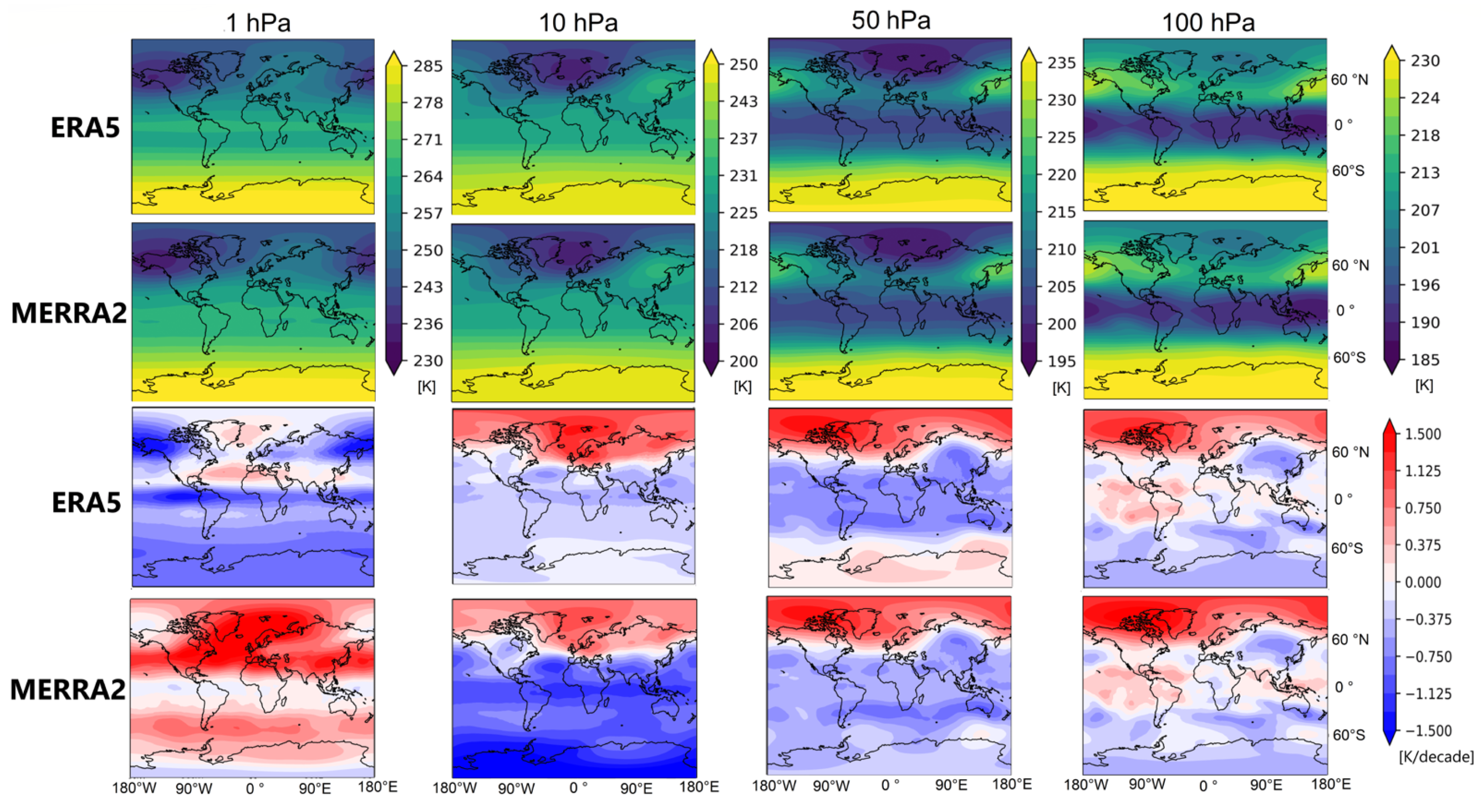
A two-cell structure occurs in the Northern Hemisphere for temperature.
(2)
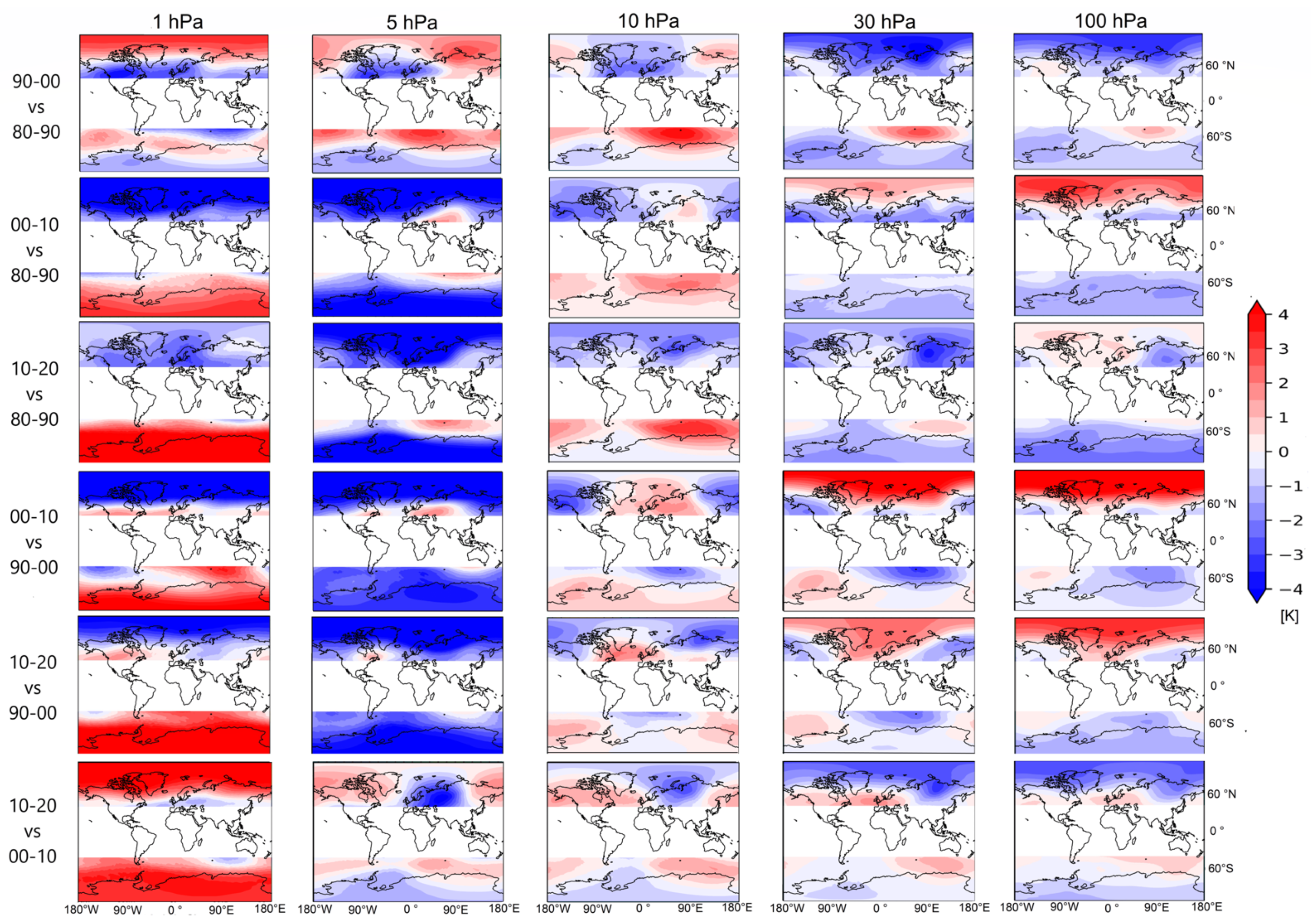
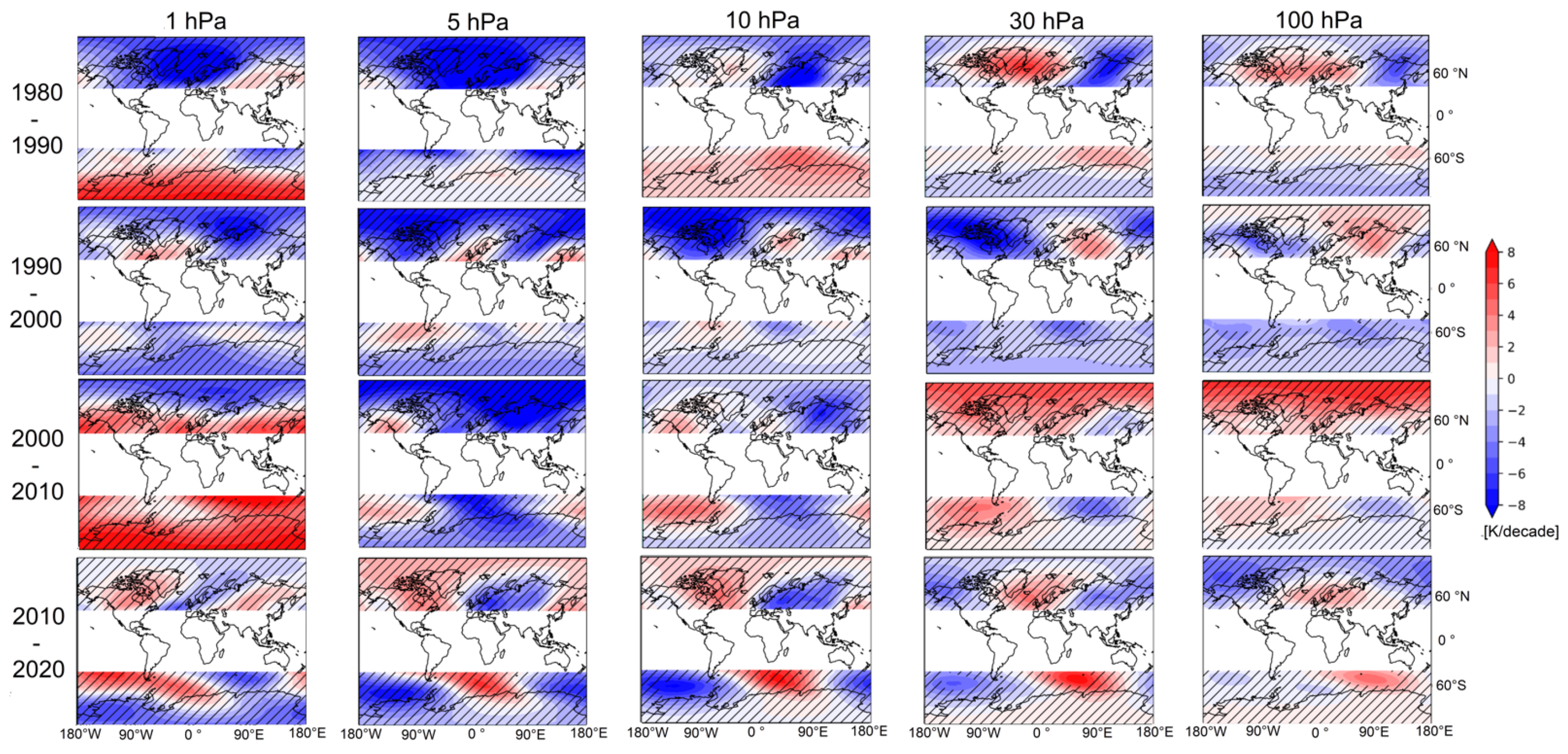
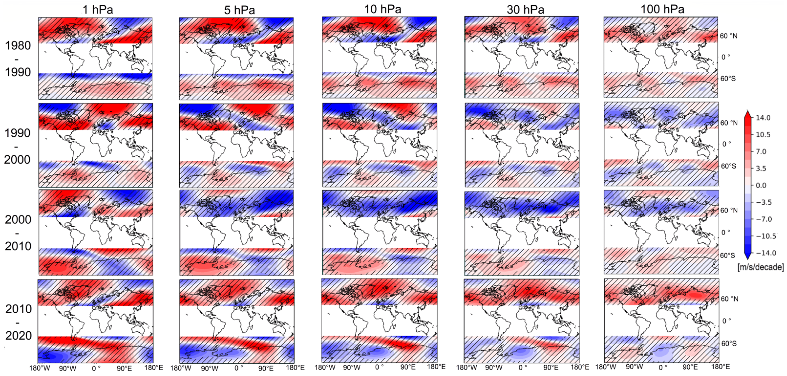
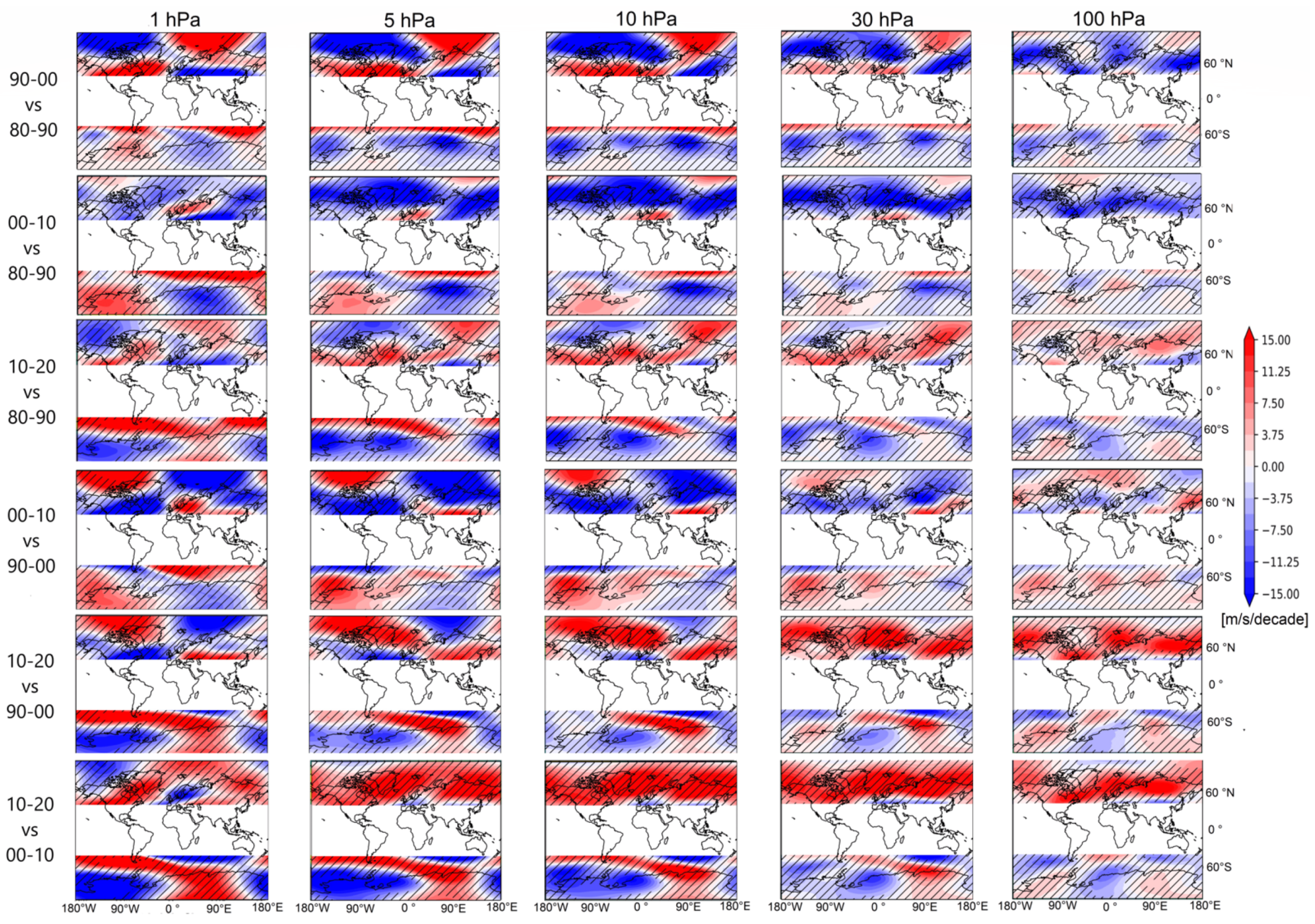
The biggest difference was found between 2000–2010 and 1990–2000 for temperature averages and 2010–2020 and 2000–2010 for temperature trend at 1, 5 and 10 hPa.
(3)
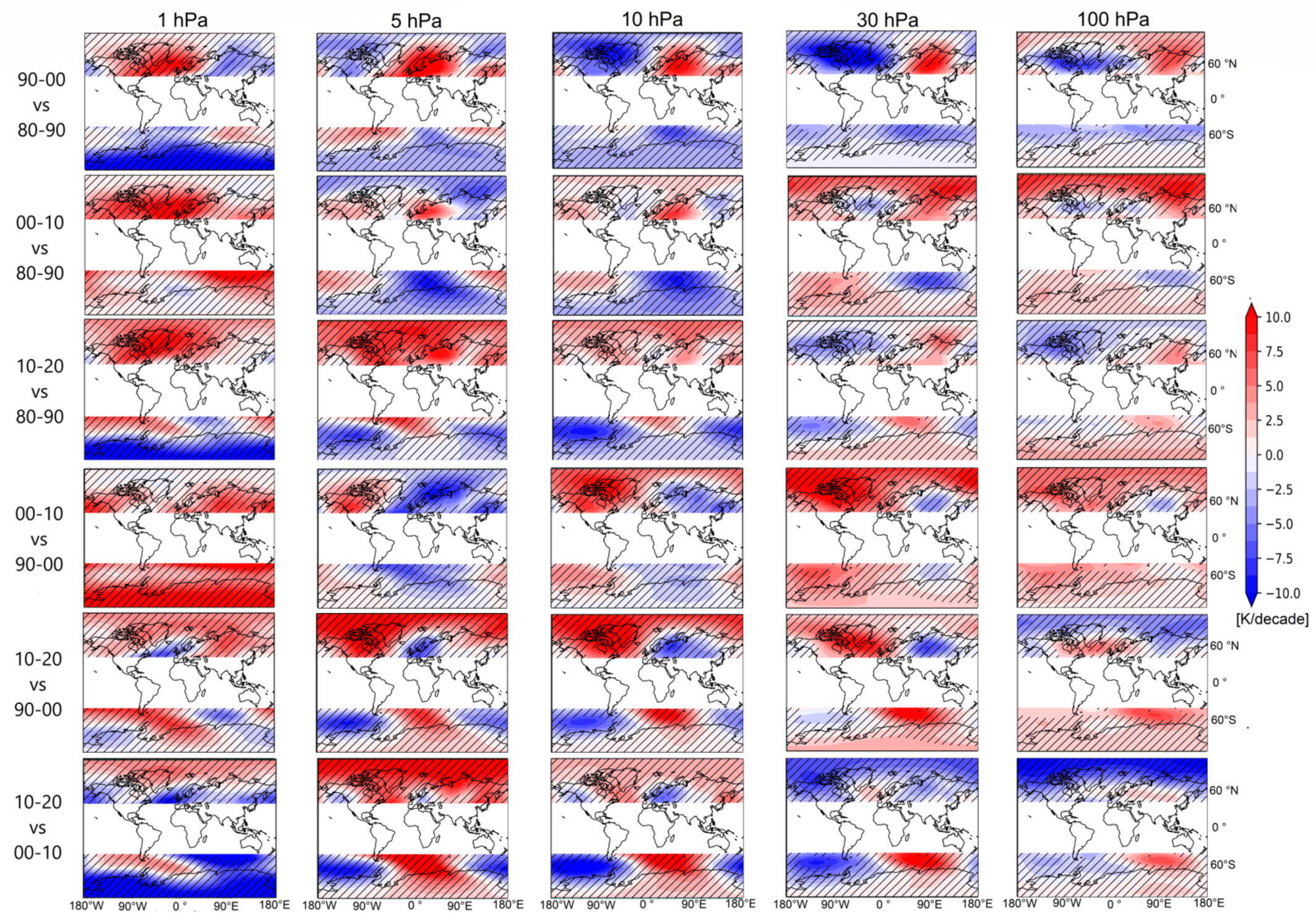
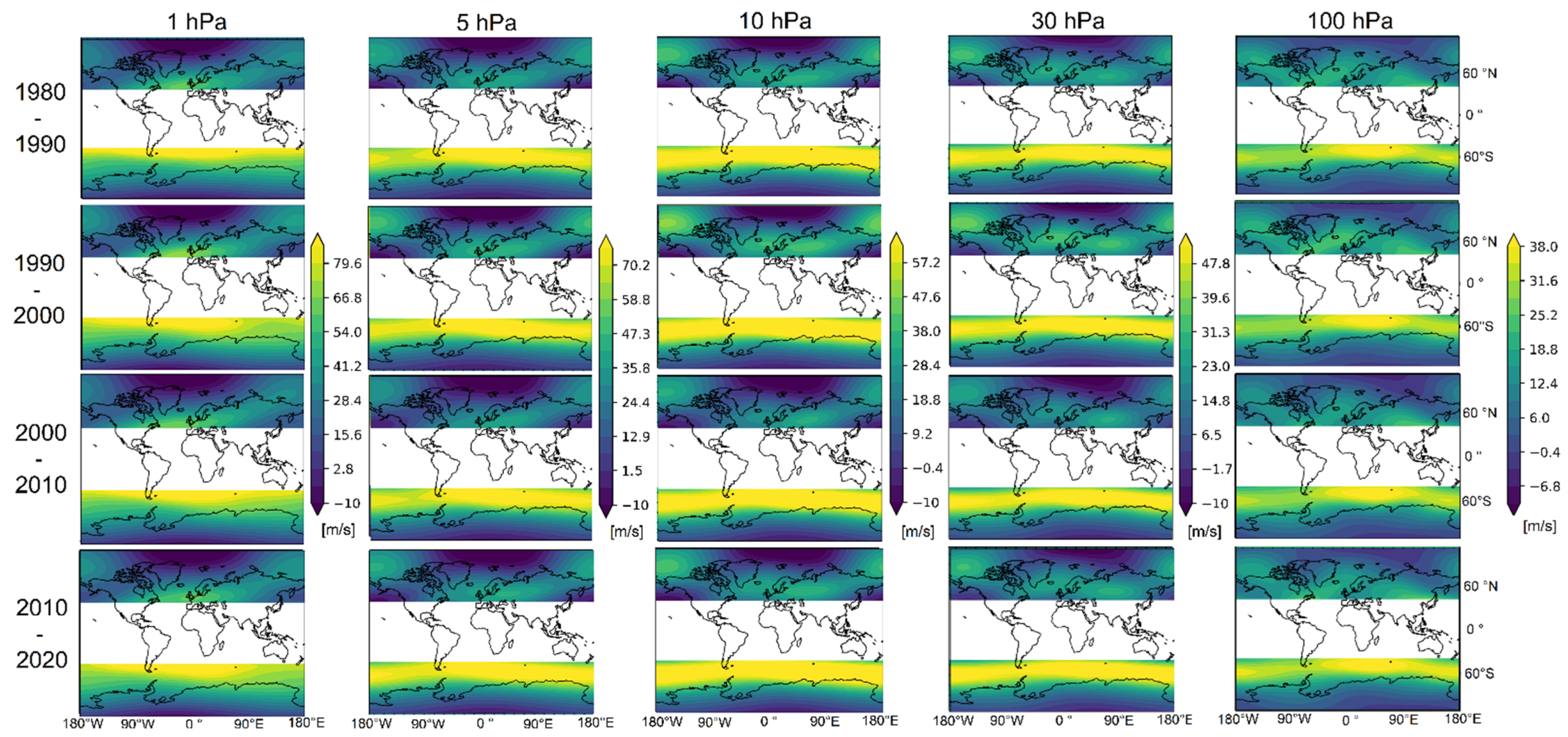
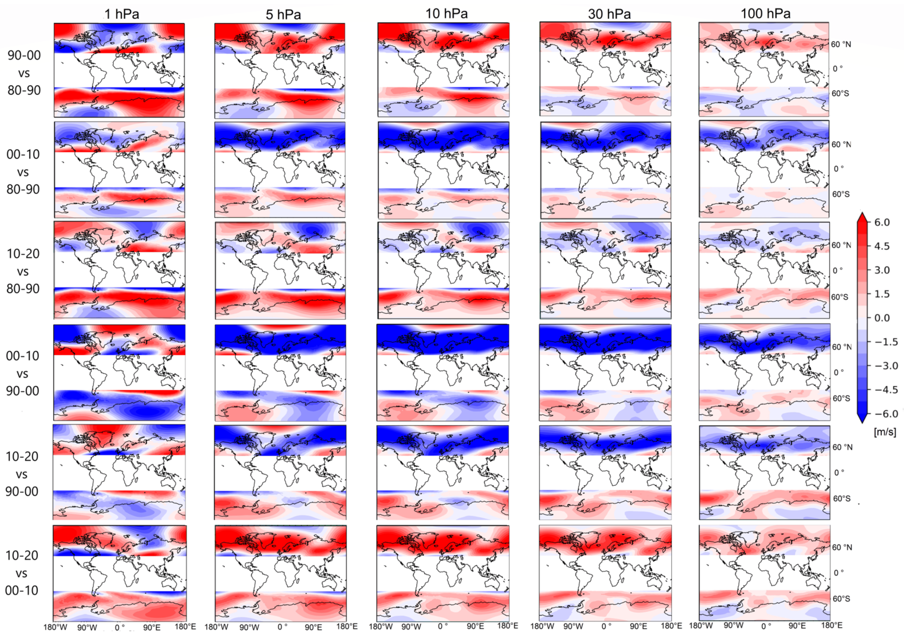
Negative differences occur between 2000–2010 and 1990–2000, and positive differences occur between 1980–1990 and 1990–2000 or 2000–2010 and 2010–2020 for average winds.
(4)
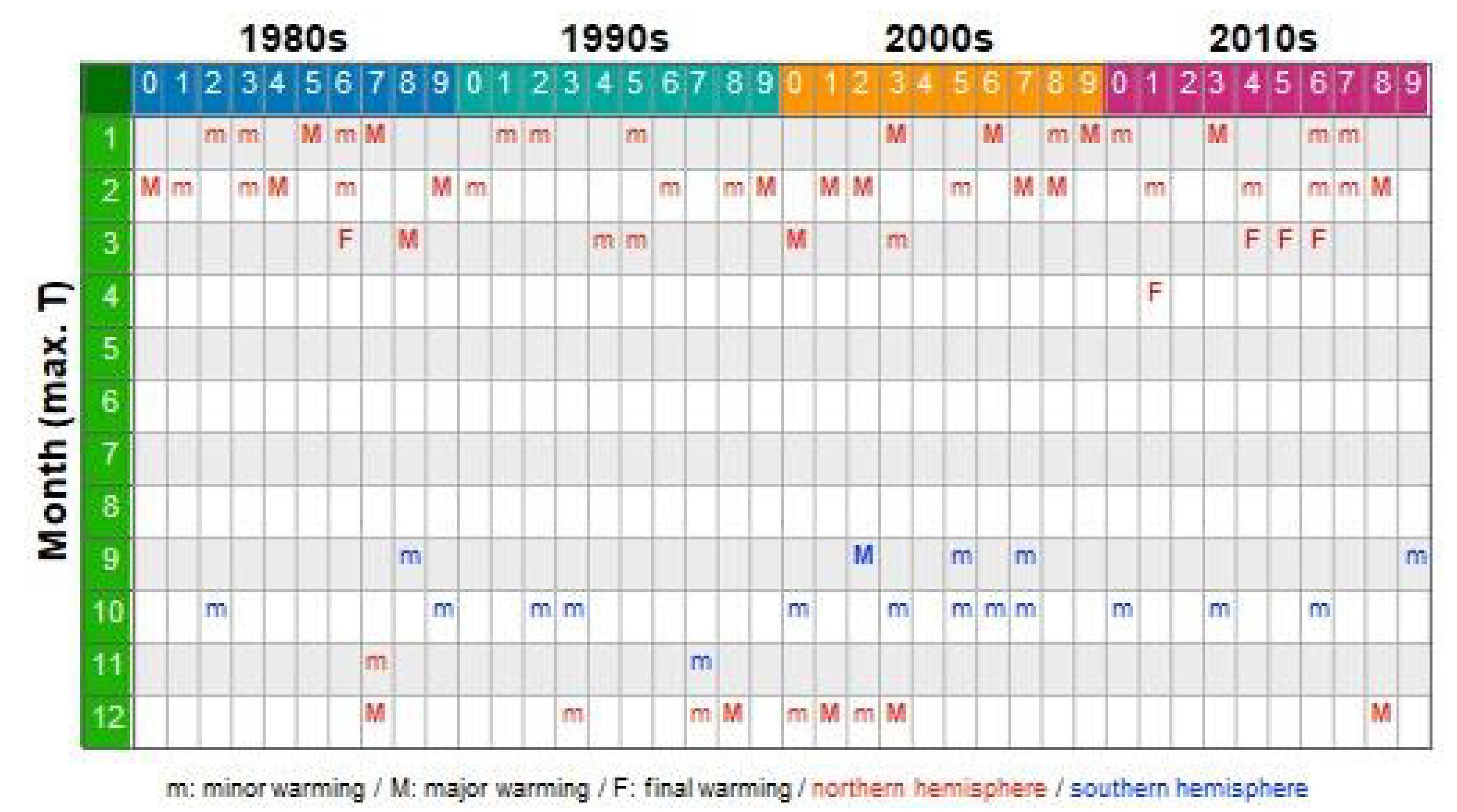
The possible reason for the behavior of climatology is the irregular occurrence of major SSWs in the stratosphere.

Author Contributions

Conceptualization, M.K. and J.L.; methodology, M.K.; validation, M.K. and R.Z.; formal analysis, M.K. and J.L.; investigation, M.K. and R.Z.; resources, M.K.; data curation, R.Z.; writing—original draft preparation, M.K.; writing—review and editing, J.L.; visualization, R.Z.; supervision, M.K.; project administration, J.L.; funding acquisition, J.L. All authors have read and agreed to the published version of the manuscript.

Funding

Support by the Czech Science Foundation via Grant 21-03295S is acknowledged. Part of ERA5 analysis (specifically data homogeneity and climatology analysis) has been funded via LISA–Lidar measurements to Identify Streamers and analyze Atmospheric waves, AEOLUS-INNOVATION, Contract No. 4000133567/20/I-BG ESA project.

Data Availability Statement

Conflicts of Interest

The authors declare no conflict of interest.

References

  1. Steiner, A.; Ladstädter, F.; Randel, W.J.; Maycock, A.C.; Fu, Q.; Claud, C.; Zou, C.Z. Observed Temperature Changes in the Troposphere and Stratosphere from 1979 to 2018. J. Clim. 2020, 33, 8165–8194. [Google Scholar] [CrossRef]
  2. Ramaswamy, V.; Chanin, M.L.; Angell, J.; Barnett, J.; Gaffen, D.; Gelman, M.; Swinbank, R. Stratospheric tem-perature trends: Observations and model simulations. Rev. Geophys. 2001, 39, 71–122. [Google Scholar] [CrossRef]
  3. Jakovlev, A.R.; Smyshlyaev, S.P.; Galin, V.Y. Interannual Variability and Trends in Sea Surface Temperature, Lower and Middle Atmosphere Temperature at Different Latitudes for 1980–2019. Atmosphere 2021, 12, 454. [Google Scholar] [CrossRef]
  4. Huang, F.T.; Mayr, H.G.; Russell, J.M., III; Mlynczak, M.G. Ozone and temperature decadal trends in the stratosphere, mesosphere and lower thermosphere, based on measurements from SABER on TIMED. Ann. Geophys. 2014, 32, 935–949. [Google Scholar] [CrossRef] [Green Version]
  5. Huang, F.T.; Mayr, H.G. Temperature decadal trends, and their relation to diurnal variations in the lower thermosphere, stratosphere, and mesosphere, based on measurements from SABER on TIMED. Ann. Geophys. 2021, 39, 327–339. [Google Scholar] [CrossRef]
  6. Maycock, A.C.; Randel, W.J.; Steiner, A.K.; Karpechko, A.Y.; Christy, J.; Saunders, R.; Thompson, D.W.J.; Zou, C.; Chrysanthou, A.; Abraham, N.L.; et al. Revisiting the Mystery of Recent Stratospheric Temperature Trends. Geophys. Res. Lett. 2018, 45, 9919–9933. [Google Scholar] [CrossRef] [Green Version]
  7. Randel, W.J.; Polvani, L.; Wu, F.; Kinnison, D.E.; Zou, C.-Z.; Mears, C. Troposphere-Stratosphere Temperature Trends Derived From Satellite Data Compared With Ensemble Simulations From WACCM. J. Geophys. Res. Atmos. 2017, 122, 9651–9667. [Google Scholar] [CrossRef]
  8. Rüfenacht, R.; Hocke, K.; Kämpfer, N. First continuous ground-based observations of long period oscillations in the vertically resolved wind field of the stratosphere and mesosphere. Atmos. Chem. Phys. 2016, 16, 4915–4925. [Google Scholar] [CrossRef]
  9. Mitchell, D.M.; Gray, L.; Fujiwara, M.; Hibino, T.; Anstey, J.A.; Ebisuzaki, W.; Harada, Y.; Long, C.; Misios, S.; Stott, P.; et al. Signatures of naturally induced variability in the atmosphere using multiple reanalysis datasets. Q. J. R. Meteorol. Soc. 2014, 141, 2011–2031. [Google Scholar] [CrossRef]
  10. Seppälä, A.; Lu, H.; Clilverd, M.A.; Rodger, C.J. Geomagnetic activity signatures in wintertime stratosphere wind, temperature, and wave response. J. Geophys. Res. Atmos. 2013, 118, 2169–2183. [Google Scholar] [CrossRef] [Green Version]
  11. Butchart, N. The Brewer-Dobson circulation. Rev. Geophys. 2014, 52, 157–184. [Google Scholar] [CrossRef]
  12. Kozubek, M.; Krizan, P.; Lastovicka, J. Northern Hemisphere stratospheric winds in higher midlatitudes: Longitudinal distribution and long-term trends. Atmos. Chem. Phys. 2015, 15, 2203–2213. [Google Scholar] [CrossRef] [Green Version]
  13. Sofieva, V.F.; Szeląg, M.; Tamminen, J.; Kyrölä, E.; Degenstein, D.; Roth, C.; Zawada, D.; Rozanov, A.; Arosio, C.; Burrows, J.P.; et al. Measurement report: Regional trends of stratospheric ozone evaluated using the MErged GRIdded Dataset of Ozone Profiles (MEGRIDOP). Atmos. Chem. Phys. 2021, 21, 6707–6720. [Google Scholar] [CrossRef]
  14. Zhang, Y.; Li, J.; Zhou, L. The Relationship between Polar Vortex and Ozone Depletion in the Antarctic Stratosphere during the Period 1979–2016. Adv. Meteorol. 2017, 2017, 3078079. [Google Scholar] [CrossRef] [Green Version]
  15. Cao, C.; Chen, Y.-H.; Rao, J.; Liu, S.-M.; Li, S.-Y.; Ma, M.-H.; Wang, Y.-B. Statistical Characteristics of Major Sudden Stratospheric Warming Events in CESM1-WACCM: A Comparison with the JRA55 and NCEP/NCAR Reanalyses. Atmosphere 2019, 10, 519. [Google Scholar] [CrossRef] [Green Version]
  16. Charlton, A.J.; Polvani, L.M. A New Look at Stratospheric Sudden Warmings. Part I: Climatology and Modeling Benchmarks. J. Clim. 2007, 20, 449–469. [Google Scholar] [CrossRef]
  17. Baldwin, M.P.; Ayarzagüena, B.; Birner, T.; Butchart, N.; Butler, A.H.; Charlton-Perez, A.J.; Domeisen, D.I.V.; Garfinkel, C.I.; Garny, H.; Gerber, E.P.; et al. Sudden Stratospheric Warmings. Rev. Geophys. 2021, 59, 59. [Google Scholar] [CrossRef]
  18. Holton, J.R.; Tan, H. The Influence of the Equatorial Quasi-Biennial Oscillation on the Global Circulation at 50 mb. J. Atmos. Sci. 1980, 37, 2200–2208. [Google Scholar] [CrossRef] [Green Version]
  19. Coy, L.; Wargan, K.; Molod, A.M.; McCarty, W.R.; Pawson, S. Structure and Dynamics of the Quasi-Biennial Os-cillation in MERRA-2. J. Clim. 2016, 29, 5339–5354. Available online: https://journals.ametsoc.org/view/journals/clim/29/14/jcli-d-15-0809.1 (accessed on 1 October 2021). [CrossRef] [PubMed]
  20. Butchart, N.; Anstey, J.A.; Kawatani, Y.; Osprey, S.M.; Richter, J.H.; Wu, T. QBO Changes in CMIP6 Climate Projections. Geophys. Res. Lett. 2020, 47. [Google Scholar] [CrossRef] [Green Version]
  21. Hersbach, H. The ERA5 global reanalysis. Q. J. R. Meteorol. Soc. 2020, 146, 1999–2049. [Google Scholar] [CrossRef]
  22. Gelaro, R.; McCarty, W.; Suárez, M.J.; Todling, R.; Molod, A.; Takacs, L.; Randles, C.A.; Darmenov, A.; Bosilovich, M.G.; Reichle, R.; et al. The Modern-Era Retrospective Analysis for Research and Applications, Version 2 (MERRA-2). J. Clim. 2017, 30, 5419–5454. [Google Scholar] [CrossRef] [PubMed]
  23. Shao, X.; Ho, S.-P.; Zhang, B.; Cao, C.; Chen, Y. Consistency and Stability of SNPP ATMS Microwave Observations and COSMIC-2 Radio Occultation over Oceans. Remote. Sens. 2021, 13, 3754. [Google Scholar] [CrossRef]
  24. Kursinski, E.G.; Hajj, W.I.; Bertiger, S.S.; Leroy, T.; Meehan, L.; Romans, J.; Schofield, D.; McCleese, W.; Melbourne, C.; Thornton, T.; et al. Initial results of radiooccultation observations of Earth’s atmosphere using the Global Positioning System. Science 1996, 271, 1107–1110. [Google Scholar] [CrossRef]
  25. Jensen, A.S.; Lohmann, M.S.; Benzon, H.-H.; Nielsen, A.S. Full Spectrum Inversion of radio occultation signals. Radio Sci. 2003, 38, 1040. [Google Scholar] [CrossRef]
  26. Kozubek, M.; Krizan, P.; Lastovicka, J. Homogeneity of the Temperature Data Series from ERA5 and MERRA2 and Temperature Trends. Atmosphere 2020, 11, 235. [Google Scholar] [CrossRef] [Green Version]
  27. Fujiwara, M.; Manney, G.L.; Gray, L.J.; Wright, J.S. (Eds.) SPARC Report No. 10, WCRP-6/2021; WCRP: Geneva, Switzerland; Available online: www.sparc-climate.org/publications/sparc-reports (accessed on 9 October 2021). [CrossRef]
  28. Lastovicka, J.; Krizan, P.; Kozubek, M. Longitudinal structure of stationary planetary waves in the middle atmosphere–extraordinary years. Ann. Geophys. 2018, 36, 181–192. [Google Scholar] [CrossRef] [Green Version]
  29. Shangguan, M.; Wang, W.; Jin, S. Variability of temperature and ozone in the upper troposphere and lower stratosphere from multi-satellite observations and reanalysis data. Atmos. Chem. Phys. 2019, 19, 6659–6679. [Google Scholar] [CrossRef] [Green Version]
  30. Diallo, M.; Ern, M.; Ploeger, F. The advective Brewer–Dobson circulation in the ERA5 reanalysis: Climatology, variability, and trends. Atmos. Chem. Phys. 2021, 21, 7515–7544. [Google Scholar] [CrossRef]
  31. Rüfenacht, R.; Murk, A.; Kampfer, N.; Eriksson, P.; Buehler, S.A. Middle-atmospheric zonal and meridional wind profiles from polar, tropical and midlatitudes with the ground-based microwave Doppler wind radiometer WIRA. Atmos. Meas. Tech. 2014, 7, 4491–4505. [Google Scholar] [CrossRef] [Green Version]
  32. Baldwin, M.P.; Gray, L.J.; Dunkerton, T.J.; Hamilton, K.; Haynes, P.H.; Randel, W.J.; Takahashi, M. The quasi-biennial oscillation. Rev. Geophy. 2001, 39, 179–229. [Google Scholar] [CrossRef]
  33. Osprey, S.M.; Butchart, N.; Knight, J.R.; Scaife, A.A.; Hamilton, K.; Anstey, J.A.; Zhang, C. An unexpected dis-ruption of the atmospheric quasi-biennial oscillation. Science 2016, 353, 1424–1427. [Google Scholar] [CrossRef] [PubMed] [Green Version]
  34. Clette, F. Is the F10.7cm–Sunspot Number relation linear and stable? J. Space Weather. Space Clim. 2021, 11, 2. [Google Scholar] [CrossRef]
  35. WMO CAS. Abridged Final Report of the Seventh Session, Manila, 27 February, Midlatitudes with the Ground-Based Microwave Doppler Wind Radiosonde. 1978. Available online: https://library.wmo.int/index.php?lvl=notice_display&id=8938#.YaojAtpBw2w (accessed on 9 October 2021).
  36. Kozubek, M.; Lastovicka, J.; Krizan, P. Comparison of Key Characteristics of Remarkable SSW Events in the Southern and Northern Hemisphere. Atmosphere 2020, 11, 1063. [Google Scholar] [CrossRef]
Figure 1. Temperature climatology (upper panels) and trends (lower panels) for January during 1980–2020 at 1, 10, 50 and 100 hPa using ERA5 and MERRA-2.
Remotesensing 13 04923 g001
Figure 2. Temperature climatology (K) for 1980–1990, 1990–2000, 2000–2010 and 2010–2020 using ERA5 reanalysis at 1, 5, 10, 30 and 100 hPa.
Remotesensing 13 04923 g002
Figure 3. Difference of temperature climatology (K) between decades for 1, 5, 10, 30 and 100 hPa using ERA5 reanalysis.
Remotesensing 13 04923 g003
Figure 4. Temperature trend (K/dec) for 1980–1990, 1990–2000, 2000–2010 and 2010–2020 using ERA5 reanalysis at 1, 5, 10, 30 and 100 hPa.
Remotesensing 13 04923 g004
Figure 5. Difference of temperature trend (K) between decades for 1, 5, 10, 30 and 100 hPa using ERA5 reanalysis.
Remotesensing 13 04923 g005
Figure 6. Zonal wind climatology (m/s, blue means westerly, yellow easterly wind) for 1980–1990, 1990–2000, 2000–2010 and 2010–2020 using ERA5 reanalysis at 1, 5, 10, 30 and 100 hPa.
Remotesensing 13 04923 g006
Figure 7. Difference of zonal wind climatology (m/s) between decades for 1, 5, 10, 30 and 100 hPa using ERA5 reanalysis.
Remotesensing 13 04923 g007
Figure 8. Zonal wind trend (m/s/dec) for 1980–1990, 1990–2000, 2000–2010 and 2010–2020 using ERA5 reanalysis at 1, 5, 10, 30 and 100 hPa.
Remotesensing 13 04923 g008
Figure 9. Difference of zonal wind trend (m/s) between decades for 1, 5, 10, 30 and 100 hPa using ERA5 reanalysis.
Remotesensing 13 04923 g009
Figure 10. Time series of NAO, ENSO, F10.7 cm, and QBO at 10 and 50 hPa for period 1970–2019.
Remotesensing 13 04923 g010
Figure 11. Occurrence of the SSW on the NH and SH. Capital letter means major SSW according to WMO definition.
Remotesensing 13 04923 g011
Publisher’s Note: MDPI stays neutral with regard to jurisdictional claims in published maps and institutional affiliations.

