Article

Evaluation of foF2 and hmF2 Parameters of IRI-2016 Model in Different Latitudes over China under High and Low Solar Activity Years

1
School of Geographic Sciences, Xinyang Normal University, Xinyang 464000, China
2
School of Geodesy and Geomatics, Wuhan University, Wuhan 430079, China
3
School of Environmental Science and Spatial Informatics, China University of Mining and Technology, Xuzhou 221116, China
*
Author to whom correspondence should be addressed.
Remote Sens. 2022, 14(4), 860; https://doi.org/10.3390/rs14040860
Submission received: 15 January 2022 / Revised: 9 February 2022 / Accepted: 10 February 2022 / Published: 11 February 2022
(This article belongs to the Special Issue GNSS Atmospheric Modelling)

Abstract

:
The height of the peak electron density (hmF2) and the critical frequency of the F2 layer (foF2) are very important in the research of ionospheric electrodynamics and high frequency (HF) wireless communication. In the article, we validated the hmF2/foF2 model values of the latest version of the International Reference Ionosphere (IRI-2016) with observations from three ionosonde stations which belong to low, middle, and high latitudes (i.e., Sanya, Beijing and Mohe) over China during a high solar activity year (2014, F10.7 = 145.9 sfu) and a low solar activity year (2016, F10.7 = 88.7 sfu). Among them, foF2 model values can be obtained through the International Radio Consulting Committee (CCIR) model or the International Union of Radio Science (URSI) model, both of which have the “F-peak storm model” on or ‘off’ options; hmF2 model values can be obtained through Bilitza-Sheikh-Eyfrig (BSE-1979), Altadill-Magdaleno-Torta-Blanch (AMTB-2013), or SHUbin (SHU-2015) model. The IRI-2016 hmF2/foF2 model values were evaluated by root mean square (RMS) values and mean absolute relative error (MARE). The results show that for the foF2 parameter, the performance of IRI-2016 can be improved by choosing “F-peak storm model” on option in geomagnetic-disturbed days. Whether in high or low solar activity years, for foF2, the IRI-2016 options of CCIR have better prediction ability than IRI-2016 options of URSI in low and high latitudes over China, and the IRI-2016 options of URSI have better prediction ability than IRI-2016 options of URSI in middle latitudes. For hmF2, the IRI-2016 option of SHU-2015 has better prediction ability than the IRI-2016 options of AMTB-2013 and BSE-1949 in high latitudes over China, the IRI-2016 options of SHU-2015 and BSE-1979 have better prediction ability than IRI-2016 options of AMTB-2013 in mid and low latitudes over China.

1. Introduction

Modern short-wave communication is widely used in various fields of production and life. For example, global navigation satellite systems (GNSS), through short wave positioning and communication, are widely used in the world, especially in the military. Its mobility, survivability and long-distance communication capability have not only become one of the important means of international communication and global communication, but also attracted more and more attention in the field of short-range communications, such as emergency and counter-terrorism, in recent years. The height of the peak electron density (hmF2) and the critical frequency of the F2 layer (foF2) are very important for short wave communication, especially for short wave NVIS (near vertical incident sky-wave) communication. Their changes will directly affect the selection and design of parameters such as the radio wave radiation elevation and the working frequency band in short wave communication lines, and then affect the distance and efficiency of communication.
In recent years, researchers have made several efforts to improve the modelling and forecasting capability of the foF2 and hmF2 parameters, and other relevant ionospheric parameters. For most radio propagation applications, the values of hmF2 and foF2 are of great importance [1]. So far, the International Reference Ionosphere (IRI) [2,3] is the most widely used by the ionospheric community as the standard model of the ionosphere. The IRI model is calculated by using ground multi-source observations and spaceborne satellite observations [4,5]. The IRI model can be optimized by GNSS-TEC to establish a virtual ionosonde. Thus, hmF2 and foF2 can be effectively estimated anywhere and anytime to meet the communication requirements of high-frequency signals [6]. With the enrichment of GNSS observations and the optimization of algorithms, the IRI model has been improved continuously, and substantive progress has been made.
What is more, relevant scholars at home and abroad have carried out a series of fruitful research work using the IRI model and achieved a series of scientific research results. With the diversification of observations and the continuous optimization of algorithms, the IRI model is also improving. In order to better predict foF2 and hmF2 accurately, some scholars have studied foF2/hmF2 modeling and accuracy evaluation using multi-source data [7,8,9,10,11,12,13], meanwhile, relevant scholars have studied the adaptability analysis of IRI hmF2/foF2 under different geomagnetic activities in different research areas. Some scholars have studied the adaptability of IRI model in different latitudes with ionosonde data [14,15,16,17,18,19,20]. Some scholars have also studied the adaptability analysis of F2 parameters and improved methods of IRI model during different geomagnetic storms [21,22,23,24,25]. There have also been studies of the F2 parameters’ adaptability of different IRI models in high and low solar activity years [26,27,28,29,30,31]. Research has also focused on the foF2 applicability analysis of the IRI model over China [32,33,34]. Compared to the earlier versions of IRI (e.g., IRI-2007 [3] and IRI-2012 [8]), the latest version of international reference ionosphere (IRI-2016) [1] has been greatly improved. Until now, on the one hand, IRI-2016 contains three options for hmF2, which are Bilitza–Sheikh–Eyfrig (BSE-1979) [
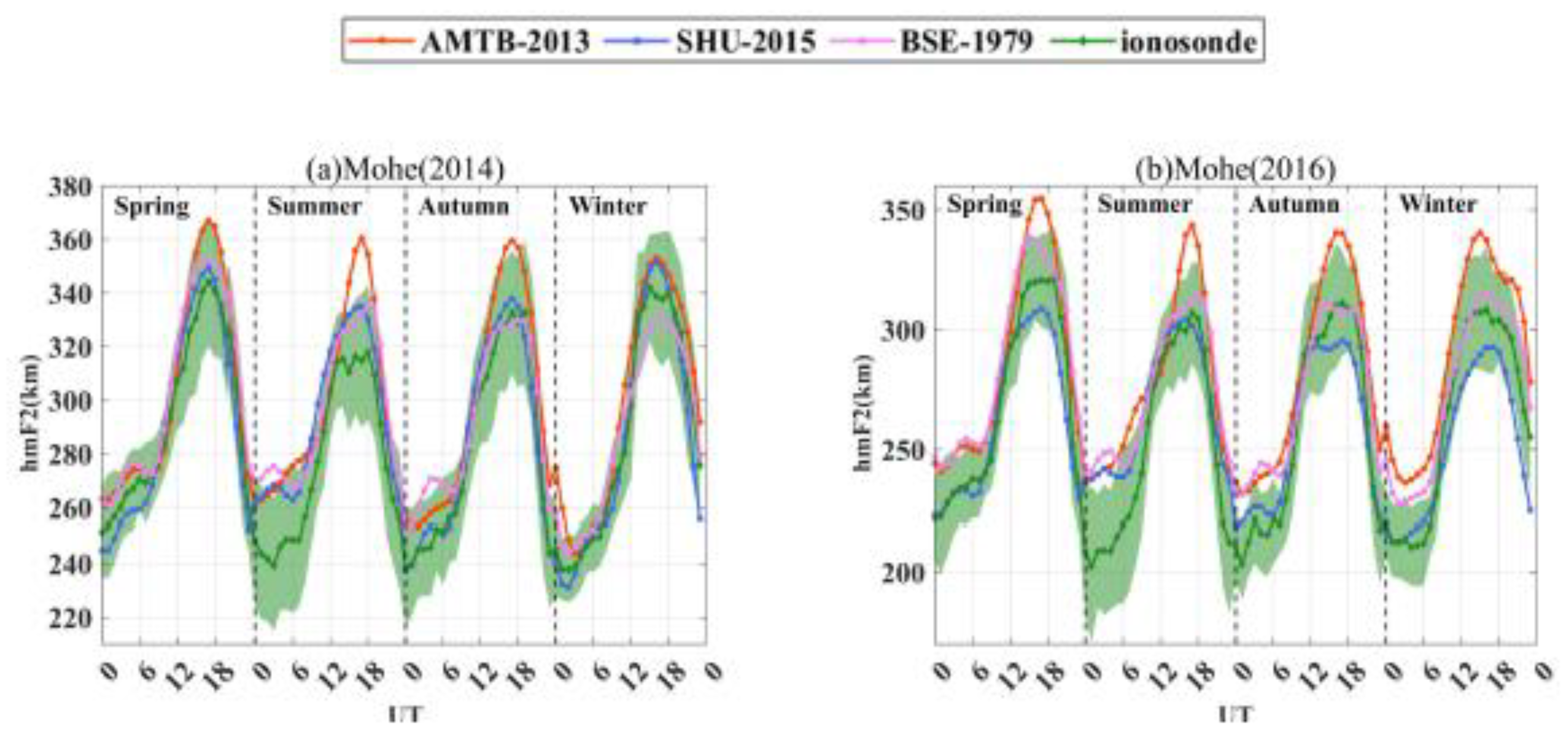
9], Altadill–Magdaleno–Torta-Blanch (AMTB-2013) [7] and Shubin (SHU-2015) [13]. On the other hand, IRI-2016 offers two modes for foF2, which are the International Radio Consulting Committee (CCIR) [35] and the International Union of Radio Science (URSI) [19], both of which have the “F-peak storm model” ‘on’ or ‘off’ options. The BSE-1979 model was proposed by Bilitza et al. in 1979 [9]. The model depends not only on the correlation between M(3000)F2 and hmF2, but also on the number of sunspots (R12) in 12 months. The AMTB-2013 model was calculated based on the 26 ionosonde observations during geomagnetic calm period from years 1998 to 2006 [7]. Finally, the SHU-2015 model is obtained from the ionospheric radio occultation data of CHAMP (Challenging Minisatellite Payload) (years 2001 to 2008), GRACE (Gravity Recovery and Climate Experiment) (years 2007 to 2011) and COSMIC (Constellation Observing System for Meteorology, Ionosphere and Climate) (years 2006 to 2012) and the 62 ionosonde observations in the world from the years 1987 to 2012 [13]. The main advantage of the new IRI model is that it can directly predict hmF2 instead of using its relationship with M(3000)F2 [1]. These options provide an opportunity for the users to evaluate hmF2 and foF2 model values and compare them with other data sets in order to provide valuable feedback on uncertainty and differences from real hmF2 and foF2 values. This is necessary for improving model accuracy and measurement technology [1]. Given the importance of foF2 and hmF2 parameters, mastering the IRI-2016 daily variations for foF2 and hmF2 is of great significance to effectively realize short wave communication (e.g., BeiDou Navigation Satellite System, (BDS)) under various conditions over China.
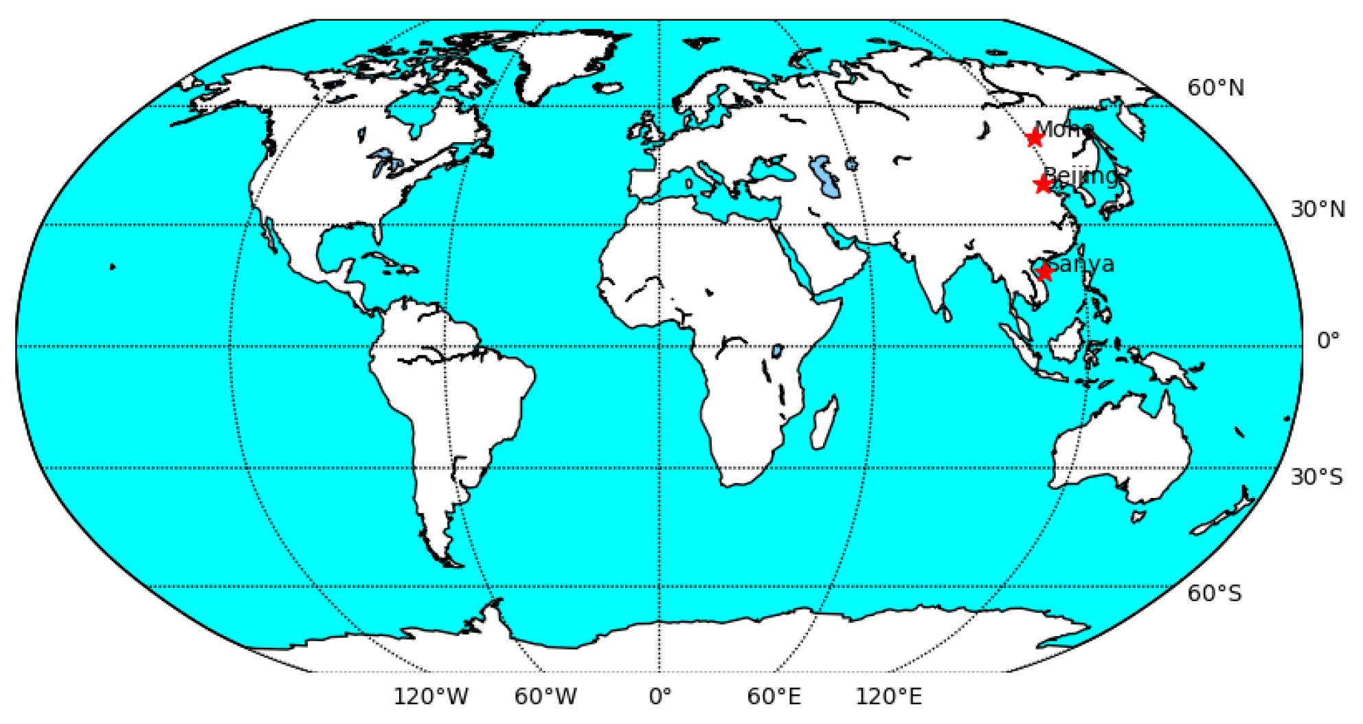
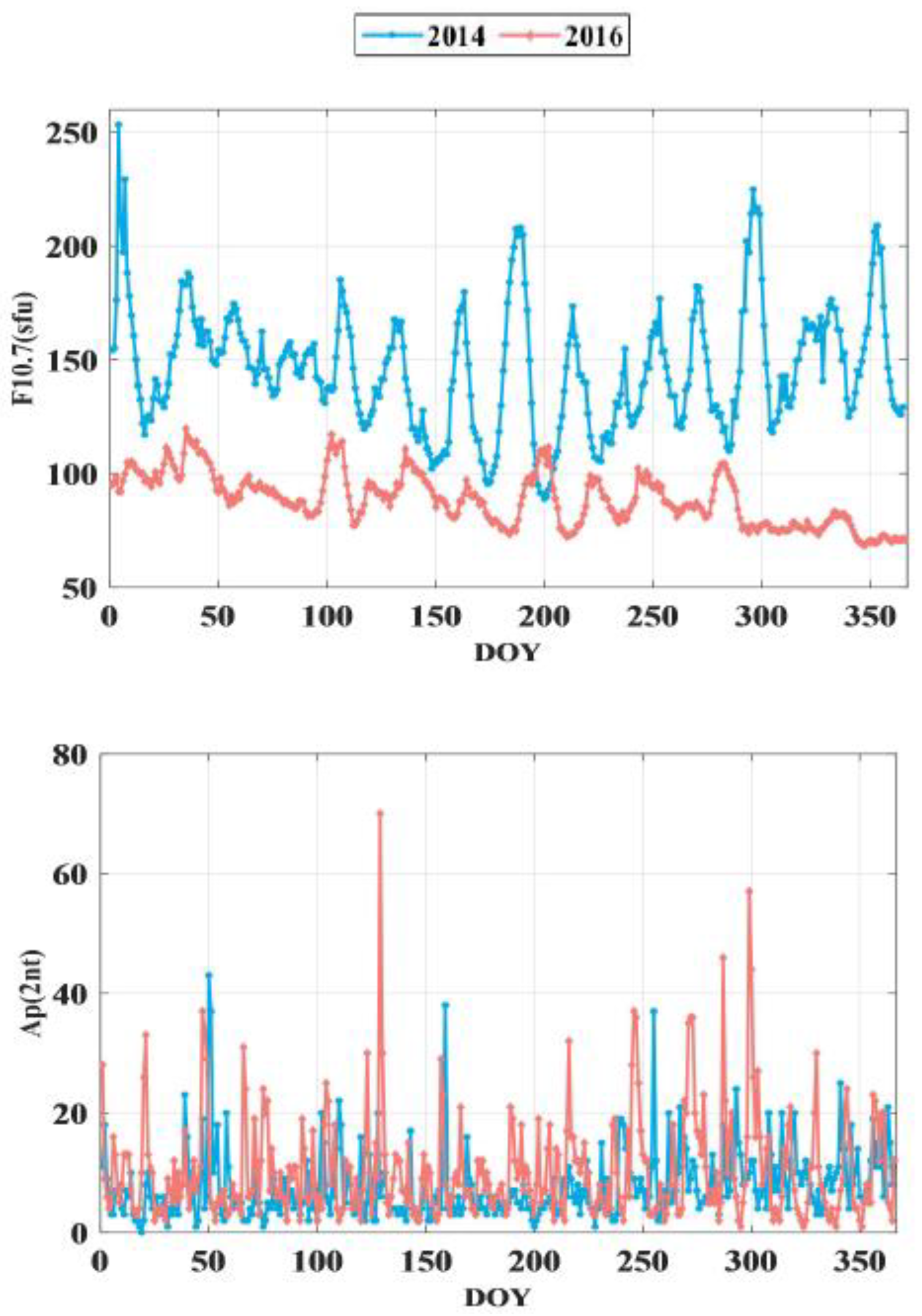
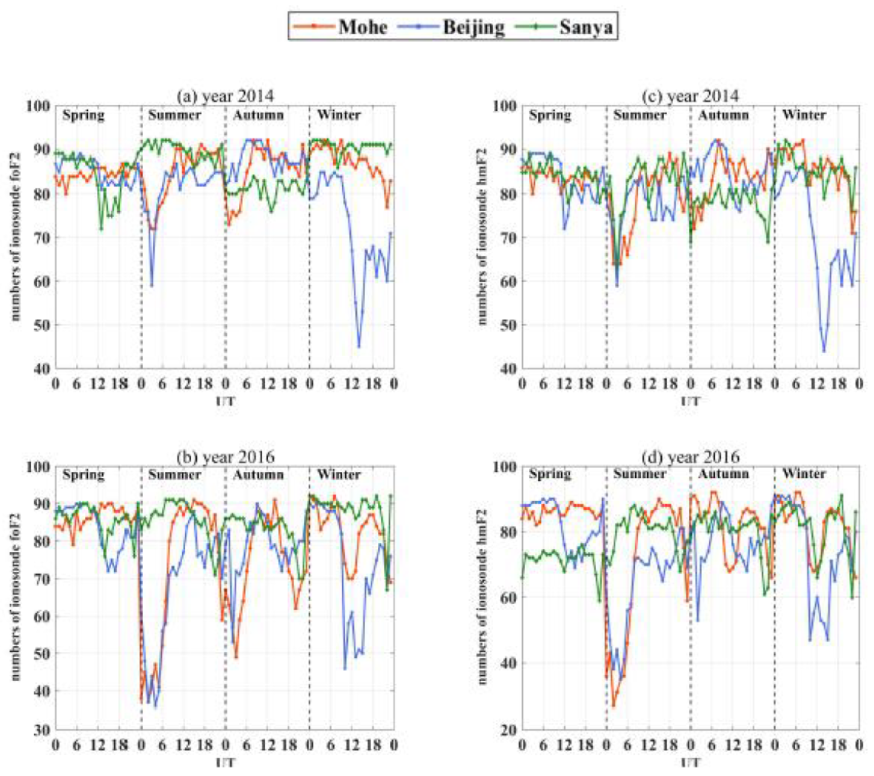
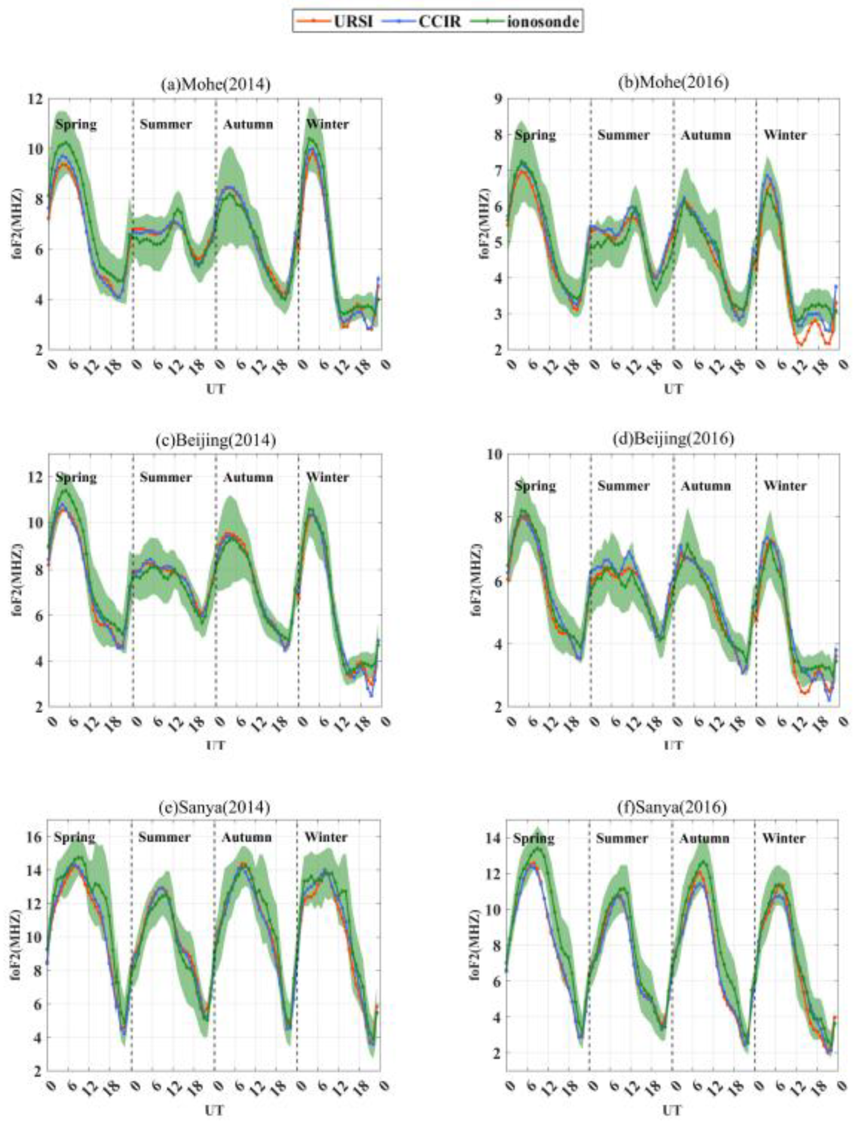
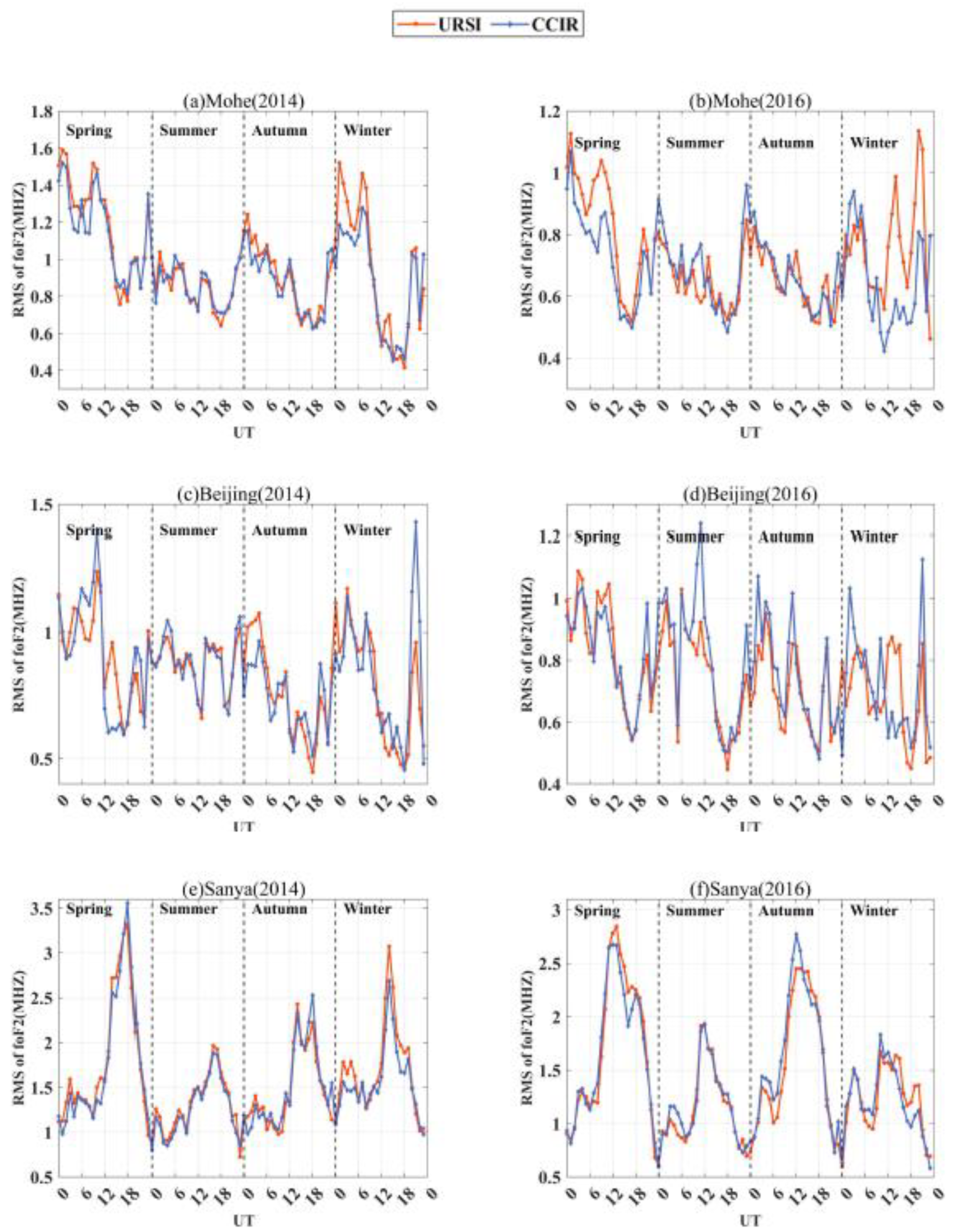
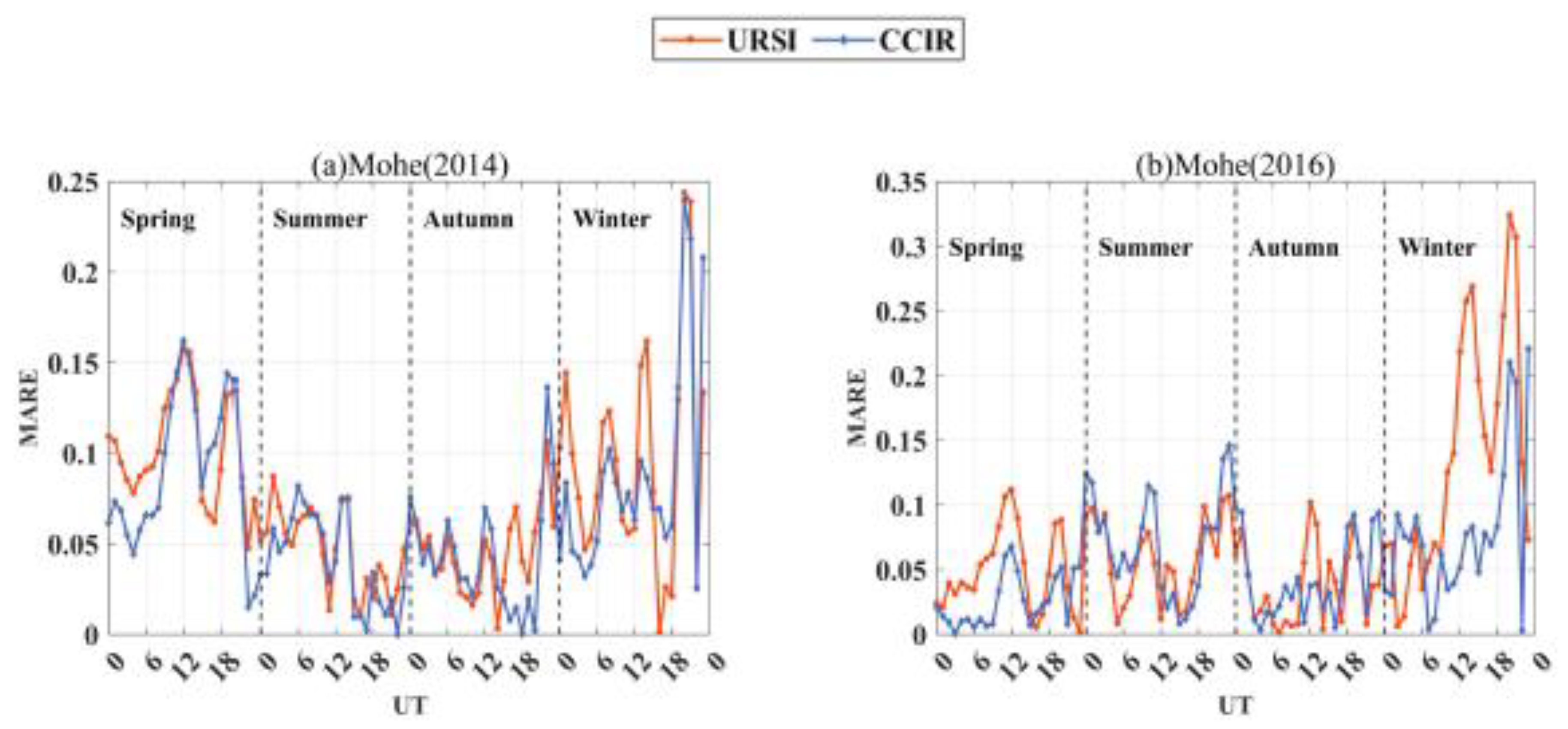
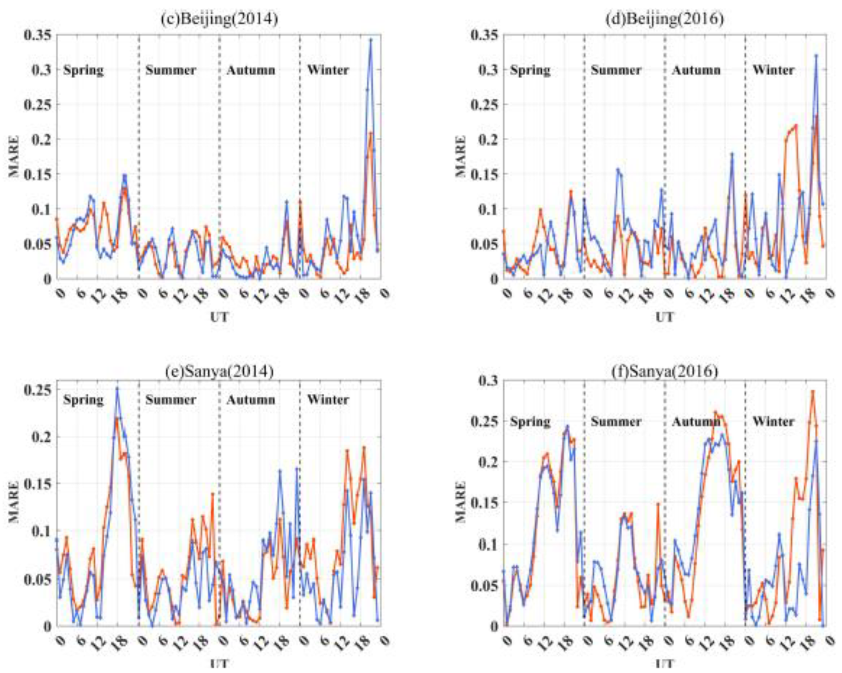
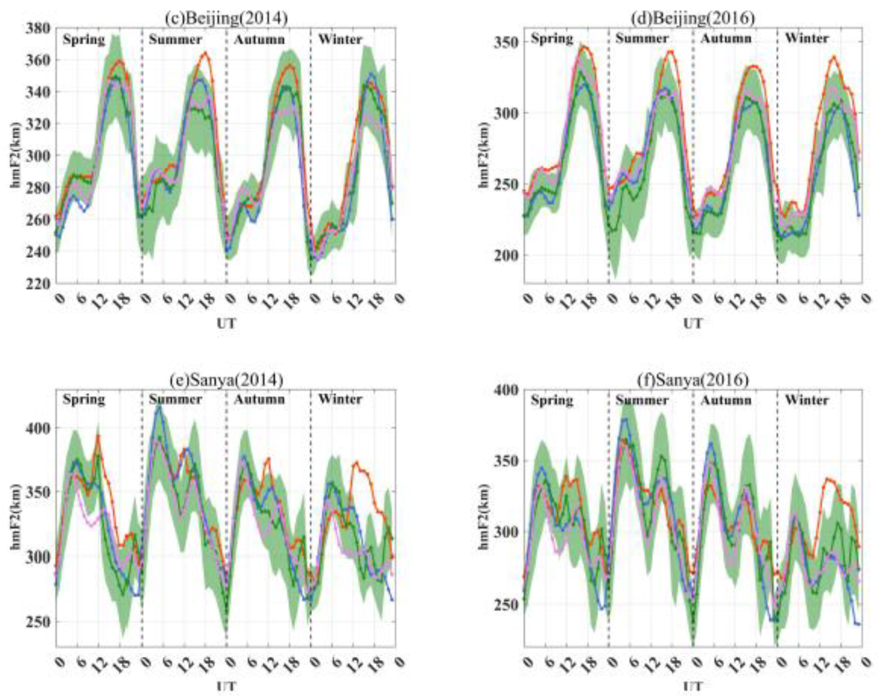
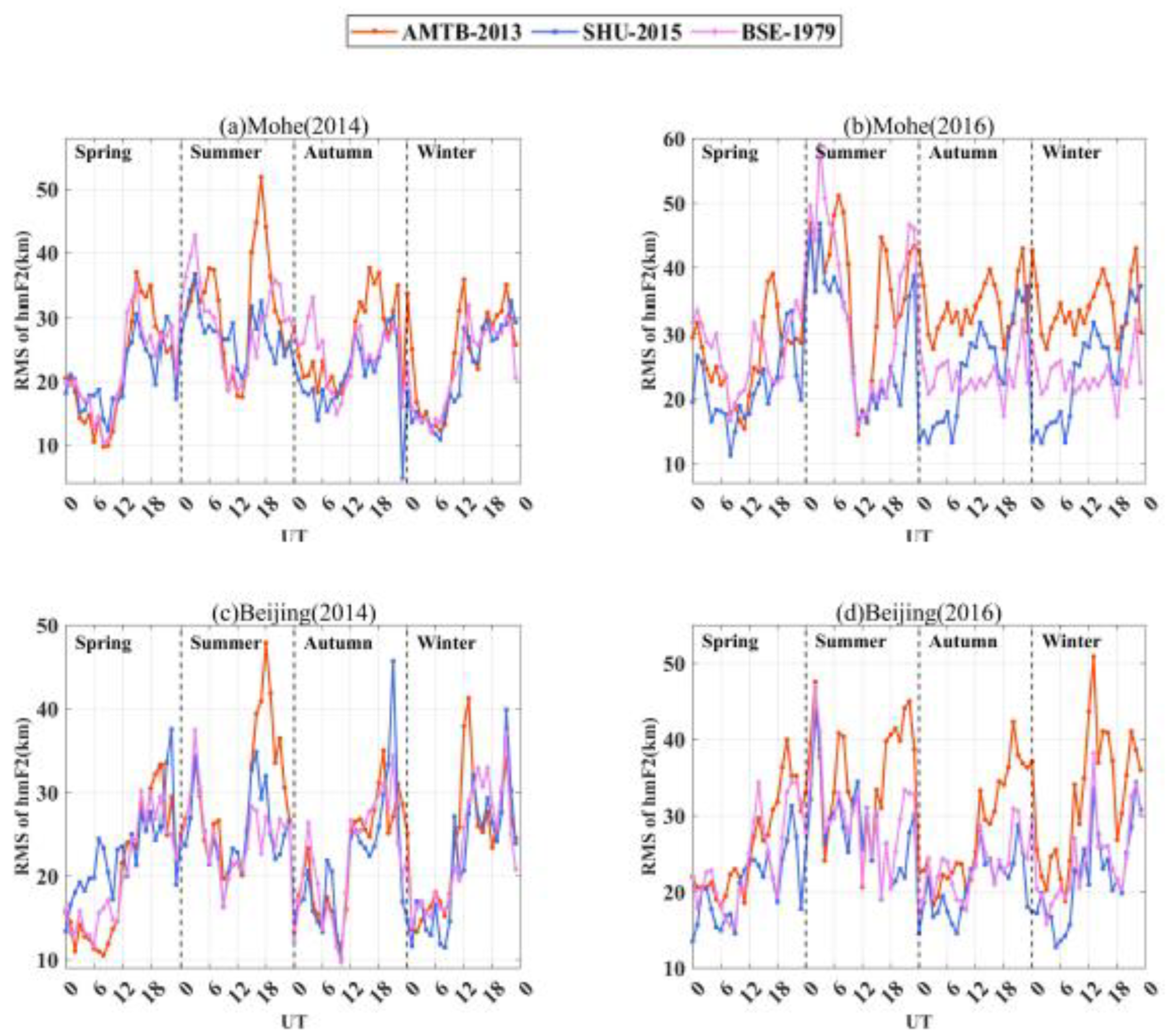
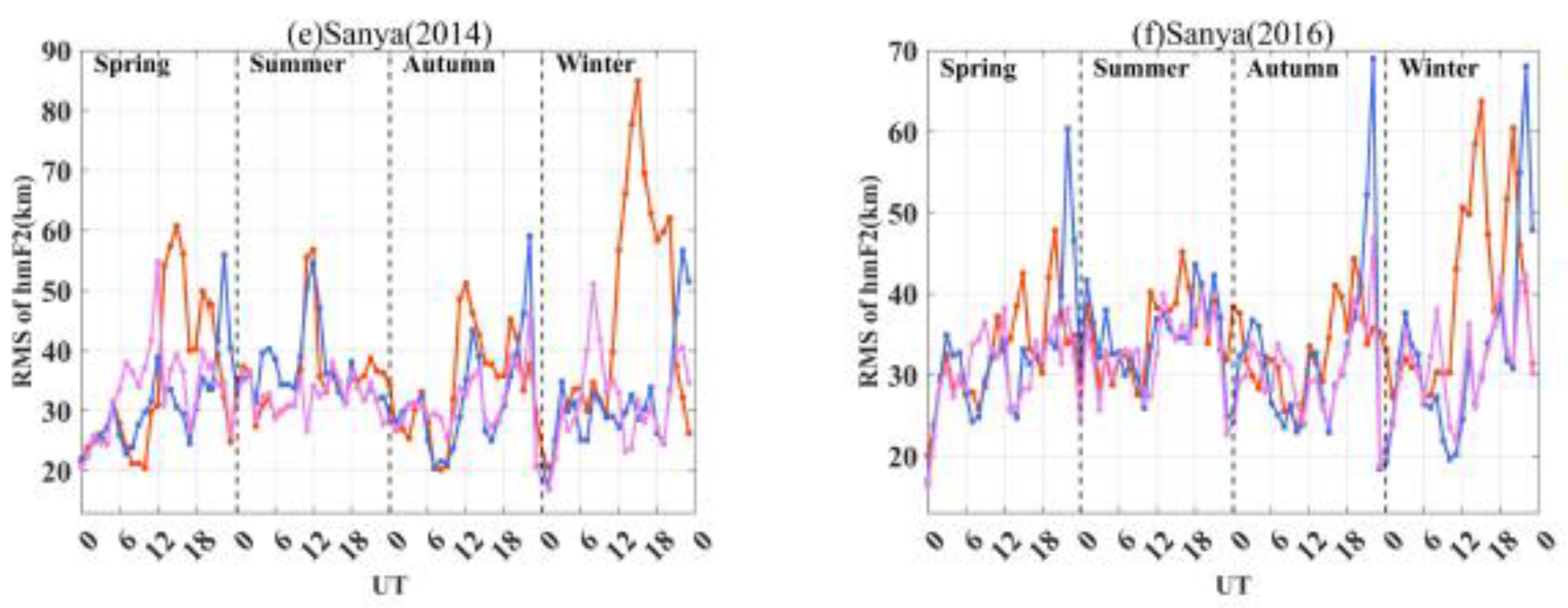
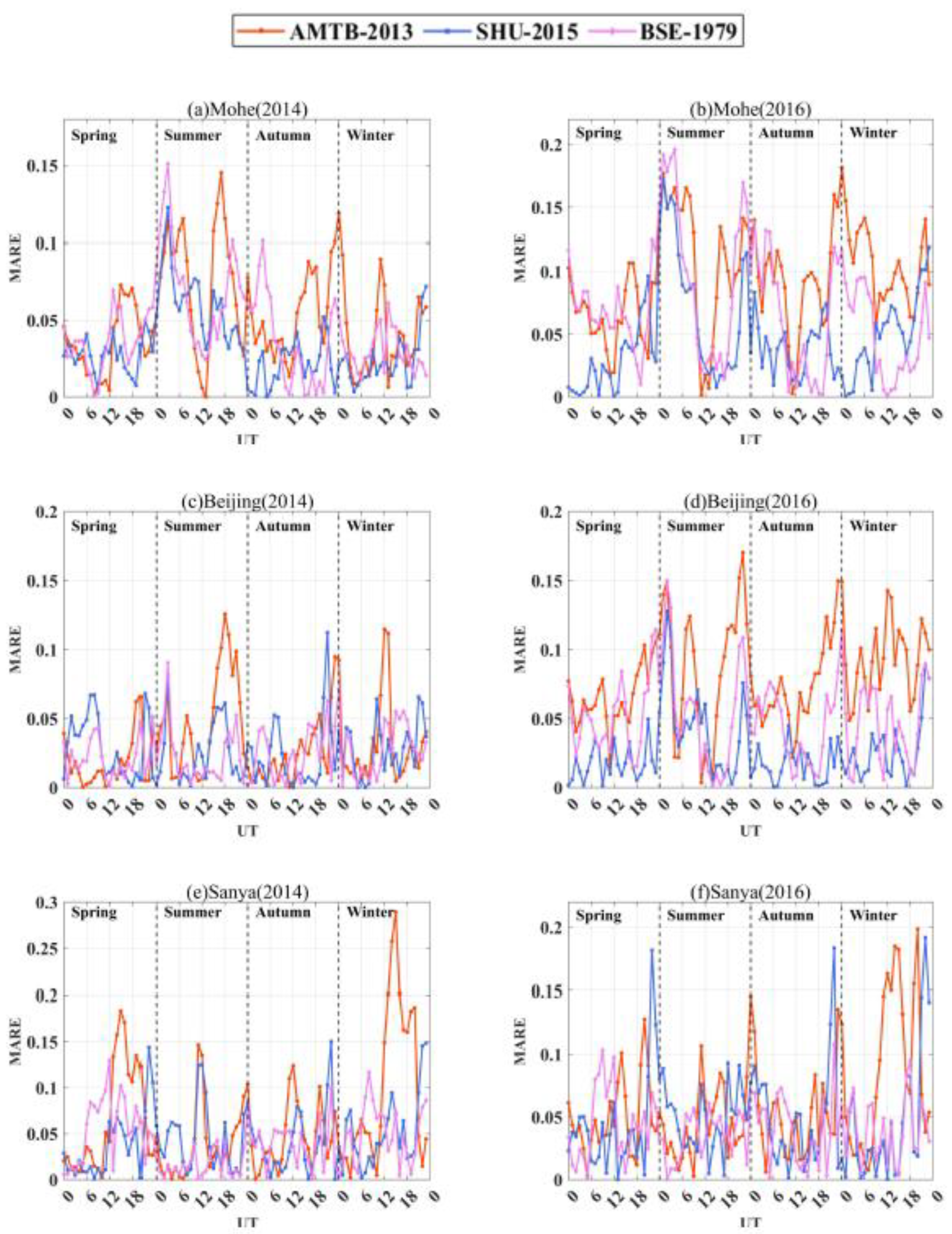
This paper determines which option performs best under low and high solar activity years, by evaluating the different IRI-2016 hmF2 and foF2 model options with ionosonde data in low, middle and high latitudes over China. In order to accomplish this task, we considered the ionosonde stations of Sanya (Geog.18.34°N, 109.42°E and Geom.8.87°N, 177.99°W), Beijing (Geog.40.30°N, 116.20°E and Geom.30.85°N, 172.10°W) and Mohe (Geog.52.00°N, 122.52°E and 42.73°N, 167.26°W) over China, as shown in Figure 1. This paper is organized as follows: Section 2 shows the materials and methods used, and Section 3 evaluates IRI-2016 model performance of foF2 and hmF2 data by root mean square (RMS) values and mean absolute relative error (MARE). Finally, Section 4 and Section 5 give the discussion and conclusion.

2. Materials and Methods

2.1. Materials

In this study, both model and observational datasets were used. The model data include predictions from the three IRI-2016 hmF2 model options and four IRI-2016 foF2 model options. The observational data of hmF2 and foF2 values come from different latitude ionosonde stations over China. The datasets cover periods under low solar activity year (2016) and high solar activity year (2014) during the 24th solar cycle. The ionosonde observations are from Sanya, Beijing and Mohe over China. Figure 1 presents the three ionosonde stations considered in the study. Figure 2 presents the variation of the daily F10.7 solar indice (top) and Ap index (below) for the years 2014 and 2016. As shown in Figure 1, Sanya, Beijing and Mohe belong to geographical low, middle and high latitudes over China, respectively. The ionosonde data were provided by the Global Ionospheric Radio Observatory (GIRO), that is hosting the Digital Ionogram DataBase (DIDB), available via http://ulcar.uml.edu/DIDBase (accessed on 1 December 2021). The resampling interval of the ionosonde stations is one hour at all the stations.
The IRI-2016 model was used in this study. The IRI-2016 model is available online at https://ccmc.gsfc.nasa.gov/modelweb/models/iri2016_vitmo.php (accessed on 8 December 2021). In order to evaluate the hmF2/foF2 options with ionosonde observations, the model values in this study are obtained by running IRI-2016 under a given year, date, time, geographic (magnetic) latitude and longitude conditions, in which the hmF2 model values can be obtained by modes of BSE-1979, AMTB-2013 and SHU-2015.
The foF2 model values can be obtained through CCIR mode or URSI mode, and both modes have the option of ”F-peak storm model” ‘on’ or ‘off’, namely CCIR storm ‘on’, CCIR storm ‘off’, URSI storm ‘on’, URSI storm ‘off’. In order to study the influence of “F-peak storm model” ‘on’ or ‘off’ on the predicted value of foF2 in geomagnetic disturbed or geomagnetic quiet period, we have conducted corresponding evaluation tests, as shown below.
Firstly, the data of the geomagnetic quiet period and the geomagnetic disturbed period are classified and compared with the help of the geomagnetic index. There are many indices describing geomagnetic activity, including the Kp, Ap and Dst indices. Among them, the Ap index, called the planetary equivalent daily amplitude index, is the global all-day geomagnetic disturbance intensity index, which can be used as a measure of the level of magnetic activity in the world. In the study of ionosphere, the Ap index is often used to describe the activity state of geomagnetism. Generally, the Ap index used was obtained from the National Aeronautics and Space Administration (NASA), on the site https://omniweb.Gsfc.nasa.gov/form/dx1.html (accessed on 1 December 2021). The data refer to the years 2014 and 2016, and the days with Ap < 30 nT were considered as quiet geomagnetic days [36], while the days with higher Ap values were considered disturbed days. The number of ionosonde measurements at quiet and disturbed geomagnetic periods, at each station, are in Table 1.
Secondly, the RMS value is used to evaluate the prediction performance of IRI-2016 foF2 parameters when the “F-peak storm model” is ‘on’ or ‘off’. We chose the foF2 ionosonde measured as the reference value and compared the differences between IRI-2016 predicted foF2 and foF2 ionosonde measured. Then we calculated RMS values of foF2 in geomagnetic disturbed days and geomagnetic quiet days, respectively, according to the Formula (1), as shown in Table 2. It can be seen from Table 2 that for the IRI-2016 URSI and CCIR options, the prediction ability of the “F-peak storm model” ‘on’ option and the “F-peak storm model” ‘off’ option are basically the same on geomagnetic quiet days, and the prediction accuracy of “F-peak storm model” ‘on’ option is better than that of “F-peak storm model” ‘off’ option on disturbed days. Compared with the “F-peak storm model” ‘off’ option, the prediction accuracy of “F-peak storm model” ‘on’ option is improved by about 10% in Mohe and Beijing, and about 5% in Sanya.
Lastly, in view of the excellent performance of the “F-peak storm model” ‘on’ option, in subsequent studies, whether in CCIR mode or URSI mode of IRI-2016, the default option of “F-peak storm model” in IRI-2016 was on.
The seasonal analysis considered Spring as the months February, March and April; Summer as May, June and July; Autumn as August, September and October; and Winter as November, December and January. Hence, to get the seasonal diurnal variation, the average diurnal hourly foF2/hmF2 values were obtained from the classification of the seasons.
In order to calculate the RMS/MARE variation of IRI-2016 model in different seasons, Figure 3 presents the diurnal number of ionosonde parameters’ measurements in the four different seasons for the years 2014 (top) and 2016 (below) at Mohe, Beijing and Sanya. It can be seen from Figure 3 that missed hmF2 and foF2 ionosonde measurements occur in four seasons at Sanya, Beijing and Mohe. The situation is particularly prominent in the summer and winter in Mohe and Beijing. The reasons for the above phenomena are complex. The solar activity, geomagnetic activity and ionospheric extension F layer will lead to the lack of foF2 and hmF2 ionosonde measurements.

2.2. Assessment Methods

For foF2, IRI-2016 is run to obtain two model values, namely CCIR and URSI. For hmF2, IRI-2016 is run to obtain three model values, namely BSE-1979, AMTB-2013 and SHU-2015. The model was run with the locations and corresponding time intervals of the ionosonde measurements as input. The statistical parameters of root mean square (RMS) values and the mean absolute relative error (MARE) of the IRI-2016 hmF2/foF2 model predictions relative to the ionosonde data were computed to determine the model/observation discrepancies and to assess which option performs best over different latitudes in China under low and high solar activity years. The comparison between the model and the ionosonde foF2/hmF2 data in the sense of MARE and RMS is shown below.
The root mean square (RMS) values also provide a comparison for the different IRI-2016 model options; helping to identify the options that could be best for different times, seasons, and latitudes. The calculation of RMS values for foF2/hmF2 is shown in Equation (1).
The mean absolute relative error (MARE), provides a glimpse of the consistency/inconsistency between the observed and the modeled values. Therefore, the smaller the MARE, the better the consistency between the predicted value of the model and the measured value. What is more, Bertoni et al. gave a reference value for MARE, namely, when MARE is less than or equal to 0.06, it means that the consistency between the model values and the observed values was good, on the contrary, in this study the consistency was poor [16]. In this article, we comprehensively consider this reference value and the comparison of MARE between different models to evaluate the prediction effect of the model. The calculation of MARE for foF2/hmF2 is shown in Equation (2).
F 2 R M S = 1 M m = 1 M ( F 2 I R I m F 2 i o n o s o n d e m ) 2
F 2 M A R E = 1 M m = 1 M | F 2 I R I m F 2 i o n o s o n d e m | F 2 i o n o s o n d e m
In Equations (1) and (2), F2 represents hmF2 or foF2. M is the total number of data samples.

3. Results

3.1. Performance of IRI-2016 Model Options for foF2

Ionosonde observations are one of the best ionospheric products, with higher accuracy and reliability, which indicates that it is an excellent product to assess the consistency of different ionospheric models. Therefore, it is selected as a reference to calculate the differences between IRI-2016 model values and ionosonde observations.
Figure 4 compares the foF2 diurnal variation observed with the ionosondes operating in Mohe, Beijing and Sanya, with the values obtained with IRI-2016 in modes URSI and CCIR, during the four different seasons of the years 2014 and 2016. What is more, the local time (LT) in China is defined as the universal time (UT) plus eight hours (LT = UT + 8 h), and the time period is 08:00 LT (00:00 UT) to 20:00 LT (12:00 UT) during the daytime and 20:00 LT (12:00 UT) to 08:00 LT (00:00 UT) at night time. According to Figure 4, the shaded green area indicates the confidence interval of the foF2 ionosonde measured parameter, in Mohe, Beijing and Sanya, for foF2, whether in 2014 or 2016, the foF2 values are larger in the spring and autumn than in the summer and winter, which is called semiannual anomaly. In addition the semiannual anomaly in 2014 was more obvious than that in 2016. In a high solar activity year (2014), the daytime foF2 value in the winter is significantly higher than that in the summer, which is the so-called winter anomaly, while in a low solar activity year (2016), the winter anomaly phenomenon was not obvious or even disappeared (e.g., the daytime foF2 values in the summer and winter are almost the same at Sanya in 2016). In addition, the ionosphere was more active in 2014 than in 2016, and the foF2 values in 2014 were greater than those in 2016. The change trend of IRI-2016 URSI and CCIR foF2 values were basically consistent with the observed foF2 values. What is more, in Mohe and Beijing, the foF2 peak value appeared at about 12:00 LT, and the foF2 valley value appeared at about 06:00 LT in most of the seasons. In Sanya, the foF2 peak value appeared about 17:00 LT, and the foF2 valley value appeared about 06:00 LT in most of the seasons.
To sum up, there are both semiannual anomalies and winter anomalies in different latitudes of China. We believe that the semiannual anomaly in the different latitudes over China may be controlled by the electrodynamic process related to the electric field. The winter anomaly is caused by the trans-equatorial meridional wind from the southern hemisphere transporting neutral components to the northern hemisphere in the winter, while the reverse process in the northern hemisphere in the summer is restrained.
Figure 5 and Figure 6 present the diurnal RMS/MARE variation of IRI-2016 URSI and CCIR of the predicted foF2 compared with the foF2 parameter measured in Mohe, Beijing and Sanya in the four different seasons for the years 2014 and 2016, respectively. Table 3 and Table 4 show the daily averaged RMS/MARE values of IRI-2016 URSI and CCIR predicted foF2 from the foF2 ionosonde observed in the four different seasons for the years 2014 and 2016 at Mohe, Beijing and Sanya over China, respectively.
It can be seen from Figure 5, that at a high and middle latitude the RMS is higher during daytime (higher values of foF2), while at a low latitude the RMS is higher during night time (lower values of foF2), being higher mostly during the spring and winter at high and middle latitudes during low and high solar activity periods. The RMS values at low latitude also present a different behavior during low solar activity, being higher in the spring and autumn (equinoxes).
It can be seen from Figure 6 that MARE values present higher values only during night time (12–24 UT) at all latitudes. They are higher in the spring and winter during higher solar activity, but achieve higher values in the winter at high and middle latitudes, while at low latitude they are higher in the spring. During low solar activity, the MARE values are higher in the winter at high and middle latitudes, while they are higher in almost all seasons at low latitudes, being lower only in the summer.
Table 3 shows that in Mohe (high latitude) the daily average RMS values of IRI-2016 CCIR model for foF2 are significantly lower than that of IRI-2016 URSI, except during the summer of 2014 and 2016, and the autumn of 2016. In Beijing (middle latitude), both modes of IRI-2016 present similar RMS values, with URSI mode presenting significantly lower RMS values than CCIR, except in autumn of 2014. In Sanya (low latitude), the RMS values of IRI-2016 CCIR model for foF2 are significantly lower than that of IRI-2016 URSI, except during the autumn of 2014 and 2016, and the summer of 2016.
Table 4 shows that the daily average MARE values of both IRI-2016 modes are very similar in all situations. In Mohe, CCIR presented a significantly lower value only in the winter 2016; in Beijing the URSI shows lower MARE values only in the autumn of 2016 and the winter of 2014, and in Sanya the URSI value is low only in autumn of 2016, while CCIR is lower in the winter of 2014 and 2016.
Considering the above evaluation results of RMS and MARE, for foF2, we found that due to the influence of semiannual anomaly and winter anomaly, the prediction ability of two IRI-2016 models (i.e., CCIR and URSI model) are not very good in some seasons, especially in the winter, moreover, affected by the equatorial anomaly, the prediction effect of the two IRI-2016 models in low latitude are worse than that of middle and high latitude over China. In comparison, for foF2, the prediction ability of the IRI-2016 CCIR model is better than the IRI-2016 URSI model in high and low latitudes, but worse than the IRI-2016 URSI model in middle latitudes over China.

3.2. Performance of the Three IRI-2016 Model Options for hmF2

The height of the peak electron density (hmF2) is a very important parameter in the study of ionospheric radio wave propagation, which has been calculated by many ionospheric models. In this paper, in order to give the detailed information of the comparison results between the observed values of hmF2 and the predicted values of IRI-2016 model in low, middle and high latitudes over China, the observed values of hmF2 at Mohe, Beijing and Sanya are compared with the predicted values of hmF2 from IRI-2016 three options (i.e., AMTB-2013, BSE-1979 and SHU-2015) in 2014 and 2016. Then it provides a reference for improving the prediction accuracy of the IRI model over China.
Figure 7 presents the diurnal variation of hmF2 from ionosonde and three IRI-2016 options in the four different seasons for the years 2014 and 2016 at Mohe, Beijing and Sanya over China, respectively. It can be seen from Figure 7, the trend of hmF2 is basically consistent in Mohe and Beijing in 2014 and 2016, and is significantly different from that in Sanya, the main reason is that Sanya is in the equatorial anomaly region, and the changes in the equatorial anomaly region are more complex. Affected by electrodynamics, Sanya presents a structure of relatively high hmF2 peak values and multiple hmF2 peak values in the equatorial anomaly region. In Mohe and Beijing the maximum of hmF2 occurs at 18 UT (02 LT), which is night time, and the minimum hmF2 occurs at ~0 UT (08 LT), which is daytime. In Sanya, the behavior is very complex presenting various peaks in hmF2 during the day, particularly a peak during daytime.
In addition, there is also an obvious night time enhancement in the three areas. The physical mechanism of night time enhancement is mainly due to the fact that after the east-west electric field of layer E changes to the west electric field after sunset, the east electric field of layer F can be maintained for a period of time, and the east electric field of layer F suddenly increases after sunset, making E × B, the force that produces the upward movement of ions, suddenly increase. Due to the upward movement of electrons and ions, the loss rate of electrons is reduced, which makes hmF2 larger, resulting in the night time enhancement phenomenon.
Figure 8 and Figure 9 present the diurnal RMS variation/MARE variation of IRI-2016 AMTB-2013, BSE-1979 and SHU-2015 of the predicted hmF2 compared with hmF2 parameter measured in Mohe, Beijing and Sanya in the four different seasons for the years 2014 and 2016, respectively. Table 5 and Table 6 show the RMS/MARE of IRI-2016 AMTB-2013, SHU-2015 and BSE-1979 predicted hmF2 from the ionosonde hmF2 in the four different seasons for the years 2014 and 2016 at Mohe, Beijing and Sanya over China, respectively.
It can be seen from Figure 8, the three IRI-2016 models are not good during night time for hmF2 predictions at each season in three different latitudes over China. The diurnal RMS amplitude of IRI-2016 AMTB-2013 model is significantly greater than that of IRI-2016 SHU-2015 and BSE-1979 models. In addition, except for a few time periods, there is little difference in diurnal RMS between IRI-2016 SHU-2015 and BSE-1979 models in Beijing and Sanya.
It can be seen from Figure 9, for hmF2, the diurnal MARE value of IRI-2016 AMTB-2013 model at Mohe, Beijing and Sanya is relatively large in most of the seasons. The diurnal MARE value of IRI-2016 SHU-2015 model in Mohe, Beijing and Sanya is relatively small in most of the seasons. The diurnal MARE values of IRI-2016 BSE-1979 model in Beijing and the Mohe area are less than that in Sanya.
Table 5 shows that in Mohe (high latitude) the daily average RMS values of IRI-2016 SHU-2015 model for hmF2 are significantly lower than that of IRI-2016 AMTB-2013 and BSE-1979, except during the winter of 2016. In Beijing (middle latitude), both SHU-2015 and BSE-1979 modes of IRI-2016 present similar RMS values, with SHU-2015 mode presenting significantly lower RMS values than AMTB-2013 and BSE-1979, except in the spring and summer of 2014. In Sanya, (low latitude), both SHU-2015 and BSE-1979 modes of IRI-2016 present similar RMS values, with BSE-1979 mode presenting significantly lower RMS values than SHU-2015 and AMTB-2013, except in the spring of 2014.
Table 6 shows that the daily average MARE values of both IRI-2016 SHU-2015 and BSE-1979 modes are very similar in middle and low latitudes over China. In Mohe, only in the winter of 2016 SHU-2015 and BSE-1979 presented a significantly lower value; in Beijing the SHU-2015 shows lower MARE values only in the winter of 2016, and in Sanya SHU-2015 and BSE-1979 values are both low only in the winter of 2014 and 2016.
In summary, considering the RMS and MARE values the SHU-2015 has a better performance (lower RMS or MARE) at high (Mohe) and middle (Beijing) latitudes, while BSE-1979 was better at low latitude (Sanya), considering all the seasons and high and low years of solar activity. The main reason is that the IRI-2016 SHU-2015 model comprehensively considers the ground-based ionosonde data and space-based occultation data (i.e., CHAMP, GRACE, COSMIC), and the data used in the modeling covers the high and low solar activity years. The space-based occultation data part effectively makes up for the error caused by modeling only by ionosonde data, and the result is more accurate than IRI-2016 AMTB-2013 model, considering only ionosonde data.

4. Discussion

In this paper, the foF2/hmF2 ionosonde observed of Sanya, Beijing and Mohe in 2014 and 2016 are compared with the IRI-2016 foF2/hmF2 predicted values. Based on the analysis of three different latitudes under high and low activity years, it is found that the IRI-2016 model can well predict the change trend of foF2/hmF2 at three different latitudes under high and low activity years, but the detailed description of some special phenomena (e.g., the winter anomaly in high solar activity years; the semiannual anomaly; the equatorial anomaly; and the night time enhancement phenomenon) is not very accurate, or even different, resulting in a large deviation. Based on the above factors, the prediction effect of IRI-2016 foF2 and hmF2 is not accurate in some seasons over China during high and low activity years.
The reasons of the above results are complex, on the one hand, prediction of the ionospheric characteristic parameters of IRI-2016 model is based on the observation data and satellite observation data of hundreds of ionospheric observation stations around the world. However, due to the complex mechanism of ionospheric anomalies and strong uncertainty, the ionospheric prediction values of the IRI-2016 model cannot accurately reflect the ionospheric anomalies over China. On the other hand, the relevant ionospheric data over China have not been fully adopted by the IRI group.
Therefore, in order to improve the accuracy of foF2/hmF2 prediction over China, it is necessary to assimilate a large number of observed foF2/hmF2 from ground-based or satellites over China with the IRI model, and comprehensively consider seasonal variation, diurnal variation, latitude variation, solar activity variation and ionospheric anomalies (e.g., semiannual anomaly, equatorial anomaly, winter anomaly and night enhancement phenomenon, etc.).

5. Conclusions

The parameters of IRI-2016 predicted foF2 and hmF2 are compared with the ionosonde data in the four different seasons in high (2014) and low (2016) solar activity years at low (Sanya), middle (Beijing), and high (Mohe) latitudes over China in the calculation of RMS and MARE. When the MARE calculated by different options of IRI-2016 model was less than or equal to 0.06, the prediction of the model was good, otherwise it was poor. The RMS/MARE values of IRI-2016 predicted foF2/hmF2 from the ionosonde foF2/hmF2 in the four seasons in high (2014) and low (2016) activity years at Mohe, Beijing and Sanya over China were shown in Table 3 to Table 6. Considering the evaluation results of RMS and MARE, the main conclusions are as follows:
For the foF2 parameter, the performance of IRI-2016 URSI and CCIR can be improved by choosing “F-peak storm model” ‘on’ option in geomagnetic disturbed days, but there is no significant improvement by selecting “F-peak storm model” on geomagnetic quiet days;
In a high latitude region over China (Mohe), for foF2, except for the summer of 2014 and 2016, the prediction ability of the IRI-2016 CCIR model is better than the URSI model during high and low activity years. For hmF2 parameters, the prediction ability of the IRI-2016 SHU-2015 model is better than the AMTB-2013 and BSE-1979 model during high and low activity years;
In the middle latitude region over China (Beijing), for foF2, except for the autumn of 2014, the prediction ability of the IRI-2016 URSI model is better than the CCIR model during high and low activity years. For hmF2 parameters, the prediction ability of IRI-2016 SHU-2015 and BSE-1979 model is better than AMTB-2013 model;
In a low latitude region over China (Sanya), for foF2, except for the autumn of 2014, and the summer and autumn of 2016, the prediction ability of the IRI-2016 CCIR model is better than the URSI model during high and low activity years. For hmF2, the prediction ability of the IRI-2016, SHU-2015 and BSE-1979 model is better than the AMTB-2013.
In high latitudes over China, we recommend IRI-2016 options of CCIR for foF2 and IRI-2016 options of SHU-2015 for hmF2, in middle latitudes over China, we recommend IRI-2016 options of URSI for foF2 and IRI-2016 options of SHU-2015 and BSE-1979 for hmF2, in low latitudes over China, we recommend IRI-2016 options of CCIR for foF2 and IRI-2016 options of SHU-2015 and BSE-1979 for hmF2. In the future, first, we will collect GNSS-TEC in low, middle and high latitudes over China, then we will combine GNSS-TEC and IRI-2016 model to predict hmF2 and foF2 with high precision, especially during geomagnetic disturbance.

Author Contributions

Conceptualization, B.Z., Y.S. and Z.W.; methodology, B.Z. and F.X.; investigation, X.L.; formal analysis, W.L.; writing—original draft preparation, B.Z.; data curation, F.X. and X.L. All authors have read and agreed to the published version of the manuscript.

Funding

The Nanhu Scholars Program for Young Scholars of XYNU. Supported by Program for Innovative Research Team (in Science and Technology) in University of Henan Province (22IRTSTHN010). The project was supported by the National Natural Science Foundation of China (41771438,41774019,41974007), the Postgraduate Education Reform and Quality Improvement Project of Henan Province (HNYJS2020JD14), the Open Fund of Key Laboratory for Synergistic Prevention of Water and Soil Environmental Pollution with grant No. KLSPWSEP-A03.

Data Availability Statement

The ionosonde data presented in this study are openly available in Digital Ionogram Data Base at http://giro.uml.edu/didbase/scaled.php (accessed on 1 December 2021). The ionosphere and geomagnetic data presented in this study are openly available in the National Aeronautics and Space Administration (NASA, United States) at https://omniweb.gsfc.nasa.gov/form/dx1.html (accessed on 1 December 2021). The hmF2/foF2 predicted data presented in this study are openly available in IRI Working group at http://irimodel.org/IRI-2016/ (accessed on 8 December 2021).

Acknowledgments

The authors are also grateful for the ionosonde data provided by the Digital Ionogram Data Base, the ionosphere and geomagnetic data provided by the National Aeronautics and Space Administration (NASA, United States), and IRI-2016 codes provided by IRI Working group.

Conflicts of Interest

The authors declare no conflict of interest.

References

  1. Bilitza, D.; Altadill, D.; Truhlik, V.; Shubin, V.; Galkin, I.; Reinisch, B.; Huang, X. International Reference Ionosphere 2016: From ionospheric climate to real-time weather predictions. Space Weather 2017, 15, 418–429. [Google Scholar] [CrossRef]
  2. Bilitza, D. International Reference Ionosphere 2000. Radio Sci. 2001, 36, 261–275. [Google Scholar] [CrossRef] [Green Version]
  3. Bilitza, D.; Reinisch, B.W. International Reference Ionosphere 2007: Improvements and new parameters. Adv. Space Res. 2008, 42, 599–609. [Google Scholar] [CrossRef]
  4. Bilitza, D.; McKinnell, L.A.; Reinisch, B.; Fuller-Rowell, T. The international reference ionosphere today and in the future. J. Geod. 2011, 85, 909–920. [Google Scholar] [CrossRef]
  5. Vryonides, P.; Haralambous, H. Comparison of COSMIC measurements with the IRI-2007 model over the eastern Mediterranean region. J. Adv. Res. 2013, 4, 297–301. [Google Scholar] [CrossRef] [Green Version]
  6. Sezen, U.; Sahin, O.; Arikan, F.; Arikan, O. Estimation of hmF2 and foF2 Communication Parameters of Ionosphere F2-Layer Using GPS Data and IRI-Plas Model. IEEE Trans. Antennas Propag. 2013, 61, 5264–5273. [Google Scholar] [CrossRef] [Green Version]
  7. Altadill, D.; Magdaleno, S.; Torta, J.M.; Blanch, E. Global empirical models of the density peak height and of the equivalent scale height for quiet conditions. Adv. Space Res. 2013, 52, 1756–1769. [Google Scholar] [CrossRef]
  8. Bilitza, D.; Altadill, D.; Zhang, Y.; Mertens, C.; Truhlik, V.; Richards, P.; McKinnell, L.A.; Reinisch, B. The International Reference Ionosphere—A model of international collaboration. J. Space Weather. Space Clim. 2014, 4, 689–721. [Google Scholar] [CrossRef]
  9. Bilitza, D.; Eyfrig, R.; Sheikh, N.M. A global model for the height of the F2-peak using M3000 values from the CCIR numerical map. Telecommun. J. 1979, 49, 549–553. [Google Scholar]
  10. Bilitza, D.; Rawer, K.; Pallaschke, S.; Rush, C.; Matuura, N.; Hoegy, W. Progress in modeling the ionospheric peak and topside electron density. Adv. Space Res. 1987, 7, 5–12. [Google Scholar] [CrossRef]
  11. Codrescu, M.V.; Fuller-Rowell, T.J.; Kutiev, I.S. Modeling the F layer during specific geomagnetic storms. J. Geophys. Res. Atmos. 1997, 102, 14315–14330. [Google Scholar] [CrossRef]
  12. Fuller-Rowell, T.J.; Araujo-Pradere, E.; Codrescu, M.V. An empirical ionospheric storm-time correction model. Adv. Space Res. 2000, 25, 139–146. [Google Scholar] [CrossRef]
  13. Shubin, V.N. Global median model of the F2-layer peak height based on ionospheric radio-occultation and ground-based Digisonde observations. Adv. Space Res. 2015, 56, 916–928. [Google Scholar] [CrossRef]
  14. Adeniyi, J.O.; Adebesin, B.O.; Lkubanni, S.O.; Adebiyi, S.J.; Babatunde, J.G. Validating IRI-2016 for quiet-time F2-region peak electron density height (hmF2) at different latitudes during moderate solar activity. Adv. Space Res. 2021, 68, 1366–1376. [Google Scholar] [CrossRef]
  15. Yadav, S.; Dabas, R.S.; Das, R.M.; Upadhayaya, A.K.; Sharma, K.; Gwal, A.K. Diurnal and seasonal variation of F2-layer ionospheric parameters at equatorial ionization anomaly crest region and their comparison with IRI-2001. Adv. Space Res. 2009, 45, 361–367. [Google Scholar] [CrossRef]
  16. Bertoni, F.; Sahai, Y.; Lima, W.L.C.; Fagundes, P.R.; Pillat, V.G.; Beckner-Guedes, F.; Abalde, J.R. IRI-2001 model predictions compared with ionospheric data observed at Brazilian low latitude stations. Ann. Geophys. 2006, 24, 2191–2200. [Google Scholar] [CrossRef] [Green Version]
  17. Arikan, F.; Sezen, U.; Gulyaeva, T. Comparison of IRI-2016 F2 Layer Model Parameters With Ionosonde Measurements. J. Phys. Res. 2019, 124, 8092–8109. [Google Scholar] [CrossRef]
  18. Grozov, V.P.; Kotovich, G.V. A comparison of results derived from scaling VS chirp-ionosonde ionograms with the international reference ionosphere (IRI). J. Atmos. Sol.-Terr. Phys. 2003, 65, 409–416. [Google Scholar] [CrossRef]
  19. Rush, C.; Fox, M.; Bilitza, D.; Davies, K.; McNamara, L.; Stewart, F.; Pokempner, M. Ionospheric mapping—An update of foF2 coefficients. Telecommun. J. 1989, 56, 179–182. [Google Scholar]
  20. Magdaleno, S.; Altadill, D.; Herraiz, M.; Blanch, E.; Morena, B.D.L. Ionospheric peak height behavior for low, middle and high latitudes: A potential empirical model for quiet conditions—Comparison with the IRI-2007 model. J. Atmos. Solar-Terr. Phys. 2011, 73, 1810–1817. [Google Scholar] [CrossRef]
  21. Amarante, G.M.; Santamaría, M.C.; Alazo, K.; Radicella, S.M. Validation of the STORM model used in IRI with ionosonde data. Adv. Space Res. 2007, 39, 681–686. [Google Scholar] [CrossRef]
  22. Araujo-Pradere, E.A. Validation of the STORM response in IRI2000. J. Geophys. Res. Space Phys. 2003, 108, 1120. [Google Scholar] [CrossRef]
  23. Araujo-Pradere, E.A.; Fuller-Rowell, T.J.; Codrescu, M.V.; Anghel, A. Evaluation and prospects for storm-time corrections in the International Reference Ionosphere. Adv. Space Res. 2003, 33, 902–909. [Google Scholar] [CrossRef]
  24. Timoçin, E.; Ünal, İ.; Göker, Ü.D. Comparison of IRI-2016 foF2 predictions with the observations at different latitudes during geomagnetic storms. Geomagn. Aeron. 2018, 58, 846–856. [Google Scholar] [CrossRef]
  25. Lemma, E.M.; Moldwin, M.B.; Yeshita, B.D.; Gereme, M.N. The performance of IRI-2016 in the African sector of equatorial ionosphere for different geomagnetic conditions and time scales. J. Atmos. Sol. Terr. Phys. 2019, 186, 11–38. [Google Scholar]
  26. Ameen, M.A.; Khursheed, H.; Jabbar, M.A.; Ali, M.S.; Chishtie, F. Variation of hmF2 and NmF2 deduced from DPS-4 over Multan (Pakistan) and their comparisons with IRI-2012 & IRI-2016 during the deep solar minimum between cycles 23 & 24. Adv. Space Res. 2018, 61, 1726–1735. [Google Scholar]
  27. Araujo-Pradere, E.A.; Buresova, D.; Fuller-Rowell, D.J.; Fuller-Rowell, T.J. Initial results of the evaluation of IRI hmF2 performance for minima 22–23 and 23–24. Adv. Space Res. 2013, 51, 630–638. [Google Scholar] [CrossRef]
  28. Brum, C.G.M.; Rodrigues, F.S.; Santos, P.T.; Matta, A.C.; Aponta, N.; Gonzalez, S.A.; Robles, E. A modeling study of foF2 and hmF2 parameters measured by the Arecibo incoherent scatter radar and comparison with IRI model predictions for solar cycles 21, 22, and 23. J. Geophys. Res. Space Phys. 2011, 116, A03324. [Google Scholar] [CrossRef]
  29. Ehinlafa, O.E.; Falaiye, O.A.; Adeniyi, J. Comparison of observed hmF2 and IRI 2007 model with M(3000)F2 estimation of hmF2 at low solar activity for an equatorial station. Adv. Space Res. 2010, 46, 89–93. [Google Scholar] [CrossRef]
  30. Oyeyemi, E.O.; Adewale, A.O.; Adeloye, A.B.; Akala, A.O. Comparison between IRI-2001 predictions and observed measurements of hmF2 over three high latitude stations during different solar activity periods. J. Atmos. Sol. Terr. Phys. 2010, 72, 676–684. [Google Scholar] [CrossRef]
  31. Sezen, U.; Gulyaeva, T.; Arikan, F. Performance of Solar Proxy Options of IRI-Plas Model for Equinox Seasons. J. Geophys. Res. Space Phys. 2018, 123, 1441–1456. [Google Scholar] [CrossRef]
  32. Cheng, H.; Zhao, L. Accuracy Analysis of IRI-2016 International Reference Ionospheric Model at Altitude of 60~100 km. Acta Geod. Cartogr. Sin. 2020, 49, 42–54. [Google Scholar]
  33. Liu, Z.; Fang, H.; Wang, L.; Niu, J.; Meng, X. A comparison of ionosonde measured foF2 and IRI-2016 predictions over China. Adv. Space Res. 2019, 63, 1926–1936. [Google Scholar] [CrossRef]
  34. Rao, S.S.; Chakraborty, M.; Pandey, R. Ionospheric variations over Chinese EIA region using foF2 and comparison with IRI-2016 model. Adv. Space Res. 2018, 62, 84–93. [Google Scholar] [CrossRef]
  35. CCIR. Comite Consultatif International des Radio Communications. Reports 340-1 and 340-6; International Telecommunication Union: Geneva, Switzerland, 1996. [Google Scholar]
  36. Jiandi, F.; Zhengtao, W.; Weiping, J.; Zhenzhen, Z.; Bingbing, Z. A New Regional Total Electron Content Empirical Model in Northeast China. Adv. Space Res. 2016, 58, 1155–1167. [Google Scholar]
Figure 1. Geographic location diagram of Sanya, Beijing and Mohe station.
Remotesensing 14 00860 g001
Figure 2. Variation of the daily F10.7 solar index (top) and Ap index (below) for the years 2014 and 2016.
Remotesensing 14 00860 g002
Figure 3. Diurnal number of measurements of foF2 and hmF2 ionosonde parameters in the four different seasons for the years 2014 and 2016 at Mohe, Beijing and Sanya. (a) diurnal number of foF2 in 2014, (b) diurnal number of foF2 in 2016, (c) diurnal number of hmF2 in 2014, (d) diurnal number of hmF2 in 2016.
Remotesensing 14 00860 g003
Figure 4. Diurnal variation of foF2 from ionosonde and two IRI-2016 options (CCIR and URSI) in the four different seasons for the years 2014 and 2016 at Mohe, Beijing and Sanya over China. (a) Mohe(2014), (b) Mohe(2016), (c) Beijing(2014), (d) Beijing(2016), (e) Sanya(2014), (f) Sanya(2016).
Remotesensing 14 00860 g004
Figure 5. Diurnal RMS variation of IRI-2016 URSI and CCIR predicted foF2 from the ionosonde foF2 in the four different seasons for the years 2014 and 2016 at Mohe, Beijing and Sanya over China. (a) Mohe(2014), (b) Mohe(2016), (c) Beijing(2014), (d) Beijing(2016), (e) Sanya(2014), (f) Sanya(2016).
Remotesensing 14 00860 g005
Figure 6. Diurnal MARE variation of IRI-2016 URSI and CCIR predicted foF2 from the ionosonde foF2 in the four different seasons for the years 2014 and 2016 at Mohe, Beijing and Sanya over China. (a) Mohe(2014), (b) Mohe(2016), (c) Beijing(2014), (d) Beijing(2016), (e) Sanya(2014), (f) Sanya(2016).
Remotesensing 14 00860 g006aRemotesensing 14 00860 g006b
Figure 7. Diurnal variation of hmF2 from ionosonde and three IRI-2016 options in the four different seasons for the years 2014 and 2016 at Mohe, Beijing and Sanya over China. (a) Mohe(2014), (b) Mohe(2016), (c) Beijing(2014), (d) Beijing(2016), (e) Sanya(2014), (f) Sanya(2016).
Remotesensing 14 00860 g007aRemotesensing 14 00860 g007b
Figure 8. Diurnal RMS variation for three IRI-2016 predicted hmF2 from the ionosonde hmF2 in the four different seasons of the years 2014 and 2016 at Mohe, Beijing and Sanya over China. (a) Mohe(2014), (b) Mohe(2016), (c) Beijing(2014), (d) Beijing(2016), (e) Sanya(2014), (f) Sanya(2016).
Remotesensing 14 00860 g008aRemotesensing 14 00860 g008b
Figure 9. Diurnal MARE variation for three IRI-2016 predicted hmF2 from the ionosonde hmF2 in the four different seasons of the years 2014 and 2016 at Mohe, Beijing and Sanya over China. (a) Mohe(2014), (b) Mohe(2016), (c) Beijing(2014), (d) Beijing(2016), (e) Sanya(2014), (f) Sanya(2016).
Remotesensing 14 00860 g009
Table 1. The total number of available ionosondes of foF2 during geomagnetic disturbed/quiet days in the years 2014 and 2016 at Mohe, Beijing and Sanya over China.
StationGeomagnetic Quiet PeriodGeomagnetic Disturbed Period
DaysTotal NumbersDaysTotal Numbers
Mohe71015,35921382
Beijing71014,68821435
Sanya71016,08121460
Table 2. RMS values of four IRI-2016 foF2 options during geomagnetic disturbed/quiet days in the years 2014 and 2016 (unit: MHZ).
IRI-2016 foF2 OptionsGeomagnetic Quiet DaysGeomagnetic Disturbed Days
MoheBeijingSanyaMoheBeijingSanya
URSI storm ‘on’0.890.811.580.820.981.72
URSI storm ‘off’0.890.821.590.901.051.81
CCIR storm ‘on’0.840.831.550.870.931.76
CCIR storm ‘off’0.840.831.570.961.001.86
Table 3. Daily average RMS values of IRI-2016 URSI and CCIR predicted foF2 from the foF2 ionosonde observed in the four different seasons for the years 2014 and 2016 at Mohe, Beijing and Sanya over China (unit: MHZ).
SeasonMoheBeijingSanya
URSICCIRURSICCIRURSICCIR
Spring 20141.21.160.920.921.811.77
Spring 20160.830.740.830.831.721.69
Summer 20140.850.860.880.891.301.25
Summer 20160.650.680.750.821.131.15
Autumn 20140.900.870.750.731.471.50
Autumn 20160.650.660.690.741.551.64
Winter 20140.930.870.790.831.691.56
Winter 20160.760.650.690.701.221.20
Table 4. Daily average MARE values of IRI-2016 URSI and CCIR predicted foF2 from the foF2 ionosonde observed in the four different seasons for the years 2014 and 2016 at Mohe, Beijing and Sanya over China.
SeasonMoheBeijingSanya
URSICCIRURSICCIRURSICCIR
Spring 20140.100.090.070.070.090.09
Spring 20160.050.030.040.040.120.12
Summer 20140.040.050.030.040.060.04
Summer 20160.060.070.060.070.040.06
Autumn 20140.050.040.030.020.040.06
Autumn 20160.040.050.040.140.040.16
Winter 20140.10.090.050.080.090.06
Winter 20160.140.090.080.090.100.06
Table 5. Daily average RMS values of IRI-2016 AMTB-2013, SHU-2015 and BSE-1979 predicted hmF2 from the ionosonde hmF2 in the four different seasons for the years 2014 and 2016 at Mohe, Beijing and Sanya over China (unit: km).
SeasonMoheBeijingSanya
AMTB-2013SHU-2015BSE-1979AMTB-2013SHU-2015BSE-1979AMTB-2013SHU-2015BSE-1979
Spring 201421.3720.9521.7319.7822.7119.9534.6631.0033.30
Spring 201626.3321.5127.0025.9420.7324.0432.6232.0630.84
Summer 201431.2027.6429.3329.2425.4925.0435.7736.9832.56
Summer 201636.4829.3734.4235.4628.3229.9634.8834.7732.80
Autumn 201425.8621.0224.2922.0421.6722.0534.2831.4031.37
Autumn 201631.7624.0926.6427.9020.9223.0333.2332.0330.44
Winter 201424.0021.2922.0923.8121.8023.2343.9431.3831.15
Winter 201634.1224.1923.5732.3621.8824.2839.5532.2331.52
Table 6. Daily average MARE values of IRI-2016 AMTB-2013, SHU-2015 and BSE-1979 predicted hmF2 from the hmF2 ionosonde observed in the four different seasons for the years 2014 and 2016 at Mohe, Beijing and Sanya over China.
SeasonMoheBeijingSanya
AMTB-2013SHU-2015BSE-1979AMTB-2013SHU-2015BSE-1979AMTB-2013SHU-2015BSE-1979
Spring 20140.030.030.040.020.030.020.060.040.05
Spring 20160.070.030.070.070.020.050.050.040.04
Summer 20140.070.060.070.050.030.020.040.040.02
Summer 20160.110.070.100.090.040.060.040.050.03
Autumn 20140.050.020.040.020.020.020.050.040.04
Autumn 20160.090.040.060.070.020.040.050.050.04
Winter 20140.040.020.030.030.030.030.100.050.05
Winter 20160.110.050.050.090.030.050.090.040.04
Publisher’s Note: MDPI stays neutral with regard to jurisdictional claims in published maps and institutional affiliations.

