Article

Identifying Factors That Influence Accuracy of Riparian Vegetation Classification and River Channel Delineation Mapped Using 1 m Data

1
Department of Environmental Resources Engineering, State University of New York College of Environmental Science and Forestry, Syracuse, NY 13210, USA
2
Department of Sustainable Resources Management, State University of New York College of Environmental Science and Forestry, Syracuse, NY 13210, USA
*
Author to whom correspondence should be addressed.
Remote Sens. 2021, 13(22), 4645; https://doi.org/10.3390/rs13224645
Submission received: 20 October 2021 / Revised: 15 November 2021 / Accepted: 16 November 2021 / Published: 18 November 2021
(This article belongs to the Special Issue Remote Sensing of Riparian Ecosystems)

Abstract

:
Riparian vegetation delineation includes both the process of delineating the riparian zone and classifying vegetation within that zone. We developed a holistic framework to assess riparian vegetation delineation that includes evaluating channel boundary delineation accuracy using a combination of pixel- and object-based metrics. We also identified how stream order, riparian zone width, riparian land use, and image shadow influenced the accuracy of delineation and classification. We tested the framework by evaluating vegetation vs. non-vegetation riparian zone maps produced by applying random forest classification to aerial photographs with a 1 m pixel size. We assessed accuracy of the riparian vegetation classification and channel boundary delineation for two rivers in the northeastern United States. Overall accuracy for the channel boundary delineation was generally above 80% for both sites, while object-based accuracy revealed that 50% of delineated channel was less than 5 m away from the reference channel. Stream order affected channel boundary delineation accuracy while land use and image shadows influenced riparian vegetation classification accuracy; riparian zone width had little impact on observed accuracy. The holistic approach to quantification of accuracy that considers both channel boundary delineation and vegetation classification developed in this study provides an important tool to inform riparian management.

1. Introduction

Riparian floodplain vegetation is a landscape feature with ecological importance that often far exceeds its spatial extent [1] as it provides unique habitat for many wildlife species and corridors for species migration [2]. It is vital to monitor the changes caused by both natural events and human activities on riparian vegetation [3,4]. Riparian monitoring and evaluation using field-based techniques or manual digitization often demands substantial operational resources with an associated high cost. Over the last few decades, the increased availability of imagery with a range of spatial resolutions, as well as derived land cover mapping products (e.g., the National Land Cover Dataset), have enhanced the capacity to detect and delineate riparian vegetation coverage, species, and communities over large extents [5,6,7,8,9]. Yet, despite these advancements, we still lack comprehensive maps of the location and condition of riparian plant communities [10].
Early riparian vegetation maps produced from remotely sensed data were often inaccurate; this was largely due to the constraint that the large pixel size in the available satellite images made it difficult to detect riparian vegetation [11]. Thus, general trends in development of riparian vegetation delineation methods have moved towards remotely sensed data from high spatial resolution satellite-based sensors [9,12], lidar [12,13], and data acquired from unmanned aerial vehicles [14,15]. However, we still lack cost effective high spatial resolution riparian vegetation mapping methods that can be applied for large areas [6,10]. This is mainly due to three issues: (1) some technologies are still relatively immature or cost prohibitive to apply on a broad scale [6]; (2) cost often limits application of approaches that use commercial products rather than publicly or freely available data sources or data processing platforms [12]; and (3) there remains no solution to the long standing problem associated with the lack of a standardized procedure to holistically assess both channel boundary delineation and riparian vegetation classification accuracies [16].
Riparian vegetation delineation includes both the process of delineating the riparian zone and classifying vegetation within that zone. While classification accuracy assessment is a clear, and well documented process, it is also vital to consider the accuracy and extent of channel boundary location to understand riparian vegetation delineation accuracy [16]. Yet, few studies have reported channel boundary delineation accuracy nor the factors that influence the accurate delineation of that boundary. Researchers have suggested factors such as stream order [17] and shadows in image [18] impact channel boundary delineation accuracy, but prior studies have not directly quantified the effect of these factors. In a fixed width riparian zone framework, the accuracy of the channel boundary is especially important because it has a direct influence on riparian zone delineation accuracy. In a variable width riparian zone framework, river channel boundary accuracy does not directly impact riparian zone map accuracy because riparian zone extent is derived directly from digital elevation models (DEMs) instead of channel boundaries [19]. However, accurately knowing the location of the river channel is still important because this can be utilized to validate variable width riparian zone extent by confirming the location of the river channel.
This study sought to achieve three main goals: (1) develop a framework to assess accuracy of riparian vegetation delineation by holistically considering accuracy in both river channel boundary delineation and vegetation/non-vegetation classification; (2) identify factors that influence the accuracy of both the classification and the channel boundary delineation; and (3) develop guidance in performing riparian vegetation mapping accuracy assessment. In developing methodology to achieve the above goals, we also aimed to minimize costs through use of publicly available data sources.

2. Materials and Methods

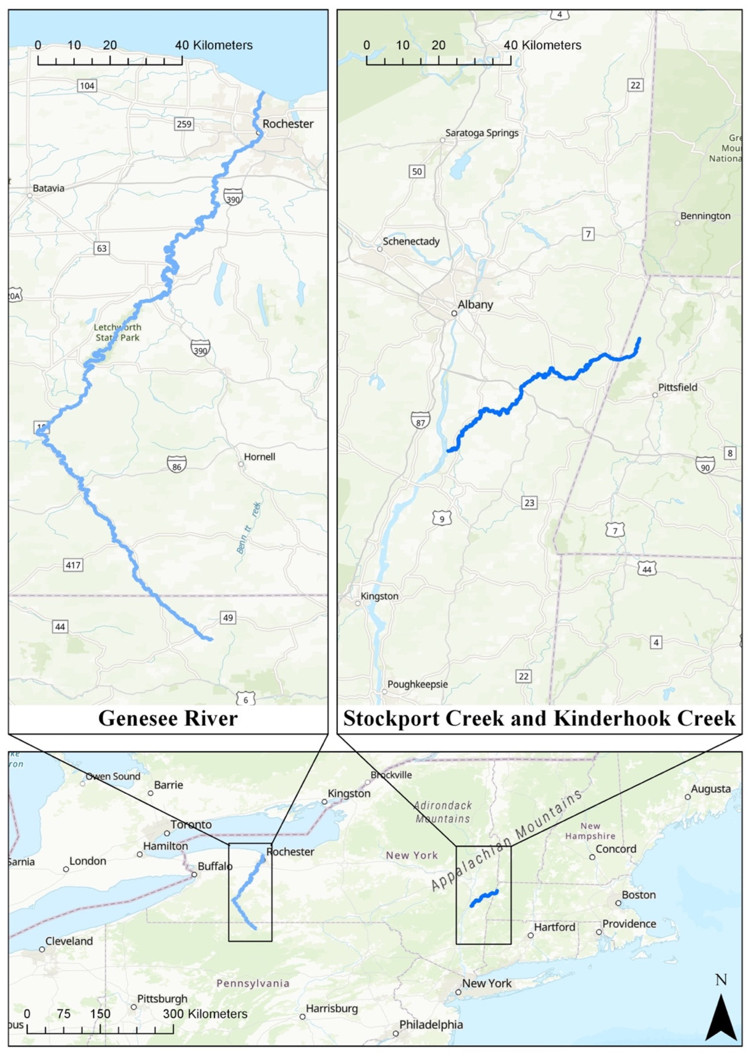
2.1. Site Description

This study focused on two watersheds in the north-eastern United States (US): the Genesee River watershed and the Hudson River watershed (Figure 1). The mainstem of the Genesee River served as a test site for methodology development, while we used the Stockport and Kinderhook Creek site in the Hudson River watershed for process validation. The combination of streams within the selected sites offered a comprehensive analysis including both small and large streams. Both sites are included in an active campaign by the New York State (NYS) Department of Environmental Conservation (DEC) to restore riparian vegetation to improve stream health and water quality [20].
The Genesee River flows north from Gold, Pennsylvania (elevation: 693 m) to enter Lake Ontario in Rochester, New York (elevation: 74.5 m). The river has a total length of 247 km and a 6408 km2 drainage area with land cover along the river corridor dominated by agriculture (52%) and forest (40%), with smaller amounts of developed land (5%), including a mixture of residential, commercial, and industrial uses, wetlands and water (2%), and other non-developed lands (1%) [21]. The New York Natural Heritage Program describes the Genesee River (Figure 1) as being in poor ecological health with high ecosystem stress [22]. We define the northern end of our study area using United States Geological Survey (USGS) stream gauge #04231600 in Rochester, NY, USA. The southern end was located at 41.939°N, 77.813°W following Makarewicz et al. [21].
Stockport Creek and its tributary Kinderhook Creek (Figure 1) are both located in the Stockport watershed, which is the second largest tributary watershed to the tidal Hudson River [23]. Kinderhook Creek flows from Hancock, Massachusetts (elevation: 376 m), south into Stockport Creek, which then enters the Hudson River mainstem in Stockport, New York (elevation: 0.1 m) with a total length of 83 km and a 1335 km2 drainage area. Land cover in the area is dominated by forest (71%), agriculture (21%) and other developed lands (8%) [23].

2.2. Data

This study used United States Department of Agriculture (USDA) National Agriculture Imagery Program (NAIP) imagery [24], which we accessed through Google Earth Engine [25]. The airborne orthorectified images in the NAIP collection are acquired at 1 m ground sampling distance during the growing season. The combination of high spatial, moderate spectral, and low temporal resolution in the NAIP dataset makes it well suited for periodic interpolation of detailed information on the boundaries of river channels and identification of riparian vegetation. This study used four-band (blue, green, red, and near infrared) 2015 NAIP imagery. Three auxiliary datasets were used to assist in delineation and assessing uncertainty: (1) USGS National Hydrography Dataset (NHD) [26]; (2) United States Census Bureau Places and Urban Area dataset [27]; and (3) NYS Park boundaries [28].

2.3. Delineation Processes

We sought to address the lack of published studies [5] that map both river channels and riparian vegetation at high spatial resolution (1 m or higher) over large extents. We used Google Earth Engine to efficiently classify riparian vegetation [25] and integrated geospatial data (e.g., NHD) to improve delineation accuracy. Boothroyd et al. [29] has demonstrated an increasing interest in using Google Earth Engine for large-scale fluvial geomorphology applications such as mapping river channels over large areas. Our approach adapted the satellite-based method of Monegaglia et al. [30] to semi-automatically map river channel boundaries using NAIP aerial photography and generate a map of riparian vegetation. We delineated channel boundaries and then performed a binary land cover classification to identify vegetation within the delineated riparian zones. Details of these two major steps are described below.

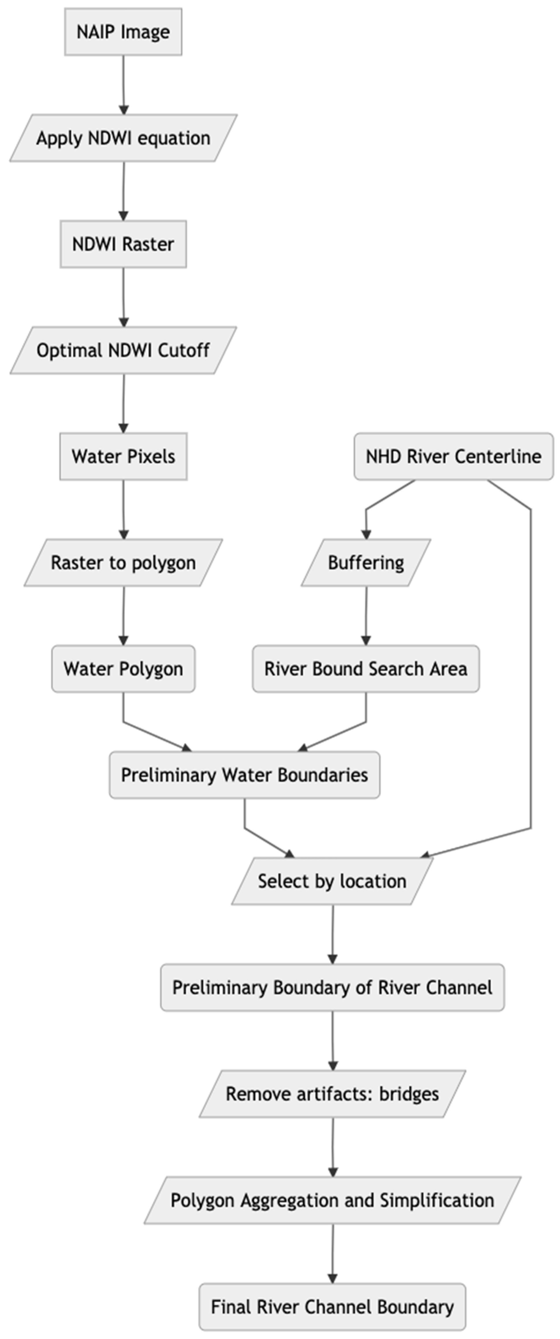
2.3.1. Step 1: Channel Boundary and Riparian Zone Delineation

We used a semi-automated approach to delineate river channel boundaries by integrating information extracted from the NAIP images with NHD centerline data (Figure 2). The method began by constructing a multi-band Normalized Difference Water Index (NDWI) from the selected NAIP image. The NDWI (Equation (1)) combines green and near-infrared (NIR) reflectance and is frequently utilized for extracting surface water features [31].
N D W I = G r e e n N I R G r e e n + N I R
McFeeters [32] found NDWI values of 0.3 generated from QuickBird imagery were an ideal cut-off for extracting water features in various regions. Based on this starting point, we tested values from 0–0.6 and through visual analysis found 0.4 was best for extracting surface water features in our study. We generated an NDWI mask using the selected cut-off for surface water extraction and converted this to a polygon vector layer that contained all of the potential surface water features. To improve computational efficiency, we applied a 200 m buffer along each side of the NHD river centerlines to limit the channel boundary search area. Selection of the 200 m buffer size was based on empirical testing to guarantee inclusion of the entire river channel and consideration of possible uncertainties in NHD data. We selected preliminary channel boundary polygons based on the intersection of the NDWI vector layer and the NHD buffer. We then manually removed non-river artifacts, such as road and railroad bridges, and smoothed the river channel boundary. We utilized a manual approach in this study due to the small number of artifacts presented in the image (n = 16). For a larger study area, or a region with a more complex built environment, we would recommend exploring automation. For example, publicly available road centreline data, e.g., US Census Topologically Integrated Geographic Encoding and Referencing (TIGER) products could be used to identify potential bridge locations. However, manual verification is likely still needed to confirm bridge removal accuracy.
The riparian zone in this study was defined as the region within 90 m of the river channel boundary. Sweeney and Newbold [33] and Hill [34] both suggested 90 m buffers as optimal to achieve the highest possible sediment and nutrient removal efficiency, which is relevant for pollution mitigation within our selected rivers. Multiple variable-width riparian zone delineation processes have been proposed [19,35]. However, these methods rely heavily on accurate and high spatial resolution DEMs, and such products are not widely available at 1 m spatial resolution. Thus, we used fixed width delineation for this study.

2.3.2. Step 2: Classifying Vegetation vs. Non-Vegetation within the Riparian Zone

We performed a binary classification in Google Earth Engine to identify vegetation within the riparian zone. The vegetation class included forests and shrubland, while the non-vegetation class included agricultural fields, roads, buildings, parking lots, and grassland. The classification process applied a random forest classifier to the NAIP imagery using Google Earth Engine [29]. Classification inputs included the four NAIP image bands and a normalized difference vegetation index (NDVI, (Equation (2))) derived from the red and NIR bands.
N D V I = R e d N I R R e d + N I R
Based on prior experimentation, we used 200 trees, set variables per split to 1, minimum leaf population to 1, and bag fraction to 0.5; further details of the classification process are available in Pu et al. [5]. We used aerial images because they have been applied for riparian vegetation delineation since the 1930s and provide high quality riparian vegetation coverage information [36]. With excellent spatial resolution, repeated temporal sampling, and no access cost, NAIP images are a prime candidate to analyse riparian vegetation coverage in the United States. The random forest classifier [37] was selected based on prior riparian vegetation delineation research by Hayes et al. [38] that successfully utilized this classifier for NAIP images. The riparian vegetation classification used 900 randomly sampled reference pixels manually labelled as either vegetation or non-vegetation class through photo interpretation of the NAIP image. The photo interpretation class was assigned through agreement of two trained photo-interpreters. Additionally, we used field observations and Google Earth Street images to validate manual interpretations for approximately half of the reference pixels. The output of the random forest classifier provided a preliminary riparian vegetation layer. As a second processing step, we located and removed all agricultural vegetation. Agricultural fields are a large source of nonpoint source pollution in the study area and are the largest source of phosphorus in the Genesee River [39]. Thus, we excluded agricultural vegetation because it does not provide key benefits such as filtering pollutants and trapping sediments. We used a combination of the multi-band NDVI) and NIR band texture (local Geary’s C, (Equation (3))) to remove agricultural vegetation.
C i = j w i j   ( z i z j ) 2
where zi is the NIR response at location i, zj is the NIR response at location j, wij are the elements of the spatial weights matrix computed as the distance between i and j. Selection of threshold values for NDVI and local Geary’s C were based on trial-and-error testing using randomly selected pixels across the study area. We ultimately utilized NDVI > 0 and local Geary’s C > 200 to separate agricultural and non-agricultural vegetation.

2.4. Analysis Design

2.4.1. Accuracy Assessment

We established a framework to assess riparian vegetation delineation accuracy by considering accuracy of both channel boundary delineation and riparian vegetation classification. We used conventional confusion matrices [40] for pixel-based accuracy assessment of channel boundary delineation (water vs. non-water) and riparian vegetation classification (vegetation vs. non-vegetation). Pixel-based accuracy was expressed in terms of overall accuracy (OA) as well as class producer’s accuracy (PA) and user’s accuracy (UA). An object-based approach [41] was also used to assess the difference between manually delineated reference channels and those generated by the automated delineation procedure. Object-based accuracy was expressed in terms of distance between the automatically and manually delineated channel boundaries.
Channel boundary delineation pixel-based accuracy considered the PA and UA for the water class. Overall accuracy and the non-water class statistics are heavily impacted by the area of the search zone; that is, extending the analysis areas will increase the amount of non-water areas, thus likely artificially increasing overall and non-water delineation accuracy. Since class-based accuracy statistics (UA and PA) for the water class do not change with area variations of the search zone, we focused on these statistics generated from within 200 m of the NHD river centreline. The 200 m zone was selected because it captured the maximum stream width across the study areas. Reference river channel was derived at a scale of 1:1000 with heads up digitizing of the NAIP images in ArcMap.
A second measure of delineation accuracy of the channel boundary used an object-based approach. According to Radoux and Bogaert [41] and Kucharczyk et al. [42], there is no standard approach to assess or estimate errors in object delineation. Positional accuracy can be expressed using point-based measures, e.g., root mean square error [17], or through surface-based methods [43]. Surface-based methods treat a delineated polygon of interest as an entity that is compared against a reference polygon. We selected an approach that has previously been utilized to estimate boundary error [42,43,44]. We calculated the proportion of the mapped channel area within variable-size buffers established around a manually delineated reference channel. The buffer distance started at 1 m, and 5 m, and then extended to 30 m in 5 m intervals. We then estimated the size of the buffer needed to encompass 50% of the mapped channel area and report this object-based channel boundary offset distance (D50).
Accuracy of the riparian vegetation classification was quantified using 5000 visually interpreted pixels selected by simple random sampling within the 90 m riparian zone. Reference pixels were derived at a scale of 1:1000 with heads up digitizing of the NAIP images in ArcMap. Labelling of vegetation and non-vegetation pixels used the NAIP image bands and derived vegetation indices in conjunction with auxiliary datasets, which included United States Census Bureau Places and Urban Area dataset for identifying potential non-vegetation pixels, and New York State Park boundaries for verifying vegetated pixels. An independent photo interpreter who had no role in producing the map products obtained the reference datasets used to perform the validation. Accuracy metrics and accompanying standard errors were estimated using equations from Olofsson [45].

2.4.2. Factors Impacting Accuracy

We also considered potential causes of inaccuracy in both channel boundary delineation and riparian vegetation classification to guide future efforts to improve accuracy of riparian vegetation delineation. We explored two factors for channel boundary delineation (stream order and shadows) and three factors for riparian vegetation classification (land use, width of the riparian zone, and shadows). Stream order measures the placement of a stream within the tributary hierarchy [46]. We considered this factor because higher stream orders generally have greater stream width, which is expected to increase channel boundary detection accuracy [47]. Several approaches for labelling stream order have been proposed, with the method developed by Strahler [48] still popular. We determined stream order using the RivEX tool, which was originally developed by Gleyzer et al. [49] using Strahler’s stream ordering method. We used this ArcMap-based plugin to segment the rivers in the two study areas by labelling stream order based on the given NHD stream centerline. We generated confusion matrices to assess the impact of stream order on accuracy.
Land use was evaluated to determine if variations in riparian vegetation coverage associated with different land use patterns impact vegetation classification accuracy. Such a hypothesis was supported by a previous study by Hollenhorst et al. [16]. Within the 90 m fixed width riparian zone, we manually identified land use in the NAIP imagery using three classes: developed, natural, and agriculture. Census data supported delineating areas of developed land use, while NYS park boundaries assisted in mapping natural land use. We generated confusion matrices to access the impact of land use on accuracy.
Width of riparian zone was evaluated as another influential factor that may impact riparian vegetation classification accuracy. Hollenhorst et al. [16] reported that larger riparian zone width led to higher overall accuracy, which we explored in this study. We used three buffer sizes (30 m, 60 m and 90 m), and selected sample pixels within each buffer size to generate confusion matrices to determine the impact of fixed riparian zone width on vegetation classification accuracy.
Shadows have long been reported to impact mapping accuracy in various applications [18], and we explored whether they may influence both channel boundary delineation and riparian vegetation classification accuracy. We considered shadows caused by changing illumination due to objects (e.g., trees or buildings) and topography (e.g., hills or valleys). We identified areas of shadows using the modified C 3 * (Equation (4)) index method developed by Besheer and Abdelhafiz [50].
C 3 * = a r c t a n ( B l u e m a x ( G r e e n ,   R e d ,   N I R ) )
Their method identifies shadowed regions based on the inflection point in the histogram of C 3 * values after masking water regions and yielded above 94% accuracy in areas with various land cover compositions. We determined where the manually delineated channel fell within shadowed regions and generated confusion matrices separately for shaded and illuminated areas to consider the impact of image shadows on both channel boundary and riparian vegetation delineation accuracy. We did not need to apply a water mask because we focused exclusively on the previously identified riparian zone.

3. Results

We delineated channel boundaries and classified riparian vegetation at the Genesee River and Stockport and Kinderhook Creek sites (Table 1), detecting channel boundaries up to 5th order streams for both study sites. Figure 3 and Figure 4 show examples of delineated channel boundary and classified riparian vegetation, respectively. Coverage of shadow within the fixed (90 m) width riparian zone was 5% at Genesee River and 20% at Stockport and Kinderhook Creek. Computational processing time at Genesee River was 31 min for channel boundary delineation and 3 min for riparian vegetation classification; Stockport and Kinderhook Creek processing times were 12 min (channel boundary delineation) and 1 min (riparian vegetation classification). The majority of personnel time (8 days for Genesee River and 5 days for Stockport and Kinderhook Creek) was spent in generating reference data through manual delineation of channel boundaries and manual classification of vegetation vs. non-vegetation pixels. Manual post processing to enhance the automatic delineation of channel boundaries (e.g., removing bridge crossings) took an additional day.

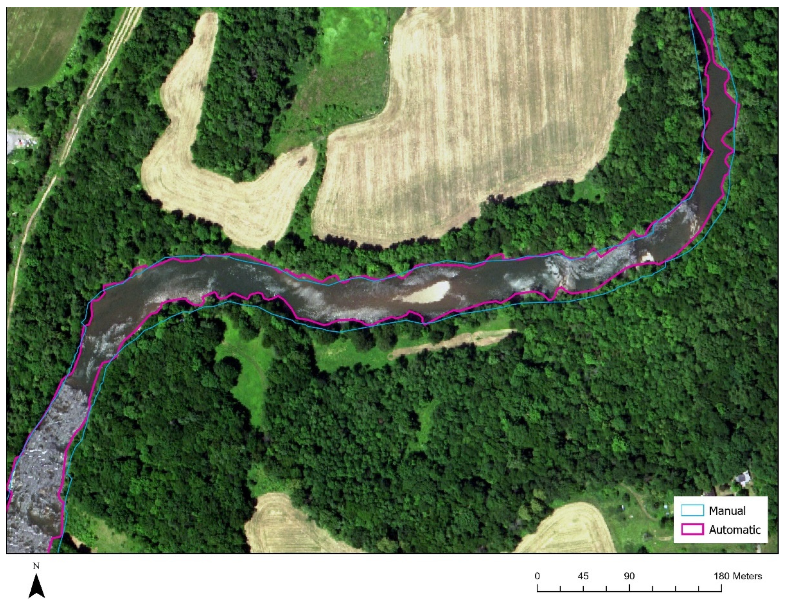
3.1. Channel Boundary Delineation Accuracy

UA and PA for the water class in the channel boundary delineation were generally above 80% for both sites, with UA for shadowed regions in the smallest channels (5th order) being the only exception (Table 2). The object-based accuracy assessment revealed that the buffer distance from the reference channel that contained at least 50% of the delineated channel area was generally less than 5 m. Larger streams (i.e., higher stream order) had higher UA, and generally higher PA, though the highest PA at the Genesee River site was for the 6th order streams. Presence of shadow had a minor (less than 3%) influence on both PA and UA. The object-based channel boundary offset distance decreased up to 3 m when shadowed areas were removed from the analysis.

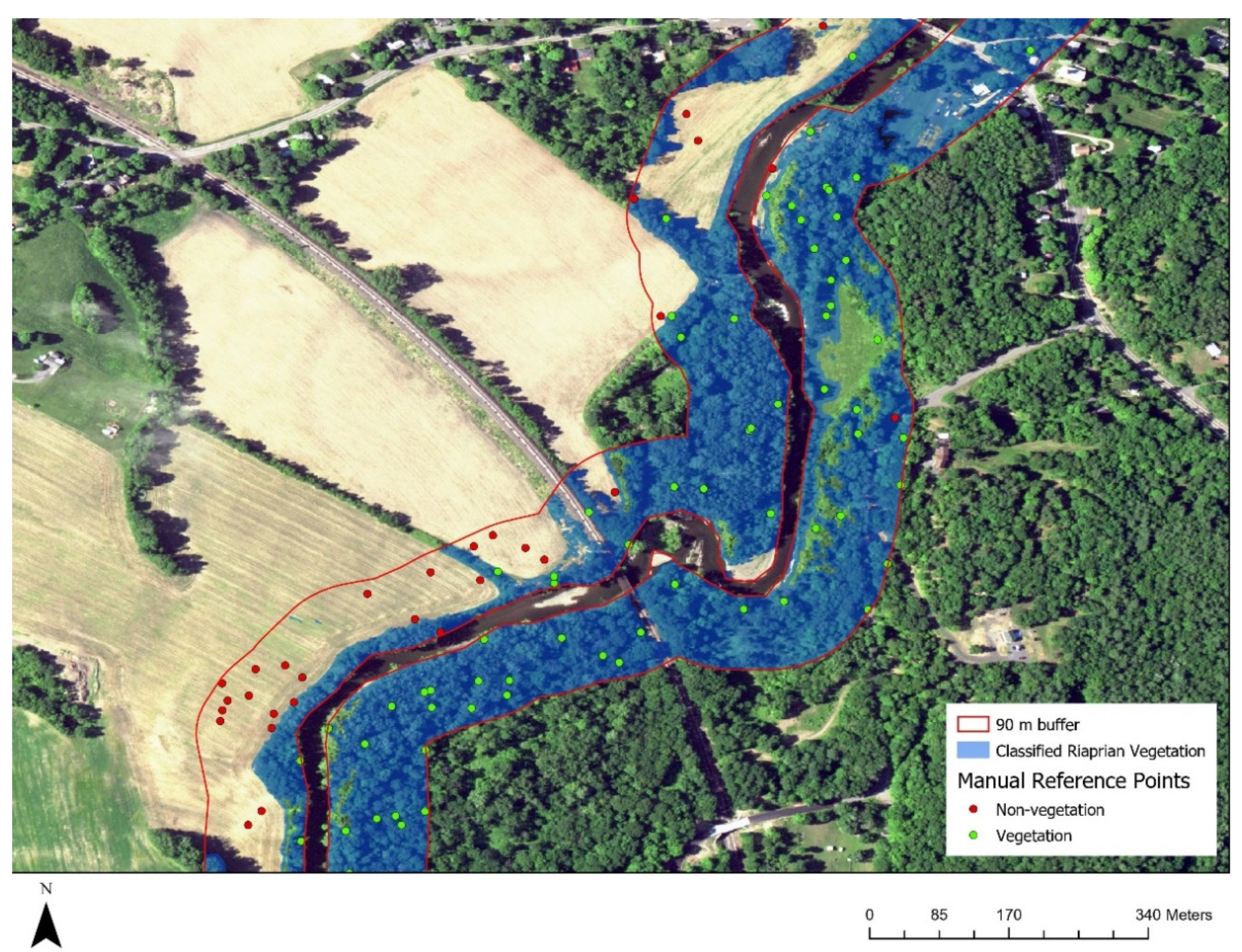
3.2. Riparian Vegetation Classification Accuracy

Overall accuracy of the vegetation vs. non-vegetation classification within the 90 m riparian zone was 87% for the Genesee River (Table 3) and 96% for the Stockport and Kinderhook Creek (Table 4) sites. UA was higher for the vegetation class (96–98%) than non-vegetation (75–86%), while the reverse was true for PA (80–97% and 90–96% for vegetation and non-vegetation, respectively). Table 3 and Table 4 also summarizes the classification accuracy for three different land use types (agriculture, developed, and natural) and for three riparian zone widths (30 m, 60 m, and 90 m). Developed land use had the lowest OA (79–94%), while agricultural and natural land use OAs were higher (88–98%). Vegetation classification accuracy for the three riparian zone widths (30 m, 60 m, and 90 m) had small differences (average of 3%) in overall and class accuracies. In contrast with the channel delineation accuracy, removing regions with shadows from the riparian vegetation classification did not substantially change the overall classification accuracy at the Genesee River site, though there were larger differences in the class statistics, with shaded areas of vegetation tending to have lower UA and PA (Table 3). A larger proportion of the Stockport and Kinderhook Creek site was shaded but while overall accuracy at that site was lower in the shaded areas (91%) compared to the fully illuminated areas (97%), there was little difference compared to the OA for all regions (96%) (Table 4).

4. Discussion

4.1. Importance of Considering Channel Delineation Accuracy

To our knowledge, no prior study has reported both channel boundary delineation and vegetation classification accuracy when delineating riparian vegetation. However, our results show both components influence the quality of riparian vegetation delineation. We found that 50% of automatically delineated river channel polygons could be up to 5 m away from the corresponding reference channel polygon. In a fixed riparian zone framework, riparian buffers are generated directly from the delineated channel boundary, thus positional inaccuracy in the river channel propagates to inaccurate riparian buffer zones and ultimately produces inaccurate maps documenting the location and coverage of riparian vegetation. Positional accuracy of riparian vegetation is a critical requirement for aiding field-based riparian management and restoration efforts [51]. Inclusion of channel boundary accuracy is especially important in the fixed width riparian zone framework. In a variable width riparian zone framework, accuracy of channel boundary delineation may be replaced by DEM accuracy [19]. However, we still lack convenient and widespread access to high quality DEM. Quantification of the accuracy of these products is still under active development [52], and may not be applicable across broad scales. Thus, channel boundary accuracy from passive imagery still remains an issue of concern, especially given the higher cost required to acquire lidar-derived DEMs [53].
Accurately detecting channel boundaries is a critical concern for riparian vegetation studies. However, channel boundary mapping accuracy is also important for other studies that are related to channel margins, such as lateral channel migration studies [17]. Donovan et al. [17] and Lea and Legleiter [54] recently introduced new frameworks to assess uncertainty. However, both focused on specific issues, rather than developing broadly applicable techniques. Donovan et al. [17] assessed producer’s error in the manual delineation process, whereas Lea and Legleiter [54] addressed image registration, which is particularly relevant in change studies that utilize multiple images of a location [55]. While the accuracy of manual digitization is important, manual approaches have practical limitations and cannot be applied over large areas. Consequently, a broader focus on uncertainty for semi-automatic or automatic channel boundary mapping accuracy is needed, especially in the context of using Google Earth Engine [29]. Our approach addresses this issue by demonstrating a method to assess accuracy in semi-automatically or automatically mapped channel boundaries through applying a well-established map accuracy approach [56] in conjunction with an object-based accuracy assessment [41].

4.2. Factors Impacting Channel Boundary Delineation and Riparian Vegetation Classification Accuracy

4.2.1. Stream Order Impact

Stream order had moderate impact on channel boundary delineation accuracy. The larger river channels associated with the higher stream order increased the user’s accuracy and channel boundary delineation accuracy while decreasing producer’s accuracy (Table 2). The decrease in the user’s accuracy and boundary accuracy in the narrower channels could be associated with the greater influence of overhanging vegetation [17]. Future riparian vegetation delineation studies could focus greater effort on improving smaller stream order channel boundary delineation accuracy, which would offer an efficient way to improve the overall accuracy of the entire river channel boundary delineation. Such efforts may utilize recently published methods that incorporate lidar and deep learning models to improve channel boundary delineation accuracy in smaller streams [57].

4.2.2. Land Use and Riparian Width Impact

Land use impacted the vegetation vs. non-vegetation classification accuracy corroborating the results of Smith et al. [58] and Tran et al. [59]. Our results confirm prior studies that found regions with developed land use had lower OA than agricultural and natural areas, possibly due to the more complex nature of developed regions. Our results also confirm the findings of Hollenhorst et al. [16] regarding higher heterogeneity of land cover types decreasing riparian vegetation delineation accuracy. In contrast with Hollenhorst et al. [16]’s study, which used manual interpretation of aerial photos, we used a semi-automatic approach that increased the efficiency of riparian vegetation classification.

4.2.3. Image Shadow Effects

Shadows in imagery have long been reported to impact accuracy in mapping applications [18]. Our study found that image shadows did influence channel boundary delineation, with the channel more challenging to define accurately in shaded regions. There were also impacts on riparian vegetation classification with overall accuracy between shaded and fully illuminated regions varying by as much as 5%. However, this did not have a practical influence on classification accuracy. The Genesee River site had only a 2% coverage of shaded pixels and including these shaded regions did not negatively impact overall accuracy of the classification. With 20% coverage of shadow at the Stockport and Kinderhook site, inclusion of shaded areas still only led to a small (1%) decrease in overall map accuracy. The reduced classification accuracy in shaded regions may be a more significant issue in areas where the extent of shadow in an image is greater.

4.2.4. Future Work

Abood et al. [35], Holmes and Goebel [19], and Salo and Theobald [10] applied variable width riparian zone definitions and methods to delineate riparian zone vegetation. Variable width riparian zone mapping processes typically rely on high spatial resolution DEMs for delineation of riparian zones. Such reliance limits wider adoption of these approaches due to restricted availability—both spatially and temporally—of DEMs with pixel size ≤ 1 m. Due to these limitations, there is a continued need for fixed width riparian zone delineation methods to support analysis across various scales. As high spatial resolution DEMs become more widely available, assessment of the quality of variable width riparian zone mapping approaches will need to address the accuracy of the DEM used. Future work should compare riparian vegetation delineation accuracies using various riparian zone definitions.
The channel boundary delineation and accuracy quantification methods developed in this article can be applied to other fields of study that rely on accurate channel boundary data, such as the study of planform channel migration rates. Current methods to delineate river channels based on remotely sensed data are still very much reliant on manual mapping approaches [54,60]. There are some automatic channel delineation approaches, but many of these rely on methods that are not readily available, or do not incorporate rigorous map accuracy quantification [17]. The approach applied in this study improves upon prior methods in terms of semi-automatically delineating and assessing channel boundary accuracy.

5. Conclusions

This study used a semi-automatic approach to delineate river channel boundaries and classify riparian vegetation using a freely available public dataset (NAIP) and cloud-based technology (Google Earth Engine). The subsequent evaluation holistically quantified the accuracy of riparian vegetation delineation by including assessment of both channel boundary and riparian classification accuracy and demonstrated that both elements are critical in terms of comprehensively understanding the quality of riparian vegetation maps. Through our analysis, we also considered factors that can impact channel boundary and riparian vegetation classification accuracy. We found stream order impacted channel boundary delineation accuracy while land use and riparian zone width both impacted the riparian vegetation classification accuracy. Shadowed regions created a greater challenge for channel delineation accuracy and could significantly impact riparian delineation processes, particularly in steep topography or if imagery is acquired at lower sun elevation angles leading to greater differential illumination.
Stakeholders need a straightforward means to delineate river channel boundaries and riparian vegetation extent while assessing accuracy of both components to effectively use remotely sensed data to map riparian vegetation. The procedures established in this study highlight factors that influence the quality of riparian characterization and provide a means to conduct riparian vegetation mapping and accuracy assessment that can be applied across other regions and using other datasets.

Supplementary Materials

The following are available online at https://www.mdpi.com/article/10.3390/rs13224645/s1.

Author Contributions

Conceptualization, G.P.; methodology, G.P., L.J.Q. and S.V.S.; data curation, G.P.; formal analysis, G.P.; funding acquisition, G.P. and L.J.Q.; writing—original draft, G.P.; project administration, L.J.Q.; supervision, L.J.Q.; writing—review and editing, L.J.Q. and S.V.S. All authors have read and agreed to the published version of the manuscript.

Funding

This work was supported by the U.S. Geological Survey Grant/Cooperative Agreement (G18AP00077) and The New York State Water Resources Institute.

Institutional Review Board Statement

Not applicable.

Informed Consent Statement

Not applicable.

Data Availability Statement

The data that support the findings of this study are openly available in figshare at https://doi.org/10.6084/m9.figshare.15086640, Last accessed 16 November 2021.

Acknowledgments

We thank colleagues at SUNY ESF for providing constructive and helpful comments on early drafts of this manuscript. We gratefully acknowledge constructive remarks by editors and anonymous reviewers.

Conflicts of Interest

The authors declare no conflict of interest.

References

  1. Baker, M.E.; Weller, D.E.; Jordan, T.E. Improved methods for quantifying potential nutrient interception by riparian buffers. Landsc. Ecol. 2006, 21, 1327–1345. [Google Scholar] [CrossRef]
  2. Iverson, L.R.; Szafoni, D.L.; Baum, S.E.; Cook, E.A. A Riparian Wildlife Habitat Evaluation Scheme Developed Using GIS. Environ. Manag. 2001, 28, 639–654. [Google Scholar] [CrossRef]
  3. Singh, R.; Tiwari, A.K.; Singh, G.S. Managing riparian zones for river health improvement: An integrated approach. Landsc. Ecol. Eng. 2021, 17, 195–223. [Google Scholar] [CrossRef]
  4. Klemas, V. Remote Sensing of Riparian and Wetland Buffers: An Overview. J. Coast. Res. 2014, 297, 869–880. [Google Scholar] [CrossRef] [Green Version]
  5. Pu, G.; Quackenbush, L.J.; Stehman, S.V. Using Google Earth Engine to Assess Temporal and Spatial Changes in River Geomorphology and Riparian Vegetation. JAWRA J. Am. Water Resour. Assoc. 2021, 57, 789–806. [Google Scholar] [CrossRef]
  6. Piégay, H.; Arnaud, F.; Belletti, B.; Bertrand, M.; Bizzi, S.; Carbonneau, P.; Dufour, S.; Liébault, F.; Ruiz-Villanueva, V.; Slater, L. Remotely sensed rivers in the Anthropocene: State of the art and prospects. Earth Surf. Process. Landforms 2020, 45, 157–188. [Google Scholar] [CrossRef]
  7. Claggett, P.R.; Okay, J.A.; Stehman, S.V. Monitoring Regional Riparian Forest Cover Change Using Stratified Sampling and Multiresolution Imagery. JAWRA J. Am. Water Resour. Assoc. 2010, 46, 334–343. [Google Scholar] [CrossRef]
  8. Fu, B.; Burgher, I. Riparian vegetation NDVI dynamics and its relationship with climate, surface water and groundwater. J. Arid. Environ. 2015, 113, 59–68. [Google Scholar] [CrossRef]
  9. Yang, X. Integrated use of remote sensing and geographic information systems in riparian vegetation delineation and mapping. Int. J. Remote Sens. 2007, 28, 353–370. [Google Scholar] [CrossRef]
  10. Salo, J.A.; Theobald, D.M. A Multi-scale, Hierarchical Model to Map Riparian Zones. River Res. Appl. 2016, 32, 1709–1720. [Google Scholar] [CrossRef]
  11. Ali, S.S.; Corner, R. Land cover change detection using ASTER and Landsat-7 ETM+ images: An application to forest resource management. In Proceedings of the 2003 Spatial Sciences Conference, Canberra, Australia, 22–26 September 2003; pp. 22–26. [Google Scholar]
  12. Johansen, K.; Phinn, S.; Witte, C. Mapping of riparian zone attributes using discrete return LiDAR, QuickBird and SPOT-5 imagery: Assessing accuracy and costs. Remote Sens. Environ. 2010, 114, 2679–2691. [Google Scholar] [CrossRef]
  13. Wasser, L.; Chasmer, L.; Day, R.; Taylor, A. Quantifying land use effects on forested riparian buffer vegetation structure using LiDAR data. Ecosphere 2015, 6, art10. [Google Scholar] [CrossRef]
  14. Dunford, R.; Michel, K.; Gagnage, M.; Piégay, H.; Trémelo, M.-L. Potential and constraints of Unmanned Aerial Vehicle technology for the characterization of Mediterranean riparian forest. Int. J. Remote Sens. 2009, 30, 4915–4935. [Google Scholar] [CrossRef]
  15. Räpple, B.; Piégay, H.; Stella, J.C.; Mercier, D. What drives riparian vegetation encroachment in braided river channels at patch to reach scales? Insights from annual airborne surveys (Drôme River, SE France, 2005–2011). Ecohydrology 2017, 10, e1886. [Google Scholar] [CrossRef]
  16. Hollenhorst, T.P.; Host, G.E.; Johnson, L.B. Scaling Issues in Mapping Riparian Zones with Remote Sensing Data: Quantifying Errors and Sources of Uncertainty. In Scaling and Uncertainty Analysis in Ecology; Springer: Dordrecht, The Netherlands, 2006; pp. 275–295. [Google Scholar] [CrossRef]
  17. Donovan, M.; Belmont, P.; Notebaert, B.; Coombs, T.; Larson, P.; Souffront, M. Accounting for uncertainty in remotely-sensed measurements of river planform change. Earth-Sci. Rev. 2019, 193, 220–236. [Google Scholar] [CrossRef]
  18. Finlayson, G.D.; Hordley, S.D.; Lu, C.; Drew, M.S. On the removal of shadows from images. IEEE Trans. Pattern Anal. Mach. Intell. 2006, 28, 59–68. [Google Scholar] [CrossRef] [PubMed]
  19. Holmes, K.L.; Goebel, P.C. A functional approach to riparian area delineation using geospatial methods. J. For. 2011, 109, 233–241. [Google Scholar] [CrossRef]
  20. NYS DEC. Trees for Tribs. Available online: www.dec.ny.gov/animals/77710.html (accessed on 16 November 2021).
  21. Makarewicz, J.C.; Lewis, T.W.; Rea, E.; Winslow, M.J.; Pettenski, D. Using SWAT to determine reference nutrient conditions for small and large streams. J. Great Lakes Res. 2015, 41, 123–135. [Google Scholar] [CrossRef]
  22. Conley, A.K.; Howard, T.G.; White, E.L. Great Lakes Basin Riparian Opportunity Assessment; New York Natural Heritage Program, State University of New York College of Environmental Science and Forestry: Albany, NY, USA, 2016; Available online: https://www.nynhp.org/projects/great-lakes-riparian-assessment/ (accessed on 16 November 2021).
  23. Martino, F. Description and Inventory of the Stockport Creek Watershed. 2012. Available online: http://www.stockportwatershed.org/docs/Stockport_Watershed_Description_and_Inventory.pdf (accessed on 16 November 2021).
  24. USDA-FSA-APFO Aerial Photography Field Office National Geospatial Data Asset (NGDA) NAIP Imagery. 2016. Available online: https://www.fsa.usda.gov/programs-and-services/aerial-photography/imagery-programs/naip-imagery/ (accessed on 16 November 2021).
  25. Gorelick, N.; Hancher, M.; Dixon, M.; Ilyushchenko, S.; Thau, D.; Moore, R. Google Earth Engine: Planetary-scale geospatial analysis for everyone. Remote Sens. Environ. 2017, 202, 18–27. [Google Scholar] [CrossRef]
  26. United States Geological Survey National Hydrography Dataset. Available online: https://viewer.nationalmap.gov/basic/?basemap=b1&category=nhd&title=NHDView (accessed on 16 November 2021).
  27. United States Census Bureau Places and Urban Area Dataset. Available online: https://www.census.gov/geographies/mapping-files/time-series/geo/carto-boundary-file.2015.html (accessed on 16 November 2021).
  28. New York State Parks Recreation & Historic Preservation New York State Historic Sites and Park Boundary. Available online: https://gis.ny.gov/gisdata/inventories/details.cfm?DSID=430 (accessed on 16 November 2021).
  29. Boothroyd, R.J.; Williams, R.D.; Hoey, T.B.; Barrett, B.; Prasojo, O.A. Applications of Google Earth Engine in fluvial geomorphology for detecting river channel change. Wiley Interdiscip. Rev. Water 2021, 8, e21496. [Google Scholar] [CrossRef]
  30. Monegaglia, F.; Zolezzi, G.; Güneralp, I.; Henshaw, A.J.; Tubino, M. Automated extraction of meandering river morphodynamics from multitemporal remotely sensed data. Environ. Model. Softw. 2018, 105, 171–186. [Google Scholar] [CrossRef]
  31. McFeeters, S.K. The use of the Normalized Difference Water Index (NDWI) in the delineation of open water features. Int. J. Remote Sens. 1996, 17, 1425–1432. [Google Scholar] [CrossRef]
  32. McFeeters, S.K. Using the Normalized Difference Water Index (NDWI) within a Geographic Information System to Detect Swimming Pools for Mosquito Abatement: A Practical Approach. Remote Sens. 2013, 5, 3544–3561. [Google Scholar] [CrossRef] [Green Version]
  33. Sweeney, B.W.; Newbold, J.D. Streamside Forest Buffer Width Needed to Protect Stream Water Quality, Habitat, and Organisms: A Literature Review. JAWRA J. Am. Water Resour. Assoc. 2013, 50, 560–584. [Google Scholar] [CrossRef]
  34. Hill, A.R. Landscape Hydrogeology and its Influence on Patterns of Groundwater Flux and Nitrate Removal Efficiency in Riparian Buffers. JAWRA J. Am. Water Resour. Assoc. 2017, 54, 240–254. [Google Scholar] [CrossRef]
  35. Abood, S.A.; MacLean, A.L.; Mason, L. Modeling Riparian Zones Utilizing DEMS and Flood Height Data. Photogramm. Eng. Remote Sens. 2012, 78, 259–269. [Google Scholar] [CrossRef]
  36. Dufour, S.; Muller, E.; Straatsma, M.; Corgne, S. Image Utilisation for the Study and Management of Riparian Vegetation: Overview and Applications. In Fluvial Remote Sensing for Science and Management; Carbonneau, R.E., Piégay, H., Eds.; Wiley: Hoboken, NJ, USA, 2012; pp. 215–239. [Google Scholar]
  37. Pal, M. Random forest classifier for remote sensing classification. Int. J. Remote Sens. 2005, 26, 217–222. [Google Scholar] [CrossRef]
  38. Hayes, M.M.; Miller, S.N.; Murphy, M. High-resolution landcover classification using Random Forest. Remote Sens. Lett. 2014, 5, 112–121. [Google Scholar] [CrossRef]
  39. NYS DEC. Hudson River Estuary Action Agenda 2015–2020. Available online: https://hudsonwatershed.org/wp-content/uploads/HREP-AA-2015.pdf (accessed on 16 November 2021).
  40. Story, M.; Congalton, R.G. Remote Sensing Brief Accuracy Assessment: A User’s Perspective. Photogramm. Eng. Remote Sens. 1986, 52, 397–399. [Google Scholar]
  41. Radoux, J.; Bogaert, P. Good Practices for Object-Based Accuracy Assessment. Remote Sens. 2017, 9, 646. [Google Scholar] [CrossRef] [Green Version]
  42. Kucharczyk, M.; Hay, G.; Ghaffarian, S.; Hugenholtz, C. Geographic Object-Based Image Analysis: A Primer and Future Directions. Remote Sens. 2020, 12, 2012. [Google Scholar] [CrossRef]
  43. Schöpfer, E.; Lang, S.; Albrecht, F. Object-fate analysis: Spatial relationships for the assessment of object transition and correspondence. In Lecture Notes in Geoinformation and Cartography; Springer: Berlin/Heidelberg, Germany, 2008; pp. 785–801. [Google Scholar] [CrossRef]
  44. Tatem, A.; Noor, A.; Hay, S. Assessing the accuracy of satellite derived global and national urban maps in Kenya. Remote Sens. Environ. 2005, 96, 87–97. [Google Scholar] [CrossRef] [Green Version]
  45. Olofsson, P.; Foody, G.M.; Herold, M.; Stehman, S.V.; Woodcock, C.E.; Wulder, M.A. Good practices for estimating area and assessing accuracy of land change. Remote Sens. Environ. 2014, 148, 42–57. [Google Scholar] [CrossRef]
  46. Leopold, L.B.; Wolman, M.G.; Miller, J.P. Fluvial Processes in Geomorphology; Dover Books on Earth Sciences; Dover Publications: New York, NY, USA, 1995; ISBN 9780486685885. [Google Scholar]
  47. Downing, J.A.; Cole, J.J.; Duarte, C.M.; Middelburg, J.; Melack, J.M.; Prairie, Y.; Kortelainen, P.; Striegl, R.G.; McDowell, W.; Tranvik, L.J. Global abundance and size distribution of streams and rivers. Inland Waters 2012, 2, 229–236. [Google Scholar] [CrossRef]
  48. Strahler, A.N. Quantitative analysis of watershed geomorphology. Trans. Am. Geophys. Union 1957, 38, 913–920. [Google Scholar] [CrossRef] [Green Version]
  49. Gleyzer, A.; Denisyuk, M.; Rimmer, A.; Salingar, Y. A Fast Recursive Gis Algorithm for Computing Strahler Stream Order in Braided Aand Nonbraided Networks. JAWRA J. Am. Water Resour. Assoc. 2004, 40, 937–946. [Google Scholar] [CrossRef]
  50. Besheer, M.; Abdelhafiz, A. Modified invariant colour model for shadow detection. Int. J. Remote Sens. 2015, 36, 6214–6223. [Google Scholar] [CrossRef]
  51. Gergel, S.E.; Stange, Y.; Coops, N.C.; Johansen, K.; Kirby, K.R. What is the Value of a Good Map? An Example Using High Spatial Resolution Imagery to Aid Riparian Restoration. Ecosystems 2007, 10, 688–702. [Google Scholar] [CrossRef]
  52. Lohani, B.; Ghosh, S.; Dashora, A. A review of standards for airborne LiDAR data acquisition, processing, QA/QC, and delivery. In Geospatial Infrastructure, Applications and Technologies: India Case Studies; Springer: Singapore, 2018; pp. 305–312. ISBN 9789811323300. [Google Scholar]
  53. Huylenbroeck, L.; Laslier, M.; Dufour, S.; Georges, B.; Lejeune, P.; Michez, A. Using remote sensing to characterize riparian vegetation: A review of available tools and perspectives for managers. J. Environ. Manag. 2020, 267, 110652. [Google Scholar] [CrossRef]
  54. Lea, D.M.; Legleiter, C.J. Refining measurements of lateral channel movement from image time series by quantifying spatial variations in registration error. Geomorphology 2016, 258, 11–20. [Google Scholar] [CrossRef]
  55. Leonard, C.M.; Legleiter, C.J.; Lea, D.M.; Schmidt, J.C. Measuring channel planform change from image time series: A generalizable, spatially distributed, probabilistic method for quantifying uncertainty. Earth Surf. Process. Landf. 2020, 45, 2727–2744. [Google Scholar] [CrossRef]
  56. Foody, G.M.; Atkinson, P.M. Uncertainty in Remote Sensing and GIS; Wiley: Chichester, UK, 2002; pp. 287–302. [Google Scholar] [CrossRef]
  57. Xu, Z.; Wang, S.; Stanislawski, L.V.; Jiang, Z.; Jaroenchai, N.; Sainju, A.M.; Shavers, E.; Usery, E.L.; Chen, L.; Li, Z.; et al. An attention U-Net model for detection of fine-scale hydrologic streamlines. Environ. Model. Softw. 2021, 140, 104992. [Google Scholar] [CrossRef]
  58. Tsintikidis, D.; Georgakakos, K.P.; Sperfslage, J.A.; Smith, D.E.; Carpenter, T.M. Precipitation Uncertainty and Raingauge Network Design within Folsom Lake Watershed. J. Hydrol. Eng. 2002, 7, 175–184. [Google Scholar] [CrossRef]
  59. Tran, T.V.; Julian, J.P.; De Beurs, K.M. Land Cover Heterogeneity Effects on Sub-Pixel and Per-Pixel Classifications. ISPRS Int. J. Geo-Inf. 2014, 3, 540–553. [Google Scholar] [CrossRef] [Green Version]
  60. Allen, D.C.; Wynn-Thompson, T.M.; Kopp, D.A.; Cardinale, B.J. Riparian plant biodiversity reduces stream channel migration rates in three rivers in Michigan, U.S.A. Ecohydrology 2018, 11, e1972. [Google Scholar] [CrossRef]
Figure 1. Map of studied streams in western (Genesee River) and eastern (Stockport and Kinderhook Creeks) New York State, US. Basemap is World Topographic Map.
Remotesensing 13 04645 g001
Figure 2. Flowchart of river channel delineation using NAIP images and NHD centerline data.
Remotesensing 13 04645 g002
Figure 3. Example results of manual vs. automatic delineated river channel boundary. Background image is 2015 NAIP. Center of map is located near Town of Stuyvesant Falls, New York State, United States.
Remotesensing 13 04645 g003
Figure 4. Example of classified riparian vegetation overlaid with manually classified reference points. Background image is 2015 NAIP. Center of map is located near Town of Chatham, New York State, United States.
Remotesensing 13 04645 g004
Table 1. Summary of area within the channel and covered by riparian vegetation for the Genesee River and Stockport and Kinderhook Creek sites.
StreamTotal Area within 90 m Riparian Zone (km2)Area within Channel Boundaries (km2)Area of Riparian Vegetation (km2)
Genesee River43.889.7122.51
Stockport and Kinderhook Creek12.861.9110.50
Table 2. Channel boundary delineation accuracy for Genesee River (GR) and Stockport and Kinderhook Creek (SKC) grouped by stream order and presence of image shadow. Expanded object-based accuracy assessment results are provided in the Supplementary Materials (Figures S1 and S2).
Stream OrderShadow PresentWater ClassObject Based
UA (%)PA (%)D50 (m)
GRSKCGRSKCGRSKC
5thYes768586813.53.1
No758587823.21.2
6thYes839691925.21.5
No829691953.00.3
7thYes95NA80NA3.5NA
No94NA83NA0.2NA
NA: Not applicable (no 7th order streams at SKC). D50: distance from reference channel to encompass 50% of mapped channel.
Table 3. Riparian vegetation classification accuracy of riparian zone along Genesee River characterized by land use and image shadow presence (full confusion matrices are provided in Table S1).
RZ Width (m)Land UseShadow/No ShadowOverall Map (%)Vegetation (%) Non-Vegetation (%)
OA (SE)UA (SE)PA (SE)UA (SE)PA (SE)
90All typesBoth 87 (1)96 (0)81 (1)76 (1)95 (1)
90AgricultureBoth 88 (1)96 (0)82 (1)79 (1)95 (1)
90DevelopedBoth79 (2)96 (1)67 (2)66 (3)96 (1)
90NaturalBoth88 (1)98 (1)85 (1)68 (3)95 (2)
90All typesNo Shadow only87 (1)97 (0)82 (1)74 (1)95 (1)
90All typesShadow only88 (2)67 (17)19 (6)89 (2)98 (1)
60All typesAll areas87 (1)97 (0)82 (1)75 (1)95 (1)
30All typesAll areas87 (1)97 (1)83 (1)74 (2)95 (1)
RZ: Riparian Zone, OA: Overall Accuracy, UA: User’s Accuracy, PA: Producer’s Accuracy and SE: Standard Error.
Table 4. Riparian vegetation classification accuracy riparian zone along Stockport and Kinderhook Creeks characterized by land use and image shadow presence (full confusion matrices are provided in Table S2).
RZ Width (m)Land UseShadow/No ShadowOverall Map (%)Vegetation (%) Non-Vegetation (%)
OA (SE)UA (SE)PA (SE)UA (SE)PA (SE)
90All typesBoth 96 (0)98 (0)97 (0)85 (1)91 (1)
90AgricultureBoth 95 (0)97 (0)96 (0)85 (1)91 (1)
90DevelopedBoth94 (1)96 (2)94 (1)90 (3)93 (3)
90NaturalBoth98 (0)99 (0)99 (0)67 (6)80 (5)
90All typesNo Shadow only97 (0)99 (0)96 (0)84 (197 (1)
90All typesShadow only91 (1)92 (1)98 (1)86 (3)62 (3)
60All typesAll areas96 (3)98 (0)97 (0)84 (2)87 (1)
30All typesAll areas95 (1)97 (1)97 (0)77 (3)72 (3)
RZ: Riparian Zone, OA: Overall Accuracy, UA: User’s Accuracy, PA: Producer’s Accuracy and SE: Standard Error.
Publisher’s Note: MDPI stays neutral with regard to jurisdictional claims in published maps and institutional affiliations.

