A General Framework of Remote Sensing Epipolar Image Generation

Abstract

Epipolar images can improve the efficiency and accuracy of dense matching by restricting the search range of correspondences from 2-D to 1-D, which play an important role in 3-D reconstruction. As most of the satellite images in archives are incidental collections, which do not have rigorous stereo properties, in this paper, we propose a general framework to generate epipolar images for both in-track and cross-track stereo images. We first investigate the theoretical epipolar constraints of single-sensor and multi-sensor images and then introduce the proposed framework in detail. Considering large elevation changes in mountain areas, the publicly available digital elevation model (DEM) is applied to reduce the initial offsets of two stereo images. The left image is projected into the image coordinate system of the right image using the rational polynomial coefficients (RPCs). By dividing the raw images into several blocks, the epipolar images of each block are parallel generated through a robust feature matching method and fundamental matrix estimation, in which way, the horizontal disparity can be drastically reduced while maintaining negligible vertical disparity for epipolar blocks. Then, stereo matching using the epipolar blocks can be easily implemented and the forward intersection method is used to generate the digital surface model (DSM). Experimental results on several in-track and cross-track images, including optical-optical, SAR-SAR, and SAR-optical pairs, demonstrate the effectiveness of the proposed framework, which not only has obvious advantages in mountain areas with large elevation changes but also can generate high-quality epipolar images for flat areas. The generated epipolar images of a ZiYuan-3 pair in Songshan are further utilized to produce a high-precision DSM.

1. Introduction

With the rapid development of high-resolution remote sensing sensors, digital stereo image data with large coverage, high precision, and timeliness can be easily obtained. Each pair of overlapping images forms a stereoscopic observation of the ground target, allowing the estimation of its 3D position. An important application of 3D information processing is the extraction of the digital surface model (DSM). DSM can truly reflect the situation on the ground. In addition to terrain elevation, DSM also contains the elevation information of ground objects such as buildings, bridges, and trees, and is widely used in various fields. Dense matching (stereo matching) is a key technology in DSM generation, and it has an important constraint, the epipolar geometry constraint. Using epipolar lines to retrieve conjugate points in image pairs can improve the efficiency and accuracy of stereo matching and it is a development trend to generate high-quality epipolar images from original satellite stereo image pairs [1]. Currently, optical satellite images are mostly obtained by linear array pushbroom imaging technology. However, unlike frame satellite imagery, linear pushbroom satellite images do not have a strict epipolar relationship and can only generate approximate epipolar images [2]. Therefore, how to generate epipolar images based on linear pushbroom satellite images has become an ongoing research topic.

As early as the 1980s, Zhang and Zhou proposed a SPOT image approximate epipolar arrangement method, namely, the polynomial fitting method [3]. This method only needs to use the coordinates of the conjugate points, without knowing other image information. Kim analyzed the epipolar curves generation method of the sensor model based on the collinear equations according to the projection trajectory method [4]. Morgan et al. proposed an approximate epipolar curves generation method based on a parallel projection model [2]. This method has certain requirements for the sensor field of view, terrain undulations, and conjugate point matching accuracy and lacks versatility [5]. Wang et al. proposed a new satellite stereo image epipolar resampling method, which directly establishes the correspondence between original image pixels and epipolar image pixels through a geometric sensor model [6].

A significant fundamental content of epipolar correction for remote sensing images is to establish the imaging equation between the image coordinates and the spatial coordinates. The general imaging equation is a rigorous model established from the imaging geometric relationship of the sensor, which needs to be calculated by the sensor parameters. However, due to confidentiality and other reasons, the parameters of many sensors cannot be disclosed, so the rational function model (RFM) has emerged. Within a certain elevation range, RFM can replace the rigorous model [7]. Therefore, we can use the rational polynomial coefficients (RPCs) in the RFM to establish the coordinate conversion relationship without knowing the specific parameters of the sensor. With the widespread application of RPCs, some RPC-based approximate epipolar image generation methods have been proposed. Oh et al. proposed a pushbroom satellite image epipolar resampling method based on RPCs [8], but for areas with large terrain changes, this method needs further research. Koh et al. proposed a unified piecewise epipolar resampling method that can generate stereo image pairs with near-zero y-parallax [9].

Since the 20th century, with the development of radar imaging theory, the concept of Synthetic Aperture Radar (SAR) was proposed. Due to the particularity of the SAR imaging mechanism, optical images and SAR images show different appearances and abilities [10]. Specifically, SAR images obtained by the active sensors reflect the electromagnetic characteristics of the surface targets and provide the ability to view in all-day, all-weather conditions and through clouds. At the same time, the optical images obtained by the passive sensors reflect the radiometric properties of the targets and can provide complementary information. Therefore, methods for generating epipolar images based on optical-SAR image pairs have begun to be proposed. First, Bagheri et al. mathematically proved that there is an epipolar geometry constraint relationship between SAR–optical image pairs, studied the possibility of 3-D reconstruction from very-high-resolution (VHR) SAR–optical image pairs, and indicated that SAR-optical image pairs in urban areas can be used to design a 3-D reconstruction framework [11]. Moreover, VHR SAR–optical image pairs have great potential for analyzing complex urban areas. If the accuracy of key points detection can be improved and the similarity between SAR images and optical images can be measured, then the accuracy of 3-D reconstruction can also be improved [12]. Therefore, how to generate high-quality epipolar images based on SAR-optical image pairs needs to be further studied.

In addition to optical image pairs and SAR-optical image pairs, the concept of epipolar geometry is also applicable to the cocircular geometry of SAR image pairs [13]. Pan et al. proposed an endpoints growing method based on RPCs to generate epipolar images and applied this method to IKONOS image pairs, TerraSAR-X image pairs, and mixture stereo pairs [14]. However, the feasibility of this method for mixture stereo pairs is subject to RPCs fitting. Karlheinz Gutjahr et al. proposed a method to create the epipolar geometry of a SAR sensor with an arbitrary three-dimensional structure through proper geometric image transformation and applied it to the TerraSAR-X stereo data set [13].

Although the above-mentioned existing methods have been used to generate approximate epipolar images of satellite stereo images, technical limitations still exist when considering the versatility, applicability, and simplicity of these models. Moreover, due to different viewing conditions and sun angles, in areas with large terrain undulations, nonlinear distortions will appear in the images, and it is difficult to perform image registration [15]. Moreover, in areas such as mountains and valleys with harsh terrain conditions, the commonly used methods are inefficient and poor in safety [16]. The existing methods are difficult to be used on multiple types of terrain and multi-sensor images to achieve ideal results at the same time.

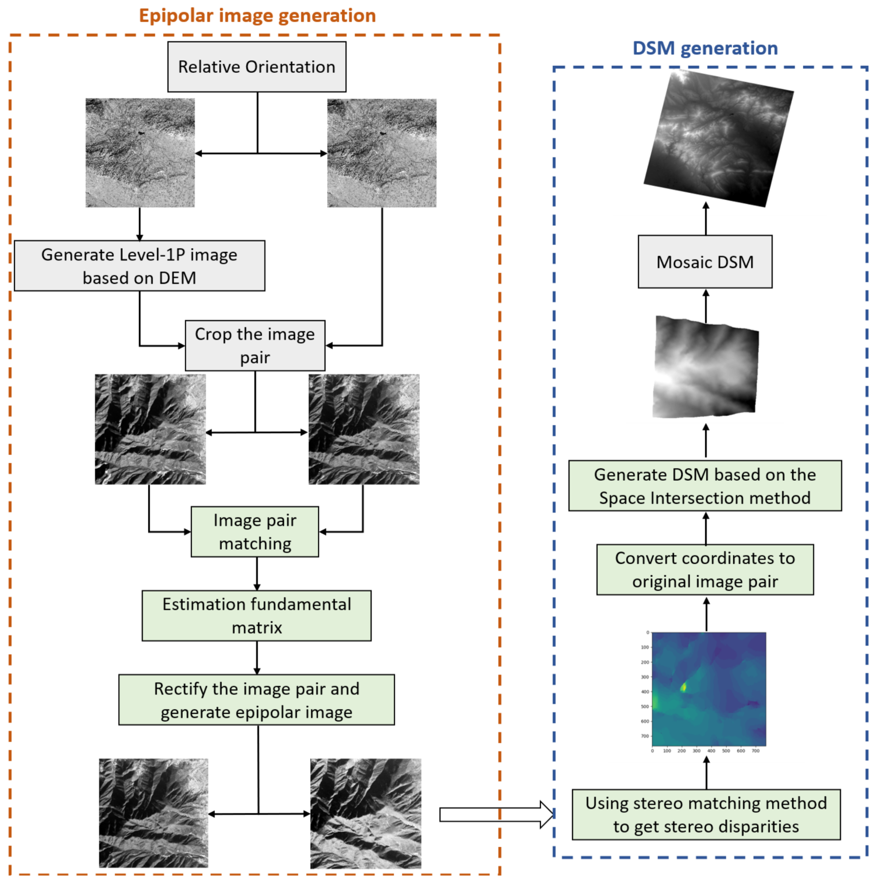
Based on the above analysis, we propose an approximate epipolar image generation framework that can be used for images in areas with large terrain undulations and multi-sensor images, such as SAR-SAR images and SAR-optical images. 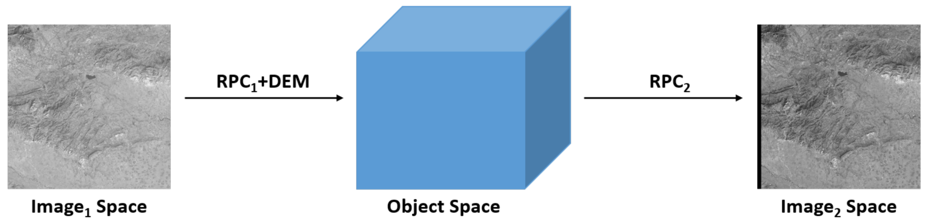By generating approximate epipolar images, the two-dimensional stereo matching problem is simplified to one-dimensional stereo matching, thereby improving the accuracy and efficiency of stereo matching [17]. Among them, the use of the digital elevation model (DEM) can reduce the initial offset of the two stereo images, thereby reducing the impact of terrain elevation changes on the generation of epipolar images. We first process the Level-1 images, which is the radiometric correction products, and use RPCs to project the left image into the image coordinate system of the right image to obtain a new image, which we name as Level-1P images, and then divide the entire image into blocks for parallel processing. Next, we generate approximate epipolar images and DSM for each block. Finally, all DSMs are spliced together to realize the generation of the whole DSM. The stereo satellite data used in this paper can be roughly divided into three categories. They are three-line array satellites, agile stereo satellites, and the general multiple view satellites. Three-line array satellites such as ZY-3 are equipped with three line-array cameras to image the same target from different angles along the direction of the satellite’s flight, to obtain the in-track stereo images [18]. Agile satellites (e.g., GeoEye) can maneuver in three directions: roll, pitch, and yaw [19]. By adjusting these three directions in a short period, agile satellites can realize nearly simultaneous multi-angle observations of the same target. The general multiple views satellites collect stereo images by taking images of the ground from different views, such as GF-2 and GF-3, and this kind of stereo image has no rigorous stereo property.

The rest of this paper is organized as follows. Section 2 first verifies the epipolar constraint relationship of single-sensor and multi-sensor images and then describes the proposed approximate epipolar image generation framework. In Section 3, the experimental results of epipolar image generation are shown, and their accuracy is qualitatively evaluated and quantitatively analyzed. In Section 4, DSM generation based on our proposed framework is discussed. Conclusions are drawn in Section 5.

2. Methods

In this section, we first describe the epipolar constraint relationship and investigate the theoretical epipolar constraints of single-sensor and multi-sensor images. It is proved that the epipolar curve of the optical image pair is hyperbolic, the epipolar constraint relationship of the SAR image pair is a quartic polynomial. Moreover, the epipolar constraint relationship of the optical-SAR image pair and SAR-optical are quadratic polynomial and high order polynomial, respectively. Then, we take GF-2 and GF-3 images as examples to verify the characteristics of the epipolar constraint relationship between the pushbroom optical image pairs and the SAR image pairs. It is proved that the epipolar curves of these images can be approximated as straight lines within the scope of the image scene, and they satisfy the conjugacy and approximate parallel properties. Finally, we propose a general epipolar image generation framework and introduce it in detail based on the epipolar constraint relationship.

2.1. Theory of the Multi-Sensor Epipolar Constraint

In conventional 3D reconstruction frameworks, the epipolar geometry is the first clarity constraint that facilitates the procedure of image matching by reducing the search space from 2D to 1D [2]. Usually, the images to be processed are created by resampling the original images according to epipolar geometry before dense matching, and the epipolarity constraint always exists for optical stereo images captured by frame type cameras that follow a perspective projection [17]. This principle is illustrated in Figure 1. The effective generation of epipolar-rectified images requires high positioning accuracy of the satellite sensor models, and thus a few ground control points (GCPs) are chosen to improve the positioning accuracy of the orientation parameters.

In the left view of the stereo pair, there is point $p_l$, which is the projection of the ground point P in the left image. If the point on the ray of point $p_l$ is projected into the right view through the image geometric model, the trajectory of these projection points forms the epipolar curve.

2.1.1. Epipolar Constraint of Optical Image Pairs

Supposing that the target P corresponds to two points $p_l$ and $p_r$ on the stereo pairs, and their image coordinates are denoted as $\left(x_l,y_l\right)$ and $\left(x_r,y_r\right)$. If the point $p_l$ is on the i-th scan line, and its coordinates on the focal plane can be denoted as $\left(0,p_l\right)$, there exists a relationship between the two coordinates [6]:

$$\begin{array}{c}{x}_l = i, y_l = \left(p_l+p_0\right)/\phantom{\left(p_l+p_0\right)e}e,\hfill \end{array}$$

(1)

where $p_0$ is the translation coefficient and e stands for the detector size. We can draw the following equation from the collinear relationship of the imaging geometry:

$$\left(\begin{array}{c}{X}_p\\ Y_p\\ Z_p\end{array}\right) = \left(\begin{array}{c}{X}_{S_i}\\ Y_{S_i}\\ Z_{S_i}\end{array}\right) + {\lambda }_i{R}_i\left(\begin{array}{c}0\\ p_l\\ -f\end{array}\right), R_i = \left(r_{im\times n}\right){}_{3\times 3},$$

(2)

where $\left(X_p,Y_p,Z_p\right)$ is the spatial coordinates of P, $\left(X_{S_i},Y_{S_i},Z_{S_i}\right)$ is the center of i-th scan line, $\lambda$ denotes the scale coefficient and $R_i$ denotes the rotation matrix, and f represents the focal length. We can also draw a similar relationship of point $p_r$:

$$\begin{array}{c}{x}_r=j\\ y_r = \left(p_r+p_0\right)/\phantom{\left(p_r+p_0\right)e}e\end{array}\&\left(\begin{array}{c}{X}_p\\ Y_p\\ Z_p\end{array}\right) = \left(\begin{array}{c}{X}_{S_j}\\ Y_{S_j}\\ Z_{S_j}\end{array}\right) + {\lambda }_j{R}_j\left(\begin{array}{c}0\\ p_r\\ -f\end{array}\right), R_j = \left(r_{jm\times n}\right){}_{3\times 3}.$$

(3)

Combining the two collinear equations of points $p_l$ and $p_r$, we can obtain

$$\left(\begin{array}{c}0\\ p_r\\ -f\end{array}\right) = \frac{1}{{\lambda }_j}{R_j}^{\prime }\left(\begin{array}{c}{X}_{S_i}-X_{S_j}\\ Y_{S_i}-Y_{S_j}\\ Z_{S_i}-Z_{S_j}\end{array}\right) + \frac{{\lambda }_i}{{\lambda }_j}{R_j}^{\prime }{R}_i\left(\begin{array}{c}0\\ p_l\\ -f\end{array}\right),$$

(4)

where ${R_j}^{\prime }$ is the inverse matrix of $R_j$, and it is denoted as ${R_j}^{\prime }= \left({r^{\prime }}_{jm\times n}\right){}_{3\times 3}$, and $R_{ij}={R_j}^{\prime }{R}_i={\left(r_{m\times n}\right)}_{3\times 3}.$ Assuming that the satellite is flying with high stability, the attitude remains unchanged during imaging, and thus the coordinates of the projection center can be regarded as a linear function that changes with the exposure time (scanning number), as follows:

$$\begin{array}{c}{X}_{S_i}=u_{1}i+u_2,Y_{S_i}=u_{3}i+u_4,Z_{S_i}=u_{5}i+u_6,\hfill \\ X_{S_j}=u_{7}j+u_8,Y_{S_j}=u_{9}j+u_{10},Z_{S_j}=u_{11}j+u_{12},\hfill \end{array}$$

(5)

where $u_1...u_{12}$ are the known imaging parameters. All variables except $\left(x_r,y_r\right)$ can be regarded as known variables, if we use the left image as the reference images. Substituting the above function into Equation (4), we can derive the epipolar curve on the right image, which refers to the relationship between $x_r$ and $y_r$ can be derived as follows:

$$e{y}_r-p_0=-f\frac{U_1{x}_r+U_2}{U_3{x}_r+U_4}\Rightarrow U_4{x}_r{y}_r+U_5{x}_r+U_6{y}_r+U_7=0,$$

(6)

where $U_k,k=1,2,...,7$ are the combinations of known variables. We can see from Equation (6) that the epipolar curve of two linear sensors is a hyperbolic curve.

2.1.2. Epipolar Constraint of SAR Image Pairs

The imaging geometry of SAR sensors is a side-looking model based on the Range-Doppler (RD) geometry which is different from the linear array model of optical sensors. Similar to the optical stereo pairs, the spatial coordinates and image coordinates of the target P also fulfill two imaging models [20],

$$\begin{array}{c}{\left(X_p-X_{S_i}\right)}^2+{\left(Y_p-Y_{S_i}\right)}^2+{\left(Z_p-Z_{S_i}\right)}^2={\left(R_i+M_i{y}_l\right)}^2\hfill \\ V_{X_i}\left(X_p-X_{S_i}\right) + V_{Y_i}\left(Y_p-Y_{S_i}\right) + V_{Z_i}\left(Z_p-Z_{S_i}\right) =-\frac{{\lambda }_i{f}_{dc}}{2}\left(R_i+M_i{y}_l\right),\hfill \\ {\left(X_p-X_{S_j}\right)}^2+{\left(Y_p-Y_{S_j}\right)}^2+{\left(Z_p-Z_{S_j}\right)}^2={\left(R_j+M_j{y}_r\right)}^2\hfill \\ V_{X_j}\left(X_p-X_{S_j}\right) + V_{Y_j}\left(Y_p-Y_{S_j}\right) + V_{Z_j}\left(Z_p-Z_{S_j}\right) =-\frac{{\lambda }_j{f}_{dc}}{2}\left(R_j+M_j{y}_r\right),\hfill \end{array}$$

(7)

where $\lambda$ is the radar wavelength, $f_{dc}$ denotes the Doppler shift parameter and is generally set to 0, R is the slant-range of the first range pixel, and M denotes the range sampling rate. $\left(X_S,Y_S,Z_S\right)$ and $\left(V_X,V_Y,V_Z\right)$ denote the position and velocity vectors of the antenna phase center, and the position vectors are polynomial functions of the velocity vectors, time and acceleration vectors. For the sake of simplification, the movement trajectory of SAR sensors is approximated as a linear model, as shown below:

$$\left\{\begin{array}{c}{X}_{S_i}=X_{S_{i0}}+V_{X_{i0}}k{x}_l\\ Y_{S_i}=Y_{S_{i0}}+V_{Y_{i0}}k{x}_l\\ Z_{S_i}=Z_{S_{i0}}+V_{Z_{i0}}k{x}_l\end{array}\right.,\left\{\begin{array}{c}{X}_{S_j}=X_{S_{j0}}+V_{X_{j0}}k{x}_r\\ Y_{S_j}=Y_{S_{j0}}+V_{Y_{j0}}k{x}_r\\ Z_{S_j}=Z_{S_{j0}}+V_{Z_{j0}}k{x}_r\end{array}\right.,$$

(8)

where k denotes the reciprocal of the pulse repetition frequency. We also assume all variables except $\left(x_r,y_r\right)$ are known parameters when taking the left image as the reference images. Combining two Doppler equations in Equation (7), we can obtain

$$\left(V_{X_i}{V}_{Z_j}-V_{X_j}{V}_{Z_i}\right)X_p= \left(V_{Y_j}{V}_{Z_i}-V_{Y_i}{V}_{Z_j}\right)Y_p+ \left(V_{X_i}{X}_{S_i}+V_{Y_i}{Y}_{S_i}+V_{Z_i}{Z}_{S_i}\right)V_{Z_j}- \left(V_{X_j}{X}_{S_j}+V_{Y_j}{Y}_{S_j}+V_{Z_j}{Z}_{S_j}\right)V_{Z_i}.$$

(9)

The above equation can be simplified as $X_p=v_1{Y}_p+v_2{x}_r+v_3.$ And from the Doppler equation of the left image, we can derive that

$$Z_p= \left(V_{X_i}{X}_{S_i}+V_{Y_i}{Y}_{S_i}+V_{Z_i}{Z}_{S_i}-V_{X_i}{X}_p-V_{Y_j}{Y}_p\right)/\phantom{\left(V_{X_i}{X}_{S_i}+V_{Y_i}{Y}_{S_i}+V_{Z_i}{Z}_{S_i}-V_{X_i}{X}_p-V_{Y_j}{Y}_p\right)V_{Z_i}}{V}_{Z_i}.$$

(10)

Substituting $Z_p$ and $X_p$ into the two Range equations in Equation (7), we can deduce

$$\begin{array}{c}{v}_{20}{Y}_P^2+ \left(v_{21}{x}_r+v_{22}\right)Y_p+v_{23}{x}_r^2+v_{24}{x}_r+v_{25}=0,\hfill \\ v_{26}{Y}_P^2+ \left(v_{27}{x}_r+v_{28}\right)Y_p+v_{29}{x}_r^2+v_{30}{x}_r+v_{31}={\left(R_j+M_j{y}_r\right)}^2.\hfill \end{array}$$

(11)

Removing $Y_p$ from the above equations, we can derive the final relationship between $\left(x_r,y_r\right)$ as follows, where $V_1...V_{13}$ are known variables, and it is a quartic polynomial.

$$V_1{y}_r^4+V_2{x}_r^4+V_3{x}_r^2{y}_r^2+V_4{x}_r^3+V_5{y}_r^3+V_6{x}_r{y}_r^2+V_7{x}_r^2{y}_r+V_8{x}_r^2+V_9{y}_r^2+V_{10}{x}_r{y}_r+V_{11}{x}_r+V_{12}{y}_r+V_{13}=0$$

(12)

2.1.3. Epipolar Constraint of Optical–SAR Image Pairs

As for the target P imaged by the pushbroom optical and the R-D SAR models, its imaging equations of the two stereo pairs can be described as follows [6,20]:

$$\begin{array}{c}\left(\begin{array}{c}{X}_p\\ Y_p\\ Z_p\end{array}\right) = \left(\begin{array}{c}{X}_{S_i}\\ Y_{S_i}\\ Z_{S_i}\end{array}\right) + {\lambda }_i{R}_i\left(\begin{array}{c}0\\ p_l\\ -f\end{array}\right),\begin{array}{c}{x}_l = i\hfill \\ y_l = \left(p_l+p_0\right)\hfill \end{array},\hfill \\ {\left(X_p-X_{S_j}\right)}^2+{\left(Y_p-Y_{S_j}\right)}^2+{\left(Z_p-Z_{S_j}\right)}^2={\left(R_j+M_j{y}_r\right)}^2,\hfill \\ V_{X_j}\left(X_p-X_{S_j}\right) + V_{Y_j}\left(Y_p-Y_{S_j}\right) + V_{Z_j}\left(Z_p-Z_{S_j}\right) = -\frac{{\lambda }_j{f}_{dc}}{2}\left(R_j+M_j{y}_r\right).\hfill \end{array}$$

(13)

From the linear array equation, we can obtain that

$$X_p=X_{S_i}+\frac{\left(r_{i12}{p}_l-r_{i13}f\right)}{\left(r_{i32}{p}_l-r_{i33}f\right)}\left(Z_p-Z_{S_i}\right),Y_p=Y_{S_i}+\frac{\left(r_{i22}{p}_l-r_{i23}f\right)}{\left(r_{i32}{p}_l-r_{i33}f\right)}\left(Z_p-Z_{S_i}\right).$$

(14)

Substituting $X_p$ and $Y_p$ into the Doppler equation of the right image, we can obtain $Z_p$ as

$$Z_p=\frac{\left[V_{X_j}\left(X_{S_j}-X_{S_i}\right) + V_{Y_j}\left(Y_{S_j}-Y_{S_i}\right) + V_{Z_j}{Z}_{S_j}\right]\left(r_{i32}{p}_l-r_{i33}f\right) + \left[V_{X_j}\left(r_{i12}{p}_l-r_{i13}f\right) + V_{Y_j}\left(r_{i22}{p}_l-r_{i23}f\right)\right]Z_{S_i}}{V_{X_j}\left(r_{i12}{p}_l-r_{i13}f\right) + V_{Y_j}\left(r_{i22}{p}_l-r_{i23}f\right) + V_{Z_j}\left(r_{i32}{p}_l-r_{i33}f\right)}.$$

(15)

We also assume that all variables except $\left(x_r,y_r\right)$ are known parameters when taking the left image as the reference image. Substituting $X_{S_j}=X_{S_{j0}}+V_{X_{j0}}k{x}_r,Y_{S_j}=Y_{S_{j0}}+V_{Y_{j0}}k{x}_r,Z_{S_j}=Z_{S_{j0}}+V_{Z_{j0}}k{x}_r$ into $Z_p$, we find out that $Z_p$ is a linear function of $x_r$,

$$Z_p=w_1+w_2{x}_r.$$

(16)

Similarly, $X_p$ and $Y_p$ are also linear functions of $x_r$, denoted as

$$X_p=w_3+w_4{x}_r,Y_p=w_5+w_6{x}_r.$$

(17)

Substituting $X_p,Y_p,Z_p$ into the Range equation, we can deduce

$$w_7{x}_r^2+w_8{x}_r+w_9{y}_r^2+w_{10}{y}_r+w_{11}=0,$$

(18)

and it is clear that the epipolar curve is a quadratic curve.

2.1.4. Epipolar Constraint of SAR-Optical Image Pairs

The epipolar geometries between optical-SAR pairs and SAR-optical pairs are also different since the optical and SAR imaging models are different. As for the target P imaged by the R-D SAR model and the pushbroom optical model, its imaging equations of the two stereo pairs can be described as follows [6,20]:

$$\begin{array}{c}{\left(X_p-X_{S_i}\right)}^2+{\left(Y_p-Y_{S_i}\right)}^2+{\left(Z_p-Z_{S_i}\right)}^2={\left(R_i+M_i{y}_l\right)}^2,\hfill \\ V_{X_i}\left(X_p-X_{S_i}\right) + V_{Y_i}\left(Y_p-Y_{S_i}\right) + V_{Z_i}\left(Z_p-Z_{S_i} \right)=-\frac{{\lambda }_i{f}_{dc}}{2}\left(R_i+M_i{y}_l\right),\hfill \\ \left(\begin{array}{c}{X}_p\\ Y_p\\ Z_p\end{array}\right) = \left(\begin{array}{c}{X}_{S_j}\\ Y_{S_j}\\ Z_{S_j}\end{array}\right) + {\lambda }_j{R}_j\left(\begin{array}{c}0\\ p_r\\ -f\end{array}\right),\begin{array}{c}{x}_r = j\hfill \\ y_r = \left(p_r+p_0\right)\hfill \end{array}.\hfill \end{array}$$

(19)

Following the derivation procedure of Section 2.1.3, and by assuming that all variables except $\left(x_r,y_r\right)$ are known parameters, we can obtain the relationship between $x_r,y_r$ as a high-order polynomial:

$$\begin{array}{c}{d}_{21}{x}_r^2{y}_r^4+d_{22}{x}_r{y}_r^4+d_{23}{x}_r^2{y}_r^3+d_{24}{y}_r^4+d_{25}{x}_r{y}_r^3+d_{26}{x}_r^2{y}_r^2+d_{27}{y}_r^3+d_{28}{x}_r^2{y}_r\hfill \\ +d_{29}{x}_r{y}_r^2+d_{30}{x}_r^2+d_{31}{y}_r^2+d_{32}{x}_r{y}_r+d_{33}{x}_r+d_{34}{y}_r+d_{35}=0.\hfill \end{array}$$

(20)

2.1.5. Verification of the Properties of Epipolar Constraint

As the rational function model can be regarded as an accurate alternative for rigorous imaging models for both optical and SAR images, we hereafter use RPCs for the sake of simplicity. For stereo images, the point $p_l$ in the left image can be projected to the object space by backward mapping using RPCs. By changing the elevation H, we can get the projected light in the object space. Then, using the RPCs of the right image to project the light into the right image, we can obtain the projection trajectory curve l. l is the epipolar curve corresponding to the point $p_l$. Moreover, the conjugate point of $p_l$ in the right image will be on the curve l. This method of generating epipolar curves is known as the projection trajectory method (PTM) [21]. Then, we use PTM to verify the epipolar curve is a hyperbolic curve for optical acquisitions with pushbroom model, a quartic curve for SAR acquisitions with Range–Doppler model, and the epipolar curves of the optical–SAR image pair and the SAR–optical image pair satisfy the quadratic polynomial and the high order polynomial, respectively. In addition, we also further verify other properties for multi-sensor models. We first choose a point in the left image, set its height range to [−500 m:9000 m] which is set based on the altitude of the Earth’s surface, then we get a series of points in the object space and map them to the right image. Finally, we use different functions to fit the epipolar curve.

Figure 2 shows the epipolar curves generated from the optical satellite (GF-2) image pairs and the SAR satellite (GF-3) image pairs using the PTM. From this figure, we can find that the epipolar curves of the GF-2 image pairs and GF-3 image pairs are similar to straight lines. This means that within the scope of the image scene, the epipolar curve can be approximated as a straight line. To further verify the shape of the epipolar curve, we fit the coordinates of the points in the projection trajectory. The fitting results are shown in Figure 3, Figure 4, Figure 5 and Figure 6.

The fitting results in Figure 3a show that when a linear function is used to fit the epipolar curve of the GF-2 image pair, the fitting residual can reach 3 pixels. However, when the fitting function is changed to a hyperbolic curve, the fitting residual is reduced by ~80%. Therefore, the epipolar curve of the optical image pair can be approximated as a hyperbolic curve, which is in accordance with the theoretical conclusion. As shown in Figure 4, for the GF-3 image pair, the quartic curve fitting residual of the epipolar curve is only approximately $1/50$ of the linear fitting residual. This means that the epipolar curve of the SAR image pair can be approximated by a quartic curve. For the optical-SAR image pair, when using linear fitting to fit the projection points, the fitting residual is between −25 and 8, which is shown in Figure 5a. However, the residual is within 1 pixel, if a quadratic polynomial is used for fitting. The results in Figure 6 show that by comparing the fitting residuals, the epipolar curve of the SAR–optical image pair can be approximated as a high order polynomial curve. These prove that the epipolar constraint relationship of the image pairs we derived is effective.

In addition, we also verify the conjugacy of the epipolar curves. Conjugacy means that the corresponding points are located on the corresponding epipolar curves, and the points on the corresponding epipolar curves correspond one to one. We select six points (Point 1–6) from the same epipolar curve in Figure 2b and calculate the corresponding epipolar curve of each point in Figure 2a. As the epipolar curve can be approximated as a straight line in a local range, for the convenience of calculation, we perform linear fitting on the epipolar curves of the six points in the left image. The result is shown in Figure 7a. From the linear fitting results, it can be found that the epipolar curves fitted by these 6 points are not the same line, which indicates that there is no strict epipolar curve pair in the stereo images obtained by the linear pushbroom camera. However, the partial magnified image demonstrates that the difference between the fitting results of the epipolar curves at different points is very small, within 0.1 pixels. Therefore, within the scope of the image scene, these points’ epipolar curves can be approximately regarded as the same epipolar curve, that is, the epipolar curves satisfy the conjugacy in the image range. Next, we verify the approximate parallel property of the epipolar curves. In Figure 2a, we randomly select 4 points and perform a linear fitting on the projection trajectory of each point in Figure 2b. The linear fitting results are shown in Figure 7b. Figure 7b indicates that the linear fitting slopes of the epipolar curves corresponding to these four points are approximately equal, which means that the epipolar curves have the parallel property in the image range.

2.2. The Proposed General Epipolar Image Generation Framework

Based on the epipolar constraint relationship deduced in Section 2.1, we then introduce the proposed framework. Our framework can be divided into the following steps: (1) image pairs relative orientation, (2) image spatial conversion and overlapping region extraction based on DEM, (3) cropping the image pairs into small patches, (4) matching stereo image pairs based on spatial structure features and three-dimensional phase correlation algorithm, (5) estimating the fundamental matrix F based on the matching points, (6) image pairs correction and generate epipolar images, (7) calculating the coordinates in the original image and generate DSM using space intersection method, and (8) mosaic DSM. The flowchart of the proposed framework is presented in Figure 8. Next, we will introduce our framework in detail.

We first preprocess the input Level-1 images, that is, we perform the relative orientation between image pairs. The relative orientation takes the principle that the corresponding rays are coplanar as the theoretical basis to restore or determine the relative positional relationship of the image pairs during imaging. The principle is to construct the conditional expression of the relative orientation elements based on the intersecting characteristic of the light pair corresponding to the stereo pair and solve the relative orientation elements by formulating equations [22]. We denote the preprocessed left and right images as $Imag{e}_1$ and $Imag{e}_2$, respectively. Then, we generate epipolar images and DSM from $Imag{e}_1$ and $Imag{e}_2$.

2.2.1. Image Spatial Conversion and Overlapping Region Extraction Based on DEM

The rational function model is a generalized sensor model that can replace the linear array pushbroom camera model and the SAR physical camera model [14]. This model makes full use of the auxiliary parameters of satellite imagery and solves the model coefficients by fitting with the existing strict geometric model. Because of the high accuracy of the rational polynomial coefficients, it is widely used in line array optical satellites. Therefore, our framework is based on the RPCs to perform image space conversion and overlapping region extraction on stereo images. The RFM expresses the image space coordinates $\left(r,c\right)$ as a polynomial ratio of the object space coordinates $\left(X,Y,Z\right)$, which is shown in Equation (21).

$$\begin{array}{c}\hfill r_n=\frac{P_1\left(X_n,Y_n,Z_n\right)}{P_2\left(X_n,Y_n,Z_n\right)},c_n=\frac{P_3\left(X_n,Y_n,Z_n\right)}{P_4\left(X_n,Y_n,Z_n\right)},\end{array}$$

(21)

where $P_1$, $P_2$, $P_3$, and $P_4$ are polynomials, and $r_n$, $c_n$, $X_n$, $Y_n$, and $Z_n$ are normalized coordinates.

According to Equation (21), the corresponding image coordinates can be calculated according to the latitude, longitude, and elevation of a certain point in the object space. This process is called the RPCs positive solution. In addition, the RPCs inverse solution calculation formulas are as follows:

$$\begin{array}{c}\hfill X_n=\frac{P_5\left(r_n,c_n,Z_n\right)}{P_6\left(r_n,c_n,Z_n\right)},Y_n=\frac{P_7\left(r_n,c_n,Z_n\right)}{P_8\left(r_n,c_n,Z_n\right)},\end{array}$$

(22)

where $P_5$, $P_6$, $P_7$, and $P_8$ are polynomials. For the RPCs positive solution, by substituting the latitude and longitude coordinates and elevation into Equation (21), the row and column coordinates in the image space can be obtained. However, when $\left(r,c\right)$ is known and uses the RPCs inverse solution formulas to calculate the spatial coordinates, it cannot be solved directly due to a lack of elevation information. Therefore, it is necessary to combine the DEM to obtain the corresponding spatial coordinates through multiple iterations, that is the Ray Tracing method combined with DEM from the image space to the object space [23].

Therefore, we first use RPCs to perform spatial conversion and overlapping region extraction on stereo satellite images based on DEM to obtain processed image pairs. For ease of description, we denote the RPCs corresponding to $Imag{e}_1$ and $Imag{e}_2$ as $RP{C}_1$ and $RP{C}_2$. The schematic diagram of the image space conversion processing flow is shown in Figure 9. The specific steps are as follows:

• For each pixel in $Imag{e}_1$, substitute the row and column coordinates into Equation (22) according to $RP{C}_1$. The corresponding object space longitude, latitude, and elevation are iteratively calculated using the ray tracing method.
• Substituting the spatial coordinates obtained in the previous step into Equation (21) constructed by $RP{C}_2$, the coordinates in the image space of $Imag{e}_2$ corresponding to the object points can be obtained.
• According to the corresponding relationship between the image space of $Imag{e}_1$ and the image space of $Imag{e}_2$, the new left image, which is called Level-1P image and denoted as $Imag{e}_{1P}$, is obtained. $Imag{e}_{1P}$ only contains the overlapping area of the image pair. Then, $Imag{e}_{1P}$ and $Imag{e}_2$ are used as a new image pair to generate epipolar images and DSM.

Figure 9. The schematic diagram of the image space conversion process.

Figure 9. The schematic diagram of the image space conversion process.

2.2.2. Image Blocks Dividing in $Imag{e}_{1P}$ and $Imag{e}_2$

We divide the image pairs into several square image block pairs to improve the accuracy and speed of epipolar images and DSM generation. We crop an image block every 512 pixels when dividing image blocks, so that adjacent image blocks have a 50% overlap area, to ensure that the final generated DSM can cover all areas of the image. The image blocks covering the same area in $Imag{e}_{1P}$ and $Imag{e}_2$ are respectively denoted as $im{g}_1$ and $im{g}_2$. By dividing the image pairs into several block pairs, it is helpful to extract more reliable conjugate features and increase the efficiency. The block size is set to 1024 × 1024 pixels, which can maintain the affine transformation characteristics [24].

2.2.3. Images Matching Based on Spatial Structure Features and 3D Phase Correlation

Considering the radiometric and geometric distortions caused by view conditions and sun angles, herein, we use a robust feature matching method to obtain high-precision correspondences. Based on our previous work [25], we extract intensity-invariant and sensor-invariant structure features and put them into the 3D phase correlation framework. Traditional phase correlation methods are based on two core ideas. The first is the assumption of brightness constancy, that is, the intensity of pixels in an image with a certain offset remains unchanged. The second is the famous Fourier transform characteristic, which means that the Fourier phases of two functions that have an offset in the spatial domain have a linear difference. These two core ideas are given as follows:

$$I_1\left(x,y\right) =I_2\left(x-x_0,y-y_0\right),F_1\left(u,v\right) =F_2\left(u,v\right)exp\left\{-2\pi i\left(u{x}_0+v{y}_0\right)\right\},$$

(23)

where $I_1$ and $I_2$ are two images, $F_1$ and $F_2$ are the corresponding Fourier Transforms, and $x_0$ and $y_0$ are the offsets of the coordinates. The normalized cross power spectrum can be obtained:

$$Q\left(u,v\right) =\frac{F_1\left(u,v\right)F_2{\left(u,v\right)}^{*}}{\left|F_1\left(u,v\right)F_2{\left(u,v\right)}^{*}\right|}=exp\left\{-2\pi i\left(u{x}_0+v{y}_0\right)\right\}.$$

(24)

The inverse Fourier transform of the cross power spectrum is the impulse function in the spatial domain. By locating the extreme points in the spatial domain, the offsets in the two directions can be found:

$$\mathrm{Q}\left(x,y\right) =\delta \left(x-x_0,y-y_0\right)$$

(25)

However, for multi-view and multi-sensor remote sensing images, there are often radiation and geometric differences between them, which make the first core idea of the phase correlation method no longer applicable. To solve this problem, we first map the input images to a feature space, which retains the invariance by capturing the inherent structural information. Two three-dimensional feature sets are formed and embedded in the three-dimensional phase correlation process to estimate the two-dimensional translational displacement by using dense spatial structure feature representation instead of image intensity.

For spatial structure features, we use dense scale invariant transform features [26]. First, we calculate the horizontal and vertical gradient response of each pixel. Then, we obtain the histogram structure of the gradient position and direction based on the gradient magnitude and direction to construct the spatial feature. Finally, we embed two 3-D feature images into the 3-D phase correlation process, as shown below:

$$V_1\left(x,y,g\right) =V_2\left(x-x_0,y-y_0,g\right),$$

(26)

where $V_1$ and $V_2$ are two 3-D feature images. x and y are the coordinates of the pixels in the image. g represents the gradient magnitude of the pixel. The Fourier translation characteristics of the 3-D phase correlation are

$$\mathcal{F}\left\{V_2\left(x-x_0,y-y_0,g\right)\right\} =e^{-2\pi i\left(u{x}_0+v{y}_0\right)}\mathcal{F}\left\{V_2\left(x,y,g\right)\right\}.$$

(27)

The normalized cross power spectrum of the above equation is

$$\begin{array}{cc}\hfill Q\left(u,v,w\right)& =\frac{F_1\left(u,v,w\right)F_2{\left(u,v,w\right)}^{*}}{\left|F_1\left(u,v,w\right)F_2{\left(u,v,w\right)}^{*}\right|}=exp\left\{-2\pi i\left(u{x}_0+v{y}_0\right)\right\}\overrightarrow{d},\hfill \end{array}$$

(28)

where $F_1$ and $F_2$ are the three-dimensional Fourier transforms corresponding to $V_1$ and $V_2$. $\overrightarrow{d}$ is a three-dimensional unit vector, and its direction is the direction of the gradient of the pixel. The three-dimensional inverse Fourier Transform of Equation (28) is an impulse function throughout three-dimensional space:

$$\mathrm{Q}\left(x,y,g\right) ={\mathcal{F}}^{-1}\left\{Q\left(u,v,w\right)\right\} =\delta \left(x-x_0,y-y_0\right)\overrightarrow{d}$$

(29)

The biggest difference between $\mathrm{Q}\left(x,y,g\right)$ and $\mathrm{Q}\left(x,y\right)$ is that we need to locate the impulse response in three-dimensional space instead of two-dimensional space. A simple and direct method is to sum the third dimension information in $\mathrm{Q}\left(x,y,g\right)$ and convert it into $\mathrm{Q}\left(x,y\right)$ to solve. Finally, two-dimensional translational displacement can be estimated by locating the maximum response, and then correspondences are obtained.

2.2.4. Fundamental Matrix Estimation Based on Conjugation Points

In Section 2.1, we introduced the epipolar constraint relationship between image pairs. The epipolar constraint can also be expressed in mathematical form, that is, the fundamental matrix. The fundamental matrix F represents the mapping from $p_l$ in the left image to the epipolar curve $l_r$ in the right image. This relationship is expressed as $l_r=F{p}_l$ [27].

Based on the epipolar constraint, the corresponding right image point $p_r$ must be on the epipolar curve $l_r$, and

$$p_r^T{l}_r=p_r^{T}F{p}_l=0.$$

(30)

When the coordinates of the matching points in the image pairs are obtained from the aforementioned feature matching method, combined with Equation (30), F between the image pairs can be calculated. As F is a $3\times 3$ matrix with 9 unknowns in total, at least eight pairs of matching points are required to solve F. Therefore, we use the Eight-Point-Algorithm to calculate F [28].

2.2.5. Image Pairs Correction Based on Fundamental Matrix

Combining the matching points of the left and right images $im{g}_1$ and $im{g}_2$, and the fundamental matrix F, the image pairs can be corrected to generate epipolar images. In this paper, we use the Hartley method [29] to correct the image pairs. This method can be implemented in two steps.

First of all, we need to calculate the projection transformation matrices $H_l$ and $H_r$ based on the fundamental matrix [30] and this method is the same as the epipolar rectification technique of the Ames Stereo pipeline [31]. The projection transformation matrix H can be obtained by multiplying four matrices, that is, $H=CGRT$. The four matrices C, G, R, and T, respectively, represent different transformation relations. We assume that the homogeneous coordinates of the pole of the right image is ${\left(u_e,v_e,1\right)}^T$, and the homogeneous coordinates of the center point of the right image is ${\left(u_c,v_c,1\right)}^T$. Then, we can obtain the projection transformation matrix $H_r$ corresponding to the right image as follows:

$$H_r=CGRT=\left[\begin{array}{ccc}1& 0& u_c\\ 0& 1& v_c\\ 0& 0& 1\end{array}\right]\left[\begin{array}{ccc}1& 0& 0\\ 0& 1& 0\\ -\frac{1}{u_e^2}& 0& 1\end{array}\right]\left[\begin{array}{ccc}\frac{u_e^1}{\sqrt{{\left(u_e^1\right)}^2+{\left(v_e^1\right)}^2}}& \frac{v_e^1}{\sqrt{{\left(u_e^1\right)}^2+{\left(v_e^1\right)}^2}}& 0\\ -\frac{v_e^1}{\sqrt{{\left(u_e^1\right)}^2+{\left(v_e^1\right)}^2}}& \frac{u_e^1}{\sqrt{{\left(u_e^1\right)}^2+{\left(v_e^1\right)}^2}}& 0\\ 0& 0& 1\end{array}\right]\left[\begin{array}{ccc}1& 0& -u_c\\ 0& 1& -v_c\\ 0& 0& 1\end{array}\right],$$

(31)

where ${\left(u_e^1,v_e^1,1\right)}^T=T{\left(u_e,v_e,1\right)}^T$ and ${\left(u_e^2,v_e^2,1\right)}^T=R{\left(u_e^1,v_e^1,1\right)}^T$.

Assuming that among the N pairs of matching points obtained in the Section 2.2.3, the coordinates of the i-th pair of matching points in the left and right images are $p_1^i={\left(u_1^i,v_1^i\right)}^T$ and $p_2^i={\left(u_2^i,v_2^i\right)}^T$, respectively. Then, $H_l$ can be computed by the following equation, where d denotes the distance between $H{p}_1^i$ and $H_r{p}_2^i$.

$$H_l=\underset{H}{arg}min\sum _{i=1}^{N}d{\left(H{p}_1^i,H_r{p}_2^i\right)}^2.$$

(32)

Second, we resample the pair of image blocks $im{g}_1$ and $im{g}_2$ after calculating the projection transformation matrices $H_l$ and $H_r$. We assume that these two matrices $H_l$ and $H_r$ can map vectors to the same plane J. Moreover, in the plane J, there is a window W with a size of 1024 × 1024 pixels. Then, $im{g}_1$ and $im{g}_2$ can be resampled through $H_1$ and $H_r$, so that the resampled two images are within the range of window W. For any point $p^{\prime }$ in W, its corresponding point in $im{g}_1$ can be expressed as $p_l=H_l^{-1}{p}^{\prime }$. Similarly, the corresponding point of $p^{\prime }$ in $im{g}_2$ is $p_r=H_r^{-1}{p}^{\prime }$. Then, $im{g}_1$ and $im{g}_2$ can be resampled to the window W in plane J which are denoted as $im{g}_1^{\prime }$ and $im{g}_2^{\prime }$, through bicubic interpolation.

Finally, we crop the middle part from $im{g}_1^{\prime }$ and $im{g}_2^{\prime }$ as the final epipolar images, denoted as $ep\_im{g}_1$ and $ep\_im{g}_2$.

2.3. DSM Generation

We use Semi-Global Matching (SGM) [32] which was proposed by Hirschmüller to obtain pixelwise matching points from $ep\_im{g}_1$ and $ep\_im{g}_2$. The realization process of the stereo matching algorithm can be summarized into the following four steps: matching cost calculation, matching cost aggregation, disparity calculation, and disparity optimization [33].

We set the left epipolar image $ep\_im{g}_1$ as the reference image, after obtaining the disparity map of the image pair based on the stereo matching method. Through the back-projection transformation, we calculate the coordinates of each pixel in $ep\_im{g}_1$ and $ep\_im{g}_2$ in $Imag{e}_{1P}$ and $Imag{e}_2$, respectively; their coordinates are denoted as $\left(u_{1p},v_{1p}\right)$ and $\left(u_2,v_2\right)$. It is necessary to convert the coordinates in $Imag{e}_{1P}$ to the coordinates in the original image $Imag{e}_1$ in order to further generate DSM. We substitute $RP{C}_2$ into Equation (22) and use the ray tracing method based on DEM to calculate the spatial coordinates $\left(X,Y,Z\right)$ corresponding to $\left(u_{1p},v_{1p}\right)$. Then, by substituting $\left(X,Y,Z\right)$ into Equation (21) formed by $RP{C}_1$, we obtain the corresponding coordinates of $\left(u_{1p},v_{1p}\right)$ in $Imag{e}_1$. Finally, we can produce DSM based on the space forward intersection method.

3. Results

In this section, we first evaluate the performance of the proposed framework by comparing it to the current state-of-the-art algorithms. The first method is an epipolar image generation algorithm based on the PTM [21]. The second method is the S2P method [24]. Various scenarios of different sensors, including urban, agriculture, and mountain areas, are used. Then, we explore the applicability of our framework on SAR–optical and SAR–SAR image pairs. In the comparative experiment, the disparities of the matching points are used as the quantitative metric to evaluate the quality of the generated epipolar images. The satellite images used in our experiment include ZY-3, GF-2, GF-3, and GeoEye images. Among them, ZY-3, GF-2, and GeoEye are optical satellites, and GF-3 is a SAR satellite. The coverage area of these image data and their information are shown in

Table 1. The information of the satellite image pairs. GSD represents the ground sampling distance.

Stereo Image Pair		GSD	Area	Topographic Feature
ZY-3	Left	3.5 m	Songshan	Mountainous
	Right	3.5 m
ZY-3	Left	3.5 m	Tianshan	Mountainous
	Right	3.5 m
GeoEye	Left	0.5 m	Omaha	Urban
	Right	0.5 m
GF-3	Left	1 m	Omaha	Urban
	Right	1 m
GF-3	Left	1 m	Songshan	Mountainous
GF-2	Right	0.8 m

.

3.1. Experimental Results of Epipolar Images Generation

To verify the performance of the proposed approximate epipolar image generation framework, we first select the ZY-3 satellite images of the Songshan area in China, which is mostly mountainous. The elevation range of Songshan is approximately 67–1472 m. In order to further verify the performance of our framework, the results obtained by our framework are compared to two other methods.

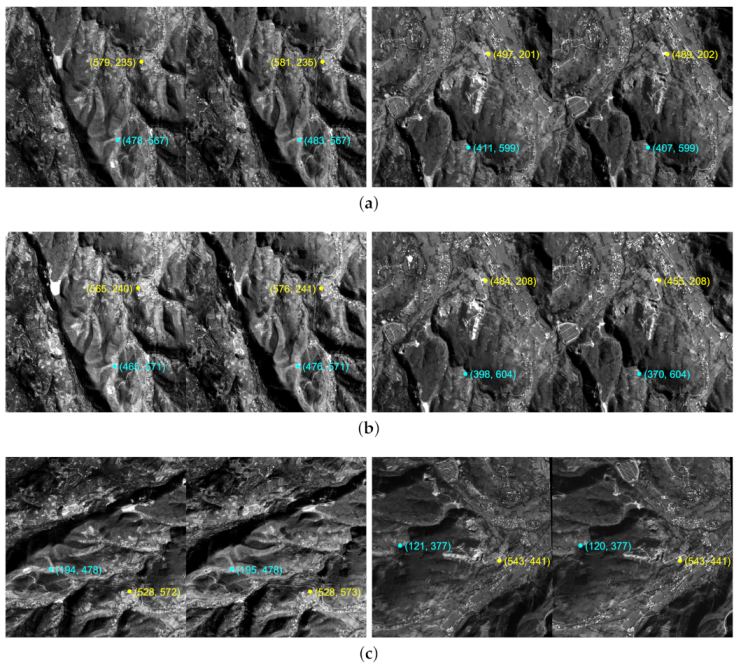
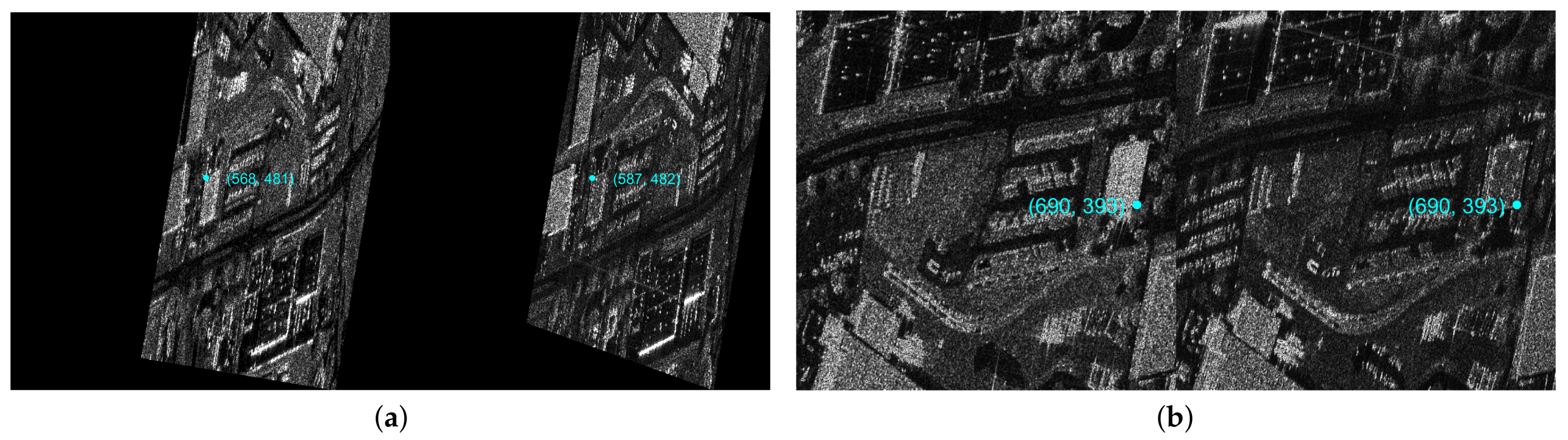
The epipolar images generated by the proposed framework is shown in Figure 10c. From the results, it can be found that the vertical disparity of the generated epipolar image pair is approximately negligible, which means that satisfactory results can be obtained for areas with large terrain elevation changes that do not satisfy the affine transformation model. In addition, the epipolar images generated by two other comparison methods in the same region are shown in Figure 10a,b. In order to make the comparison of results more intuitive, we manually select two corresponding points in the epipolar images and display their coordinates $(x,y)$, where x is the horizontal coordinate and y is the vertical coordinate. The results show that the y-disparity of the epipolar images generated by these three methods is relatively small and can be approximately ignored. However, in addition to the y-disparity, the x-disparity of the points in Figure 10c is almost negligible. Therefore, it is clear that compared with the other two methods, the proposed framework can get better epipolar images.

We further calculate the y-disparity of the SIFT matching points in the epipolar image pair to quantitatively evaluate the results. The smaller this y-disparity, the higher the accuracy of the generated epipolar images. Moreover, when performing stereo matching, the reduction of the search range of matching points will improve the accuracy and efficiency of image matching. Therefore, we also calculate the x-disparity of the SIFT matching points at the same time. When the x-disparity is small, the matching efficiency and accuracy during dense matching of epipolar images will be improved. The disparity of matching points is shown in

Table 2. The disparity of the matching points in the epipolar images in Songshan. Max and Mean represent the maximum and average values of disparity, respectively. $\sigma$ represents the standard deviation relative to the average disparity.

Satellite	Area	Method	y-Disparity (Pixels)			x-Disparity (Pixels)
			Max	Mean	$\mathit{\sigma }$	Max	Mean	$\mathit{\sigma }$
ZY-3	Mountainous Area-1	S2P	2	0.48	0.54	14	5.97	4.01
		PTM	3	0.59	0.57	15	6.64	3.26
		Ours	3	0.28	0.50	2	0.61	0.60
	Mountainous Area-2	S2P	3	0.79	0.63	21	9.31	5.63
		PTM	2	0.74	0.60	15	5.96	4.90
		Ours	3	0.60	0.66	4	0.82	0.81
	Mountainous Area-3	S2P	2	0.74	0.56	18	9.36	4.74
		PTM	4	0.66	0.68	35	13.86	8.29
		Ours	3	0.61	0.75	3	0.60	0.60

. For the sake of comparison, the data in the tables are the statistical results of the absolute value of the disparity.

It can be found that the proposed framework can generate high-quality epipolar images in regions with large terrain undulations according to the image matching results. For the y-disparity, the results obtained by our framework are slightly smaller than the results obtained by the S2P and PTM-based methods. Although the proposed framework only shows a small advantage in y-disparity, it has obvious advantages in x-disparity. The epipolar images obtained by our framework also have higher similarity in the x-direction and the average x-disparity of the matching points can reach the sub-pixel level. The results show that the epipolar images generated by our framework can rearrange the original images better so that the corresponding points of the image pair are approximately on the same horizontal line, thereby reducing the search range of conjugate points in image matching to 1-D space. In addition, the generated epipolar images can also reduce the disparity in the x-direction, which provides a guarantee for the efficiency and accuracy of the dense matching before the subsequent DSM generation.

We also conduct experiments on ZY-3 images in Tianshan, China, which are shown in Figure 11. Compared with the Songshan area, the terrain changes in this area are more obvious, approximately 24–3091 m. The quality of the epipolar images generated in this area is quantitatively evaluated, and the results are shown in

Table 3. The disparity of the matching points in the epipolar images in Tianshan.

Satellite	Area	Method	y-Disparity (Pixels)			x-Disparity (Pixels)
			Max	Mean	$\mathit{\sigma }$	Max	Mean	$\mathit{\sigma }$
ZY-3	Mountainous Area-1	S2P	3	0.48	0.88	75	7.13	14.75
		PTM	3	0.50	0.73	30	13.79	5.58
		Ours	4	0.71	0.98	11	2.59	2.61
	Mountainous Area-2	S2P	1	0.63	0.48	47	19.75	11.96
		PTM	1	0.33	0.47	63	17.20	18.40
		Ours	1	0.33	0.47	10	1.60	1.65

. Compared with the Songshan area, the elevation of the Tianshan area has greater fluctuations, so the x-disparity of the generated epipolar image will be greater. However, by comparing the results of the other two methods, it can be found that the x-disparity of the epipolar image generated by the proposed framework is still optimal among the three methods. The results show that in areas with large elevation fluctuations, not only the y-disparity can reach sub-pixels in the epipolar images generated by our framework, but most of the average x-disparity does not exceed 3 pixels. Therefore, our epipolar image generation framework has more obvious advantages for areas with large undulations like Tianshan.

3.2. Verification of the Applicability of the Proposed Framework

It has been verified in Section 3.1 that the proposed framework can generate good epipolar images for areas with large terrain elevation changes. We select stereo image pairs from other satellites and other regions to generate epipolar images to verify the applicability of the proposed framework.

3.2.1. The Results of Epipolar Image Generation for Different Terrains

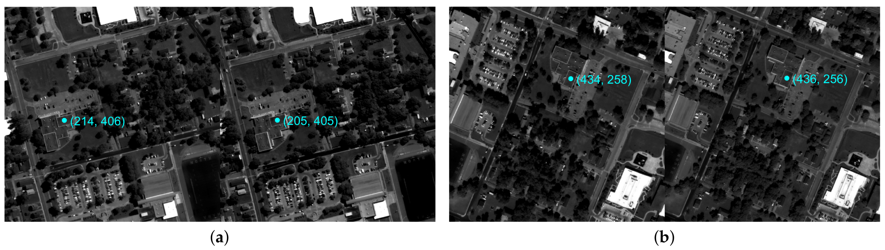
We choose the Omaha region of the United States to verify the applicability of the proposed framework in regions with small terrain undulations. The results of the comparative experiment are shown in Figure 12 and

Table 4. The disparity of the matching points of the epipolar images in Omaha.

Satellite	Area	Method	y-Disparity (Pixels)			x-Disparity (Pixels)
			Max	Mean	$\mathit{\sigma }$	Max	Mean	$\mathit{\sigma }$
GeoEye	Urban Area-1	S2P	2	0.60	0.57	18	9.06	4.65
		Ours	3	1.30	0.96	5	1.17	1.12
	Urban Area-2	S2P	3	1.46	0.54	12	10.43	1.40
		Ours	3	1.02	0.81	4	1.56	0.81

. The results show that the proposed framework can still achieve ideal results for urban areas with smaller terrain undulations and larger elevation gradients than mountain areas. Compared with the S2P method, the proposed framework has no obvious advantages for the y-disparity of the epipolar image in the urban area. But the x-disparity is still relatively small. The mean values of the x-disparity of the corresponding points are both about 1 to 2 pixels. Therefore, the proposed epipolar image generation framework is also applicable to areas with small terrain undulations and large terrain undulation gradients.

3.2.2. The Results of Epipolar Image Generation for Different Sensors

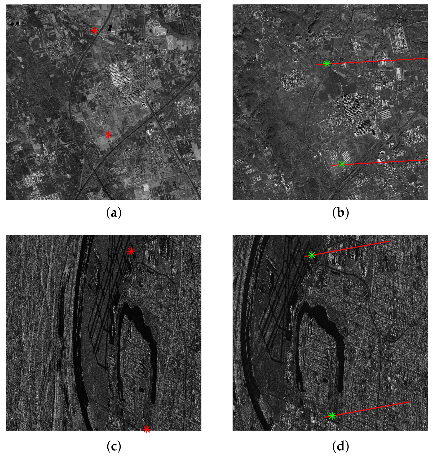
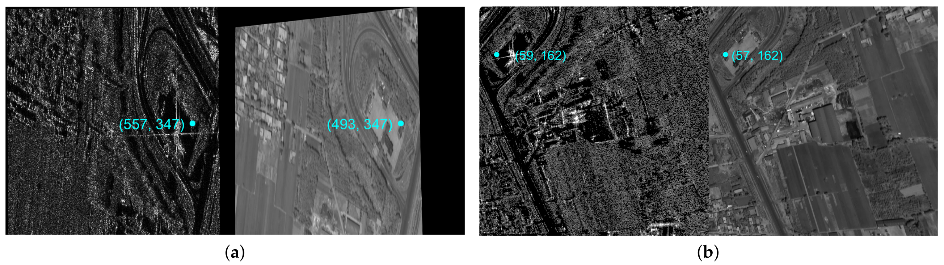
We conduct experiments on satellite images from other sources to further verify the universality of the proposed epipolar image generation framework. We choose the stereo image pair consisting of GF-3 satellite image and GF-2 satellite image in Songshan in this experiment. We first generate epipolar images based on the SAR-optical image pair. Due to the particularity of SAR imaging, we adopt different structural features in the matching stage for SAR images [25]. The epipolar images obtained using the proposed framework are shown in Figure 13. The average y-disparity of the image matching points can reach approximately 1 pixel, and the average x-disparity is less than 2 pixels (see

Table 5. The disparity of matching points in the epipolar images generated by the GF-3–GF-2 image pair in Songshan.

Satellite	Area	Method	y-Disparity (Pixels)			x-Disparity (Pixels)
			Max	Mean	$\mathit{\sigma }$	Max	Mean	$\mathit{\sigma }$
GF-3 and GF-2	Urban Area-1	S2P	19	2.48	3.64	78	60.20	7.37
		Ours	6	1.18	1.09	7	1.85	1.51
	Urban Area-2	S2P	7	1.14	1.72	66	62.74	3.39
		Ours	4	0.83	0.99	5	0.91	1.15

). It can be seen from the comparison results that although the S2P method can generate epipolar images with a small y-disparity, the x-disparity is large. Moreover, the epipolar images are distorted, which is not conducive to subsequent image matching. Therefore, the proposed epipolar images generation framework is also applicable for SAR-optical satellite stereo image pairs.

In addition to the epipolar image generation experiment on the SAR-optical image pairs, we also perform a verification experiment on the SAR–SAR image pair. We choose GF-3 images as our SAR image source and the corresponding area of the images used in Omaha. The epipolar images generated by GF-3 image pairs in the Omaha area are shown in Figure 14 and the results of the comparative experiment are shown in

Table 6. The disparity of matching points in the epipolar images generated by the GF-3 image pair in Songshan.

Satellite	Area	Method	y-Disparity (Pixels)			x-Disparity (Pixels)
			Max	Mean	$\mathit{\sigma }$	Max	Mean	$\mathit{\sigma }$
GF-3	Urban Area-1	S2P	9	4.39	2.31	29	23.11	1.07
		Ours	3	0.32	0.56	3	0.41	0.56
	Urban Area-2	S2P	4	1.75	1.01	24	22.07	1.53
		Ours	2	0.08	0.29	2	0.54	0.60

. By comparing with the S2P method, it can be found that the proposed framework has obvious advantages for the generation of epipolar images of SAR–SAR image pairs. The average value of the x-disparity and y-disparity of the epipolar images we generated can reach the sub-pixel level. And the epipolar image pair is not distorted, which is conducive to the dense matching of the epipolar image.

In summary, the proposed epipolar images generation framework can be applied to areas with large and small topographic undulations through the above experiments. Moreover, it can be used not only for the epipolar image generation of optical image pairs but also for the epipolar image generation of SAR–optical image pairs and SAR–SAR image pairs.

4. Discussion

The results in Section 3 have shown that the proposed framework can generate better quality epipolar images. Next, we evaluate the performance of DSM generation using the generated epipolar images based on the previous experiment.

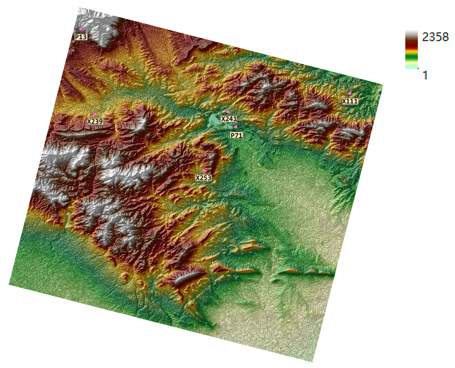
In the DSM generation experiment, we use the ZY-3 satellite images with a ground sampling distance of 3.5 m. Then, the generated epipolar images of Songshan are tested to obtain the corresponding DSM through the SGM-based stereo matching method and the Space Intersection method, and the result is shown in Figure 15. We compare the generated DSM with the DSM generated by other methods and the existing DSM to evaluate the accuracy of the DSM generated by our framework, based on the GCPs. We choose AW3D30 DSM and DSM generated by ENVI as comparison data. Among them, AW3D30 (ALOS World 3D-30 m) is a DSM data set released by the Japan Aerospace Exploration Agency(JAXA), with a grid resolution of ~30 m. This DSM data set is obtained by using PRISM on the land observation satellite ALOS to image the same object using three cameras with different perspectives [34]. In addition, the other DSM for comparison is obtained through the photogrammetry extension module in ENVI-v5.6 [35]. The ENVI software uses the metadata information of the ZY-3 original image pair to generate DSM.

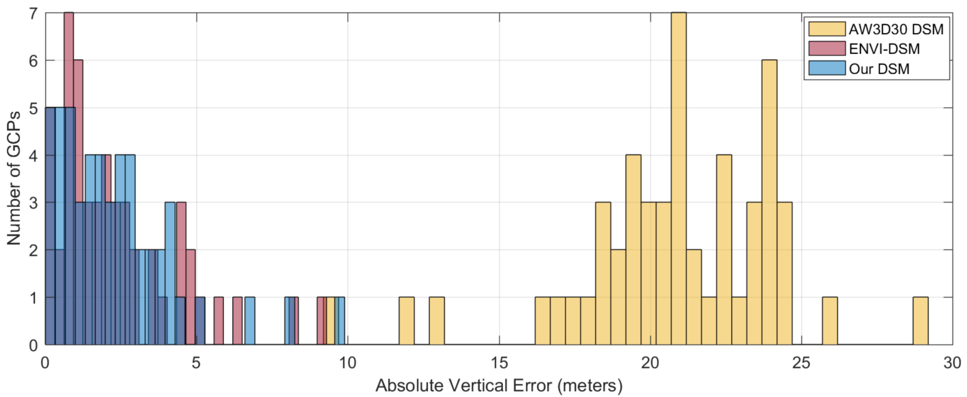
Comparing the generated DSM with GCPs, the absolute values of the difference between the elevation is mostly within 4 m, and the average absolute difference is 2.33 m. The histogram of the elevation accuracy is shown in Figure 16.

Table 7. The absolute vertical error of DSM. The GCP ID represents the number of the GCP. The average error is calculated from these 6 GCPs.

	Absolute Error (Meters)						Average Error
GCP ID	P13	X239	X241	P71	X253	X111	(Meters)
AW3D30 DSM	23.51	20.81	24.59	18.19	21.28	17.17	20.93
ENVI-DSM	0.70	1.09	3.68	1.18	1.28	2.99	1.82
Our DSM	0.51	0.81	1.59	1.81	1.28	0.83	1.14

lists the accuracy of DSM at the GCPs marked in Figure 15. Among them, the vertical precision of AW3D30 DSM in this area is ~20 m. Moreover, the vertical precision of ENVI-DSM and the generated DSM are both about 2 m. Therefore, the results show that the accuracy of the DSM we generated is greatly improved compared to AW3D30 DSM, and it can achieve higher accuracy than the DSM generated by ENVI. Therefore, the proposed framework can generate good quality epipolar images, which can be used to generate high accuracy DSM.

5. Conclusions

In this paper, we proposed a framework for generating epipolar images based on DEM constraints. DSM can be generated by stereo matching using the obtained approximate epipolar images. Through feature matching of the generated epipolar images, the epipolar images generated by our framework have higher precision and versatility, compared with the existing PTM method and the S2P method. The advantages of the proposed framework can be summarized as follows.

• The epipolar images generated by the proposed framework can better achieve the goal of restricting the search range of matching points from 2-D to 1-D for areas with large terrain undulations. Moreover, it is found that the matching points of the epipolar images have not only a small y-disparity, but also a small x-disparity. This shows that the search range of matching points can be further reduced, and the accuracy and speed of stereo matching will be improved, which is beneficial to ensure the efficiency of subsequent stereo matching work.
• This framework is also suitable for areas with small terrain undulations and can achieve ideal results. This can ensure that our framework can be used to generate epipolar images for the entire image with various scenarios. In addition to optical image pairs, this framework can be also applied to SAR-optical image pairs and SAR-SAR image pairs. This means that our framework has good versatility.
• The epipolar images generated by this framework can be applied to the generation of high-accuracy DSM. For optical image pairs, the average value of the elevation difference between the DSM generated by the proposed framework and the GCPs is no more than 3 m, which has good accuracy. That is, the proposed epipolar image generation framework can be used in subsequent DSM generation work.

Therefore, the epipolar image generation framework proposed in this paper is suitable for different terrains and various sensors, and a high-precision DSM can also be obtained. The influence of the size of image blocks on the accuracy of the generated DSM needs to be further verified as our framework divides the image into blocks. In addition, we also conducted experiments on the generation of DSM from SAR-SAR image pairs, but there are still some invalid and distorted values in the DSM. Therefore, we will investigate robust stereo matching methods for SAR images in our future works.

References

1. Wang, M.; Hu, F.; Li, J. Epipolar arrangement of satellite imagery by projection trajectory simplification. Photogramm. Rec. 2010, 25, 422–436. [Google Scholar] [CrossRef]
2. Morgan, M.F. Epipolar Resampling of Linear Array Scanner Scenes. PhD Thesis, University of Calgary, Calgary, AB, Canada, 2004. [Google Scholar]
3. Zhang, Z.; Zhou, Y. A New Approach to Arrange the Approximate Epipolar Lines for SPOT Images. J. Wuhan Tech. Univ. Surv. Mapp. 1989. Available online: https://en.cnki.com.cn/Article_en/CJFDTotal-WHCH198902002.htm (accessed on 20 September 2021).
4. Kim, T. A Study on the Epipolarity of Linear Pushbroom Images. Photogramm. Eng. Remote. Sens. 2000, 66, 961–966. [Google Scholar]
5. Oh, J.H.; Shin, S.W.; Kim, K.O. Direct Epipolar Image Generation From IKONOS Stereo Imagery Based On RPC and Parallel Projection Model. Korean J. Remote. Sens. 2006, 22, 451–456. [Google Scholar]
6. Wang, M.; Hu, F.; Li, J. Epipolar resampling of linear pushbroom satellite imagery by a new epipolarity model. Isprs J. Photogramm. Remote. Sens. 2011, 66, 347–355. [Google Scholar] [CrossRef]
7. Grodecki, J. IKONOS stereo feature extraction—RPC approach. In ASPRS Annual Conference St. Louis; 2001; Available online: https://www.researchgate.net/profile/Jacek-Grodecki/publication/228845277_IKONOS_stereo_feature_extraction-RPC_approach/links/5cacdc78458515cd2b0d25e2/IKONOS-stereo-feature-extraction-RPC-approach.pdf (accessed on 20 September 2021).
8. Oh, J.; Lee, W.H.; Toth, C.K.; Grejner-Brzezinska, D.A.; Lee, C. A Piecewise Approach to Epipolar Resampling of Pushbroom Satellite Images Based on RPC. Photogramm. Eng. Remote. Sens. 2010, 76, 1353–1363. [Google Scholar] [CrossRef]
9. Koh, J.W.; Yang, H.S. Unified piecewise epipolar resampling method for pushbroom satellite images. Eurasip J. Image Video Process. 2016, 2016, 11. [Google Scholar] [CrossRef] [Green Version]
10. Xiang, Y.; Wang, F.; You, H. OS-SIFT: A Robust SIFT-Like Algorithm for High-Resolution Optical-to-SAR Image Registration in Suburban Areas. IEEE Trans. Geosci. Remote. Sens. 2018, 56, 3078–3090. [Google Scholar] [CrossRef]
11. Bagheri, H.; Schmitt, M.; D’Angelo, P.; Zhu, X.X. A Framework for SAR-Optical Stereogrammetry over Urban Areas. ISPRS J. Photogramm. Remote. Sens. 2018, 146, 389–408. [Google Scholar] [CrossRef]
12. Qiu, C.; Schmitt, M.; Zhu, X.X. Towards automatic SAR-optical stereogrammetry over urban areas using very high resolution imagery. ISPRS J. Photogramm. Remote. Sens. 2018, 138, 218–231. [Google Scholar] [CrossRef] [PubMed]
13. Gutjahr, K.; Perko, R.; Raggam, H.; Schardt, M. The Epipolarity Constraint in Stereo-Radargrammetric DEM Generation. IEEE Trans. Geosci. Remote. Sens. 2014, 52, 5014–5022. [Google Scholar] [CrossRef]
14. Pan, H.B.; Guo, Z.; Chen, T. A general method of generating satellite epipolar images based on RPC model. In Proceedings of the 2011 IEEE International Geoscience and Remote Sensing Symposium, IGARSS 2011, Vancouver, BC, Canada, 24–29 July 2011. [Google Scholar]
15. Perko, R.; Gutjahr, K.; Krüger, M.; Raggam, H.; Schardt, M. DEM-based Epipolar Rectification for Optimized Radargrammetry. In Proceedings of the IEEE International Geoscience and Remote Sensing Symposium, Fort Worth, TX, USA, 23–28 July 2017. [Google Scholar]
16. Zhang, Z.; Yang, S.; Zhang, J.; Tao, K.E. Multi-Baseline Digital Close-Range Photogrammetry. Geospat. Inf. 2007, 5, 1–4. [Google Scholar]
17. Cho, W.; Schenk, T.; Madani, M. Resampling Digital Imagery to Epipolar Geometry. In Reports of the Department of Geodetic Science and Surveying; Ohio State University: Columbus, OH, USA, 1992. [Google Scholar]
18. Jia, K.X.; Xi, C.; Zheng, F.H. Study on the DSM Production and Application Based on Rapid Produced Three- Line Array Images of ZY- 3. Geomat. Spat. Inf. Technol. 2015, 38, 111–113. [Google Scholar]
19. Lemaître, M.; Verfaillie, G.; Jouhaud, F.; Lachiver, J.M.; Bataille, N. Selecting and scheduling observations of agile satellites. Aerosp. Sci. Technol. 2002, 6, 367–381. [Google Scholar] [CrossRef]
20. Meric, S.; Fayard, F.; Pottier, É. A Multiwindow Approach for Radargrammetric Improvements. IEEE Trans. Geosci. Remote. Sens. 2011, 49, 3803–3810. [Google Scholar] [CrossRef] [Green Version]
21. Hu, F.; Wang, M.; Li, D.; Xiao, M. Approximate Epipolar Rearrangement Algorithm of Satellite Stereo-imagery by Projection Trajectory. Geomat. Inf. Sci. Wuhan Univ. 2009, 34, 1431–1435. [Google Scholar]
22. Wilson, W.S.; Apel, J.R. The Principles of Photogrammetry, 2nd ed.; Wuhan University Press: Wuhan, China, 2009. [Google Scholar]
23. Teo, T.A.; Chen, L.C.; Liu, C.L.; Tung, Y.C.; Wu, W.Y. DEM-Aided Block Adjustment for Satellite Images With Weak Convergence Geometry. IEEE Trans. Geosci. Remote. Sens. 2010, 48, 1907–1918. [Google Scholar]
24. de Franchis, C.; Meinhardt-Llopis, E.; Michel, J.; Morel, J.M.; Facciolo, G. On stereo-rectification of pushbroom images. In Proceedings of the 2014 IEEE International Conference on Image Processing (ICIP), Paris, France, 27–30 October 2014; pp. 5447–5451. [Google Scholar] [CrossRef]
25. Xiang, Y.; Tao, R.; Wan, L.; Wang, F.; You, H. OS-PC: Combining Feature Representation and 3-D Phase Correlation for Subpixel Optical and SAR Image Registration. IEEE Trans. Geosci. Remote. Sens. 2020, 58, 6451–6466. [Google Scholar] [CrossRef]
26. Lowe, D. Distinctive image features from scaleinvariant keypoints. Int. J. Comput. Vis. 2004, 60, 91–110. [Google Scholar] [CrossRef]
27. Hartley, R.; Zisserman, A. Multiple View Geometry in Computer Vision, 2nd ed.; Cambridge University Press: Cambridge, UK, 2003. [Google Scholar] [CrossRef] [Green Version]
28. Hartley, R.I. In defense of the eight-point algorithm. IEEE Trans. Pattern Anal. Mach. Intell. 1997, 19, 580–593. [Google Scholar] [CrossRef] [Green Version]
29. Hartley, R.I. Theory and Practice of Projective Rectification. Int. J. Comput. Vis. 1999, 35, 115–127. [Google Scholar] [CrossRef]
30. Ozcanli, O.C.; Yi, D.; Mundy, J.L.; Webb, H.; Hammoud, R.; Tom, V. A comparison of stereo and multiview 3-D reconstruction using cross-sensor satellite imagery. In Proceedings of the Computer Vision & Pattern Recognition Workshops, Boston, MA, USA, 7–12 June 2015. [Google Scholar]
31. Beyer, R.A.; Oleg, A.; Scott, M.M. The Ames Stereo Pipeline: NASA’s Open Source Software for Deriving and Processing Terrain Data. Earth Space Sci. 2018, 5, 537–548. [Google Scholar] [CrossRef]
32. Hirschmüller, H. Stereo Processing by Semi-Global Matching and Mutual Information. IEEE Trans. Pattern Anal. Mach. Intell. 2008, 30, 328–341. [Google Scholar] [CrossRef] [PubMed]
33. Scharstein, D.; Szeliski, R.; Zabih, R. A taxonomy and evaluation of dense two-frame stereo correspondence algorithms. In Proceedings of the IEEE Workshop on Stereo and Multi-Baseline Vision (SMBV 2001), Kauai, HI, USA, 9–10 December 2001; pp. 131–140. [Google Scholar] [CrossRef]
34. Takaku, J.; Tadono, T.; Doutsu, M.; Ohgushi, F.; Kai, H. UPDATES OF ‘AW3D30’ ALOS GLOBAL DIGITAL SURFACE MODEL IN ANTARCTICA WITH OTHER OPEN ACCESS DATASETS. Int. Arch. Photogramm. Remote. Sens. Spat. Inf. Sci. 2021, 43, 401–408. [Google Scholar] [CrossRef]
35. ENVI-IDL Technology Hall. Extract DSM and Point Cloud Data Based on GF-7 Stereo Pair. 2021. Available online: http://blog.sina.com.cn/s/blog_764b1e9d010302tm.html (accessed on 15 April 2021).
Figure 1. A schematic diagram of the epipolar geometry relationship. O l and O r are respectively two cameras’ projection points. The projection of point P onto the left and right image are p l and p r . l r is the epipolar curve of point p l , and there has that p r must be on l r .
Remotesensing 13 04539 g001
Figure 2. Epipolar curves generated by PTM. The red and green dots represent conjugate point pairs. The red curves are the epipolar curves corresponding to the red dots. (a,b) GF-2 image pair. (c,d) GF-3 image pair.
Remotesensing 13 04539 g002
Figure 3. The fitting results of points on the projection trajectory of the GF-2 image pair. (a) Linear fitting residual. (b) Hyperbolic fitting residual.
Remotesensing 13 04539 g003
Figure 4. The fitting results of points on the projection trajectory of the GF-3 image pair. (a) The linear fitting residual. (b) The quartic polynomial fitting residual.
Remotesensing 13 04539 g004
Figure 5. The fitting results of points on the projection trajectory of the GF-2–GF-3 image pair. (a) The linear fitting residual. (b) The quadratic polynomial fitting residual.
Remotesensing 13 04539 g005
Figure 6. The fitting results of points on the projection trajectory of the GF-3–GF-2 image pair. (a) The linear fitting residual. (b) The high order polynomial fitting residual.
Remotesensing 13 04539 g006
Figure 7. (a) The linear fitting results of the epipolar curves in the left image corresponding to Points 1–6. These 6 points are selected from the same epipolar curve in the right image. (b) is the linear fitting results of the epipolar curves in the right image. Points 1–4 are the four randomly selected points in the left image.
Remotesensing 13 04539 g007
Figure 8. The flowchart of the proposed framework. The gray blocks indicate the processing of the entire image pairs, and the green blocks indicate the parallel processing of the image blocks.
Remotesensing 13 04539 g008
Figure 10. The epipolar images of two regions generated from ZY-3 images in Songshan. (a) The epipolar images generated by the S2P method. (b,c) The epipolar images generated by the PTM method and the proposed framework, respectively. ( x , y ) represents the coordinates of the corresponding point, where x is the horizontal coordinate and y is the vertical coordinate.
Remotesensing 13 04539 g010
Figure 11. The epipolar images of two regions generated from ZY-3 images in Tianshan. (a) The epipolar images generated by the S2P method. (b,c) The epipolar images generated by the PTM method and the proposed framework, respectively. ( x , y ) represents the coordinates of the corresponding point, where x is the horizontal coordinate and y is the vertical coordinate.
Remotesensing 13 04539 g011
Figure 12. The epipolar images generated from GeoEye images in Omaha. (a) The epipolar image pair generated by the S2P method. (b) The epipolar image pair generated by the proposed framework. ( x , y ) represents the coordinates of the corresponding point, where x is the horizontal coordinate and y is the vertical coordinate.
Remotesensing 13 04539 g012
Figure 13. The epipolar images generated from GF-3–GF-2 images in Songshan. (a) The epipolar image pair generated by the S2P method. (b) The epipolar image pair generated by the proposed framework. ( x , y ) represents the coordinates of the corresponding point, where x is the horizontal coordinate and y is the vertical coordinate.
Remotesensing 13 04539 g013
Figure 14. The epipolar images generated from GF-3–GF-3 images in Omaha. (a) The epipolar image pair generated by the S2P method. (b) The epipolar image pair generated by the proposed framework. ( x , y ) represents the coordinates of the corresponding point, where x is the horizontal coordinate and y is the vertical coordinate.
Remotesensing 13 04539 g014
Figure 15. The DSM generated by the proposed framework in Songshan. The dots represent the GCPs.
Remotesensing 13 04539 g015
Figure 16. The histogram of the elevation accuracy of the DSM relative to the GCPs.
Remotesensing 13 04539 g016