Article

Improving Estimates of Soil Salt Content by Using Two-Date Image Spectral Changes in Yinbei, China

1
State Key Laboratory of Remote Sensing Science, Faculty of Geographical Science, Beijing Normal University, Beijing 100875, China
2
Beijing Key Laboratory of Environmental Remote Sensing and Digital City, Faculty of Geographical Science, Beijing Normal University, Beijing 100875, China
3
NingXia Agriculture Technology Extension Service Centre, Yinchuan 750001, China
*
Author to whom correspondence should be addressed.
Remote Sens. 2021, 13(20), 4165; https://doi.org/10.3390/rs13204165
Submission received: 20 August 2021 / Revised: 29 September 2021 / Accepted: 14 October 2021 / Published: 18 October 2021
(This article belongs to the Section Biogeosciences Remote Sensing)

Abstract

:
Soil salt content (SSC) is normally featured with obvious spatiotemporal variations in arid and semi-arid regions. Space factors such as elevation, temperature, and spatial locations are usually used as input variables for a model to estimate the SSC. However, whether temporal patterns of salt-affected soils (identified as temporal spectral patterns) can indicate the SSC level and be applied as a covariate in a model to estimate the SSC remains unclear. Hence, temporal changes in soil spectral patterns need to be characterized and explored as to their use as an input variable to improve SSC estimates. In this study, a total of 54 field samples and a time-series of Sentinel-2 multispectral images taken at monthly intervals (from October 2017 to April 2018) were collected in the Yinbei area of western China. Then, two-date satellite images were used to quantify significant spectral changes over time using spectral change vector analysis, and four two-date-based index methods were used to characterize soil spectral changes. Lastly, the optimal two-date-based spectral indices and multispectral bands were used as input variables to build the estimation models using a random forest algorithm. Results showed that the two-date-based spectral index could be applied as an input variable to improve the accuracy of SSC estimation at a regional scale. Temporal changes in salt-induced spectral patterns can be indicated by the band difference in the wavelength range from 400 nm to 900 nm. Three two-date-based indices designated as D28a (i.e., the band difference between band 2 from an image acquired in April 2018 and band 8a from an image acquired in December 2017), D22, and D28 were the optimal parameters for characterizing salt-induced spectral changes, which were dominated by the total brightness, chloride, and sulfate accumulation of the soils. The model did not yield satisfactory estimation results (RPD = 1.49) when multispectral bands were used as the input variables. Multispectral bands coupled with two two-date-based indices (D22 and D28a) used as the input variables produced the best estimation result (R2 = 0.92, RPD = 3.27). Incorporating multispectral bands and two-date-based indices into the random forest model provides a remotely-sensed strategy that effectively supports the monitoring of soil salt content.

Graphical Abstract

1. Introduction

Soil salinization is an important land degradation and desertification process that usually occurs in arid and semi-arid environments and poses a threat to the ecological balance. Soils containing excessive salt adversely impact the material exchange in green plant cells, and reduce grain yield and agricultural productivity [1,2]. Soil salinization is a worldwide issue resulting from anthropogenic activities (e.g., excessive agricultural practices and flood irrigation) and global climate warming [3,4]. Soil productivity for 40 to 45% of the global land surface area has decreased due to different levels of salinity on salt-affected soil [5].
Prioritization should be given to solving this difficult environmental issue by early recognition, timely detection, and accurate processing of data for monitoring total soil salt content (SSC) with little spatial variability [6]. Remote sensing has the advantages of wide-area coverage and the ability to use upgraded available soil datasets. Remote sensing has recently become an effective method for identifying and monitoring SSC levels in salt-affected soils [7]. Hyperspectral satellite data has been shown to be a powerful tool for SSC monitoring as result of refined spectral recognition for soil attributes, but it has had limited use for large-scale, high-frequency SSC detection because the acquisition costs of hyperspectral data are expensive, and because available data do not widely cover the world [8]. Multispectral satellite imagery is also one of the important remote sensing data sources, due to its temporal regularity, the large quantity of image sources, and low acquisition costs, and, therefore, could be used for SSC estimation and salinity monitoring [9,10,11,12,13,14].
SSC can be estimated from satellite data by directly using the reflectivity in multispectral data, or by checking indirect links between environmental elements (e.g., climatic attributes, organisms, and topography parameters) and saline soil based on the scorpan model theory [15,16]. In the first case, the regional scale spatial distribution of salt status can be estimated by the reflectivity of multispectral bands and simultaneously collected field data using multivariate regression methods [17,18,19,20]. In this method, the limited number of multispectral bands and broad wavelengths have not provided sufficient detection of SSC features, and have restricted the improvement in estimation accuracy. Furthermore, some scholars [21,22,23,24,25] have argued that the regression models using multispectral data-derived indices and field-collected physicochemical data can improve the mapping of SSC levels at the regional scale. The result is that the application of multispectral data-derived indices (e.g., soil salinity indices and various ecological indices) is limited by the factors of climate elements, atmospheric conditions, land cover, and the spectral resolution of the different satellite platforms. In the second case, the accuracy of estimation modelling has increased and produced promising results for monitoring SSC status at a regional scale because input covariates have included additional environmental factors, such as topography, geology, temperature, and moisture [1,26,27,28,29,30,31]. This approach has great advantages in an area where the landscape has obvious variability. However, estimation accuracy would be decreased in large plain areas with a homogeneous environment.
As a matter of fact, apart from considering direct multispectral reflectance data and the indirect environmental influencing factors in the SSC model, the temporal spectral patterns are also a fundamental property of saline soils and are not sensitive to landscape patterns [16,32,33]. Specifically, salt accumulation in the soil is represented by a dense blocky formation or crust that is composed of white granular crystals on the surface layer. The combined crystal structure can increase the soil surface reflectance and produce significant spectral changes in the time of salt accumulation, such as changes in reflectance intensity and changes in the concave and convex pattern of spectral curves. These created spectral data show a close relationship with SSC level. Additionally, satellite images provide not only the geo-locations and spectral reflectance of the ground targets but also are able to provide temporal spectral information to illustrate the status of objects in study areas [34].
However, with regard to the temporal spectral information of salt-affected soils, whether it can indicate the SSC level, and whether it can be applied as an input variable in the model to estimate the SSC remains unclear. Hence, characterizing the temporal changes in soil spectral patterns and taking this as the input variable for improving estimates of SSC needs to be explored.
Characterizing the temporal changes in soil spectral patterns and modelling strategy selection are critical for improving SSC estimation. Two-date satellite images with significant spectral changes can contribute to providing temporal changes in spectral information that has a strong explanation capability regarding salt enrichment in the entire periods of salt accumulation. A two-date-based spectral index derived through the mathematical transformation of multidate satellite bands has been an effective tool for characterizing dynamic spectral information [35]. The two-date-based spectral index, including the band difference index, the ratio index, the normalized difference index, and the tangent of the angle formed by three bands, was constructed using paired multispectral satellite images to quantify the temporal changes in soil spectral information in this study. The difference index (D) and normalized difference index (ND) can be used to interpret spectral difference among two-date satellite bands because of the spectral intensity transitions of soil. Shape changes of spectral curves can be accessed by the tangent band index (tan). The ratio index (R) constructed by two-date satellite bands has the advantage of spectral feature integration and decreasing environmental impact in extracting soil spectral information. The generated spectral parameters reflect the different aspects of the physical and spectral change information of soil and can assist in the rapid recognition of salt-affected regions. However, an index that is powerful and strongly explains SSC levels still needs to be identified [21,36,37,38]. An ensemble machine learning approach, random forest algorithm (RF), has been widely used in solving complicated regression and classification problems, and is becoming popular for optimal spectral parameter identification. RF can assess the global importance scores of each variable via the increasing class of regression trees [39], and the selected variables can give more comprehensive details regarding SSC and provide perspectives and understanding of the mechanisms involved with spectral parameters. In the regression process, the selected spectral indices used as input variables have reduced model complexity and enable a more effective determination of SSC status [40].
In the Yinbei region of western China, bare soils are permanently exposed to the remote sensors during the dry season, which provides the optimal time window for multispectral satellite estimation of SSC. In this severe drought period, agricultural management (e.g., fertilizer application, irrigation, and crop cultivation) is temporarily suspended; biophysical activities (e.g., humus transformation and soil texture variation) also slow down. In contrast, soil salt actively moves to the surface and accumulates continuously under dry conditions. Based on the above premises, we assumed that SSC level could be indicated by the temporal changes in salt-affected soil spectral reflectance. Hence, this study’s objectives were to (1) estimate SSC using multispectral satellite images at a regional scale; (2) analyze spectral changes of two-date satellite images and build two-date-based spectral indices to characterize temporal changes in soil spectral reflectance; (3) evaluate the performance of the estimation model incorporating two-date-based spectral indices.

2. Materials and Methods
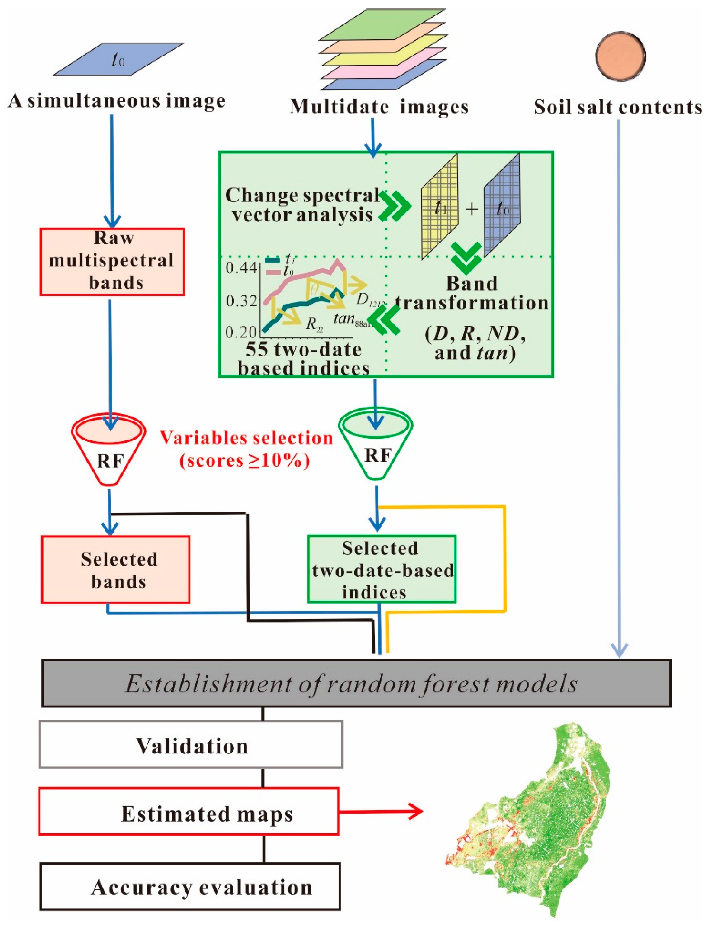
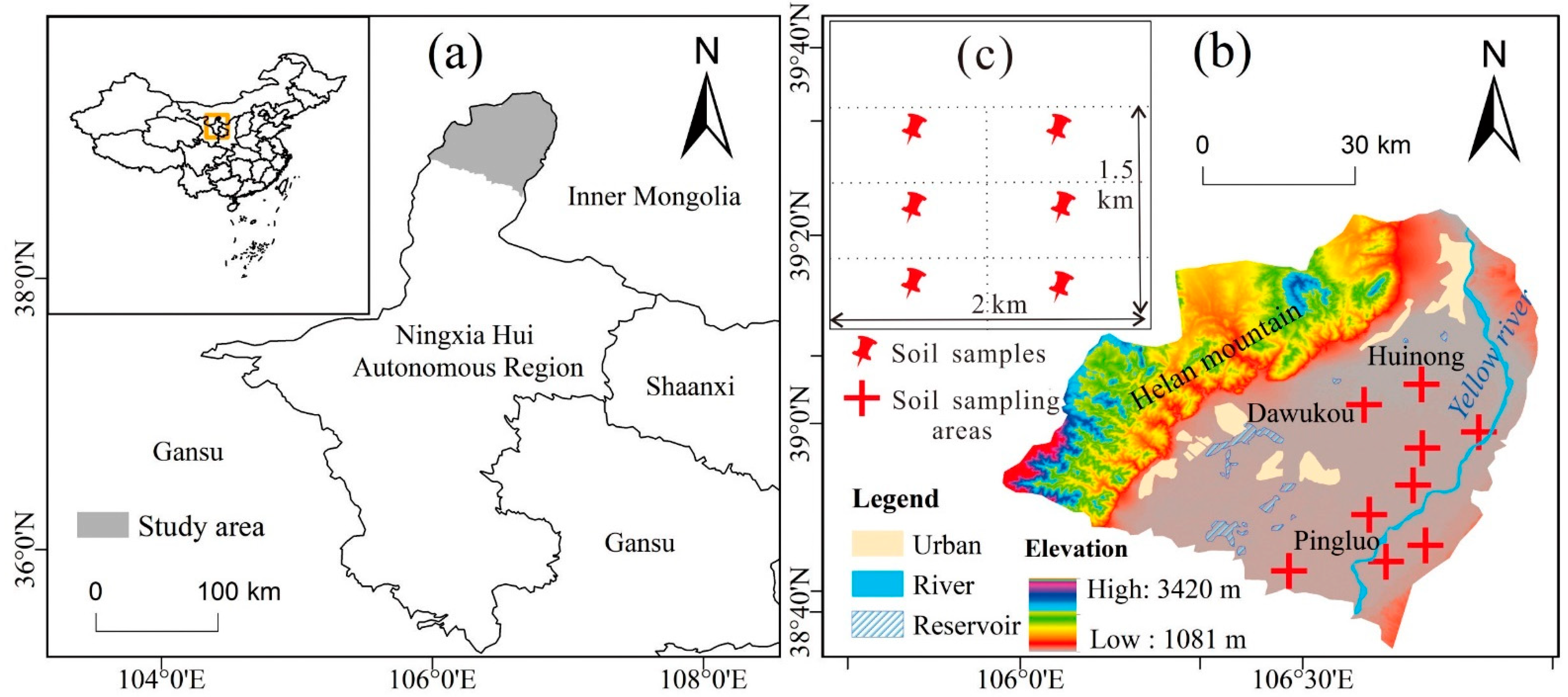
A flow chart of the analysis steps used in this study is shown in Figure 1. Acquisition and pre-processing of image data along with sampling and laboratory analysis were initially carried out. Secondly, spectral change analysis of multidate satellite images, construction of two-date-based indices, and determination of sensitive spectral parameters were completed. Lastly, RF models were determined and mapping results were obtained.

2.1. Study Area

The Yinbei region (38°35′56.4″ to 39°22′55.2″ N and 105°58′12.0″ to 106°55′8.4″ E) is located in the Northeast Ningxia Hui Autonomous Region of China, covers an area of 1000 km2, and has a population of 1.22 million (Figure 2a). An alluvial plain is located in the center of the study area, and the Helan Mountain Range is located in the western part of the Yinbei region. The Yellow River on the eastern boundary of the region provides a large amount of irrigation water for agricultural practices in the central plain. The study area has a temperate continental climate with a mean temperature of 9.69 °C, a mean annual precipitation of 187 mm, and an average annual evaporation of 1774 mm. The elevation ranges between 1081 m and 3420 m above sea level. The irrigation-silted soil and the alluvial soil are the major soil type in the Yinbei area. The common geological structures are faulted basins with aquifers characterized by loose rock pore water. The Yinbei area is a typical arid region of western China that suffers from soil salinization due to environmental elements including high evaporation rate, high groundwater table, and poor drainage. Irrigation infiltration accounts for 80% of the total groundwater recharge, the proportion of evaporated water is over 76% of the total groundwater discharge, and the rest of the water comes from groundwater runoff [41]. These factors have intensified soil degradation and produced an extremely fragile ecological environment [42].

2.2. Soil Sampling and Chemical Analysis

A total of 54 soil samples were collected from nine geographical areas (Figure 2b). Six samples were obtained within a 2 km by 1.5 km area at each site (Figure 2c). If soil could not be collected at the designated sites due to being covered by river and road, a close location was substituted for sample collection. All sampling sites had their actual locations recorded with a handheld global positioning system. Due to the active processes of salt accumulation, most soil salt accumulated on the surface layer of soil (0–5 cm); thereby, the representative samples were collected based on this depth. All samples were collected in April 2018 and then sealed in polyethylene bags for later laboratory analysis. In the laboratory, all non-soil materials were removed from the samples, including stones and weeds, and then the samples were dried and passed through a 1 mm sieve under normal conditions (25 °C). Total SSC was measured using the weighted method in which soil and water were mixed at a ratio of 1:5, the soluble salt in the soil was extracted by agitation of the solution and filtration, the filtrate extraction was evaporated until dry, and then the soil organic matter was removed using sodium hydroxide [27]. Then, the SSC at each sampling location was determined.

2.3. Time-Series Image Collection and Pre-Processing

The Sentinel-2 MultiSpectral Instrument (MSI) has a 10 m spatial resolution in four visible near-infrared spectroscopy bands, a 20 m spatial resolution in six red-edge and shortwave infrared (SWIR) bands, and a 60 m resolution for the coastal aerosol, water vapor, and cirrus band, the wavelength characteristics of bands are shown in Table 1 [43]. The revisiting frequency of Sentinel-2 MSI was up to 5 days. Monthly satellite images during the dry season (October 2017 to April 2018), including 21 cloudless (≤10%) Level-1 C sub-images, were acquired at no cost from https://glovis.usgs.gov/ (accessed on 23 November 2020). Three MSI sub-images within a month were mosaicked into one representative image. Atmospheric correction was performed with Sentinel Application Platform software (SNAP, version 6.0) equipped with the Sen2cor plugin (version 2.8) that can transform MSI-L1C products with top of atmosphere reflectance to the MSI-L2A product with bottom of atmosphere reflectance values [44]. Band 1, band 9, and band 10 at 60 m resolution were used for aerosol calibration, water vapor correction, and atmospheric feature detection, respectively, and, thus, were not included in the subsequent computation [11] The multispectral bands were all resampled at 10 m spatial resolution to reduce the adverse effects of mixed pixels. Additionally, the Yinbei region currently experiences periods of severe drought with low precipitation, and, therefore, the negative effect of soil moisture content on soil spectral reflectance is minimized.

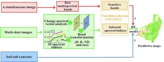
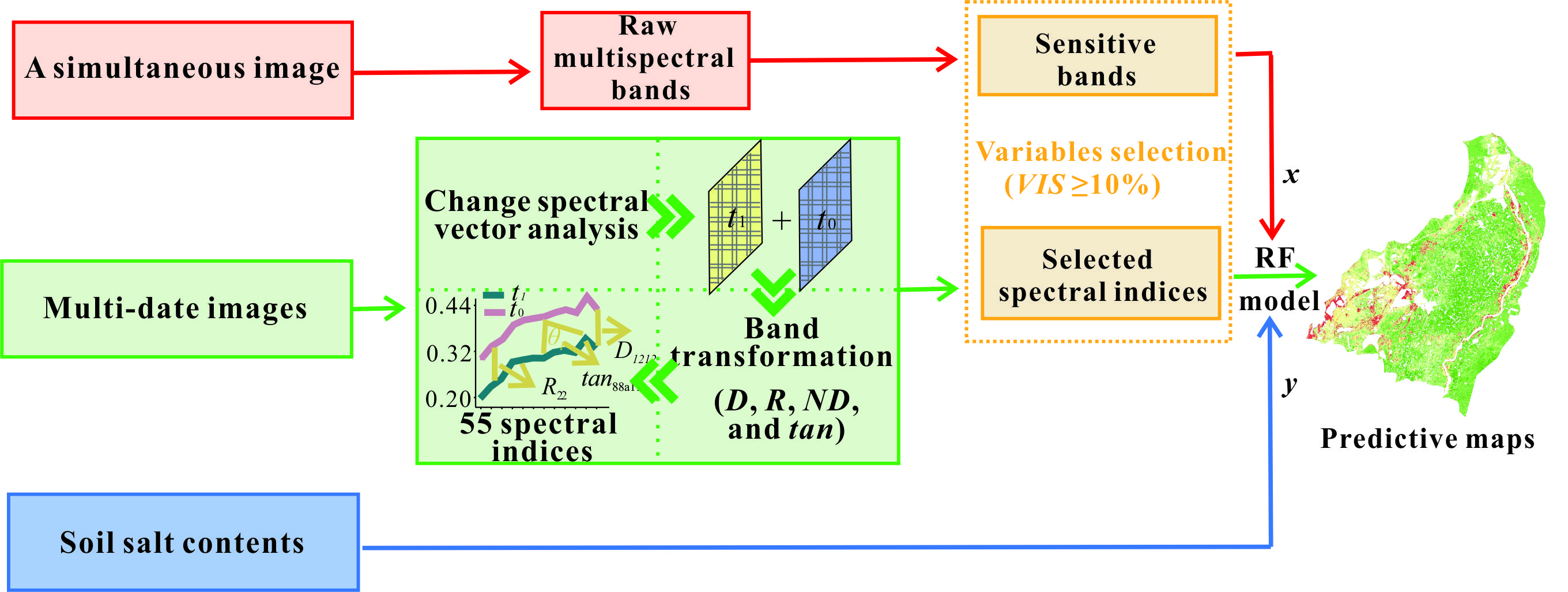
2.4. Modelling Strategies

The remote sensing estimation model used the different spectral parameters as the input variables, as represented in Table 2. Selecting sensitive spectral bands (i.e., the reflectance reflectivity of the multispectral band is an important covariate) and optimal two-date-based spectral indices were vital parts of this modelling strategy. In the first, the sensitive spectral bands were characterized with the high Variable Importance Scores (VIS), that were identified by the random forest algorithm; the two-date-based index was then constructed. The VIS are also a key parameter for highlighting the optimal two-date-based index. Lastly, the remote sensing estimation models were established by the regression relationships between the input variables and measured SSC data.

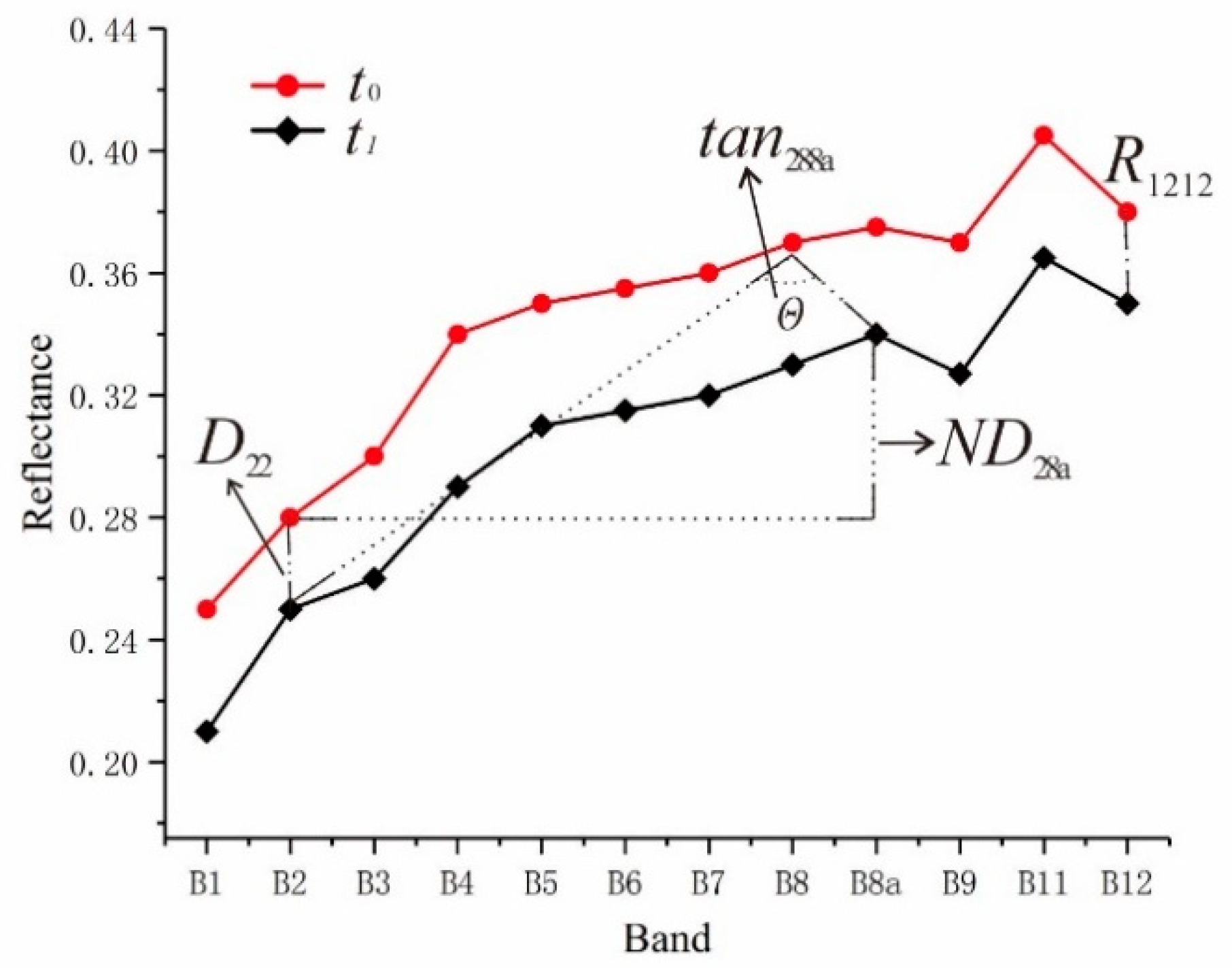
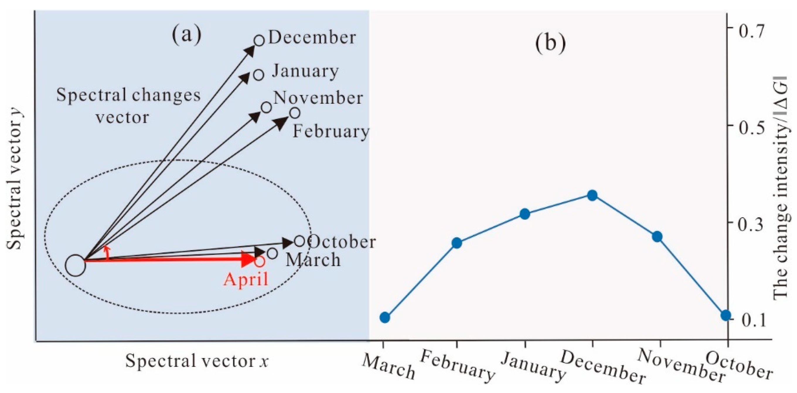
2.4.1. Detecting the Two-Date Images Spectral Changes

Increasing SSC increases soil spectral reflectance resulting from the high reflectivity of white salt granules. Two-date satellite images indicating obvious spectral changes are useful for revealing the salt increment on the surface soil layer in the entire period of salt accumulation [45,46]. Spectral change vector analysis is an effective method for evaluating the direction and magnitude of soil spectral reflectance changes that result from the changes in temporal salinization information, and facilitate the identification of the two-date images with significant spectral change information [47,48]. The computation process is given in Equation (1).
Δ G = 1 n i = 1 i = n ( g 1 h 1 ) 2 + ( g 2 h 2 ) 2 + + ( g i h j ) 2
where gi and hj represent the spectral vector of the image pixels of the temporal ith image and the temporal jth image, respectively, Δ G is the change intensity value. The calculation was conducted using MATLAB 2017b (MathWorks, Natick, MA, USA).
Soil spectral changes for the multidate satellite images included six two-date images (October 2017 and April 2018, November 2017 and April 2018, January 2018 and April 2018, February 2018 and April 2018, and March 2018 and April 2018), and were analyzed using spectral change vector analysis. The soil’s spectral reflectance changes in six two-date images can be judged by the change intensity value Δ G , with high values suggesting significant changes in soil spectral reflectance. The simultaneous temporal images captured in April 2018 were applied in concert with the field samples. After harvest, bare soils covered the Yinbei area beginning in October. Therefore, acquisition of the time-series images started in October 2017. Due to the availability of cloudless images for the Yinbei area, detection of soil spectral reflectance was conducted monthly (every 30 days). Additionally, the minimal period between images for capturing spectral reflectance changes due to soil salinization depended on the local area’s environmental condition (e.g., groundwater level, precipitation, and evaporation rate). In the study area, salt accumulation is a continuous process in long-term drought conditions; monthly satellite images can meet the requirement for detecting the temporal changes in soil spectral patterns.

2.4.2. Two-Date-Based Spectral Index Construction

The two-date-based spectral index is an effective tool that can help in acquiring temporal spectral patterns from the saline soil system [34,35]. As with the determination of the SSC sensitive bands from the simultaneous image and the optimal two-date images (t0 and t1), construction of the two-date-based index was based on the D, R, ND, and tan approaches. The equations for index construction are provided in Table 3. Figure 3 presents a case of two-date-based index establishment. The mathematical transformations of satellite bands were calculated with ENVI 5.3 IDL software (Exelis Visual Information Solutions, Boulder, CO, USA).

2.4.3. Random Forest Algorithm

In the random forest (RF) computation, the kth sub-datasets are randomly sampled from the original dataset, the β features are extracted from the m features of the sample, and the sub-dataset is modelled and optimized by the rest of the dataset [49]. Variable Importance Scores (VIS) depended on the proportion of the increment in the mean square error. In other words, model accuracy was assessed by the out-of-bag (OOB) error. A high VIS value means that the close relationship between spectral parameters and SSC, as well as the spectral parameters, have an obvious influence on the estimation result. VIS is expressed as follows
V I S ( X j ) = 1 n t r e e t ( e r r O O ˜ B t j e r r O O B t )
where t is the tree in the forest, OOBt is the linked portion not involved in bootstrap procedures for t establishment, errOOBt shows the error of the tth tree linked with the OOBt sample, and e r r O O ˜ B t j is the disturbed samplings of the Xj permuted value.
Input parameter selection and model estimation used the RF algorithm mentioned above and can be classified into three steps. In the first step, the collected spectral parameters (multispectral bands or spectral indices) were assessed for their ability to interpret SSC using the RF algorithm. Then, the same procedures were re-implemented to compute the VIS after discarding the 10% of parameters having the lowest VIS values until the number of spectral parameters in the remaining subset was less than 10 [50]. In order to ensure that there were a sufficient number of input variables and to save training time, a VIS threshold (10%) was set to identify the optimal spectral parameters [34]. Lastly, optimal spectral parameters were selected and participated in the subsequent calculations for model training and validation. The size of the input data (mtry) and the quantity of trees (ntree) were set to 7 and 1000, respectively, in the calculation. The VIS value and RF algorithm were processed via the R statistical computing package (R version 4.0.2, R Development Core Team, 2020). More details can be found in [51] and [49]. In order to test the applicability and the stability of the estimation model, the soil salt contents of the Yinbei region were estimated and mapped using the optimal constructed model.

2.5. Statistical Analysis

Based on the equations in Table 3, 55 two-date-based indices were generated based on the transformation of sensitive bands among two-date images, including 15 D indices, 15 R indices, 15 ND indices, and ten tan indices.
The coefficient of determination (R2) and the ratio of performance to deviation (RPD) were the statistical parameters for evaluating model accuracy and stability. The R2 value is the proportion of the target variable variation that is explained by the model, and the RPD value is the ratio of the standard deviation to the root mean square error. In general, the best model is characterized by high R2 and RPD values [52]. In the calibration and validation processes, a leave-one-out cross-validation was applied to assess model accuracy and stability, and the total dataset at each sampling involved the calibration and validation procession. Specifically, one sample was part of the calibration set after validation competition. According to the classification criterion from [53], RPD > 2 suggests that the model is more reliable with a higher predictive power, RPD values between 1.4 and 2 indicate that the model can generate moderately accurate outcomes, and RPD < 1.4 suggests that the model does not have adequate predictive capabilities.

3. Results

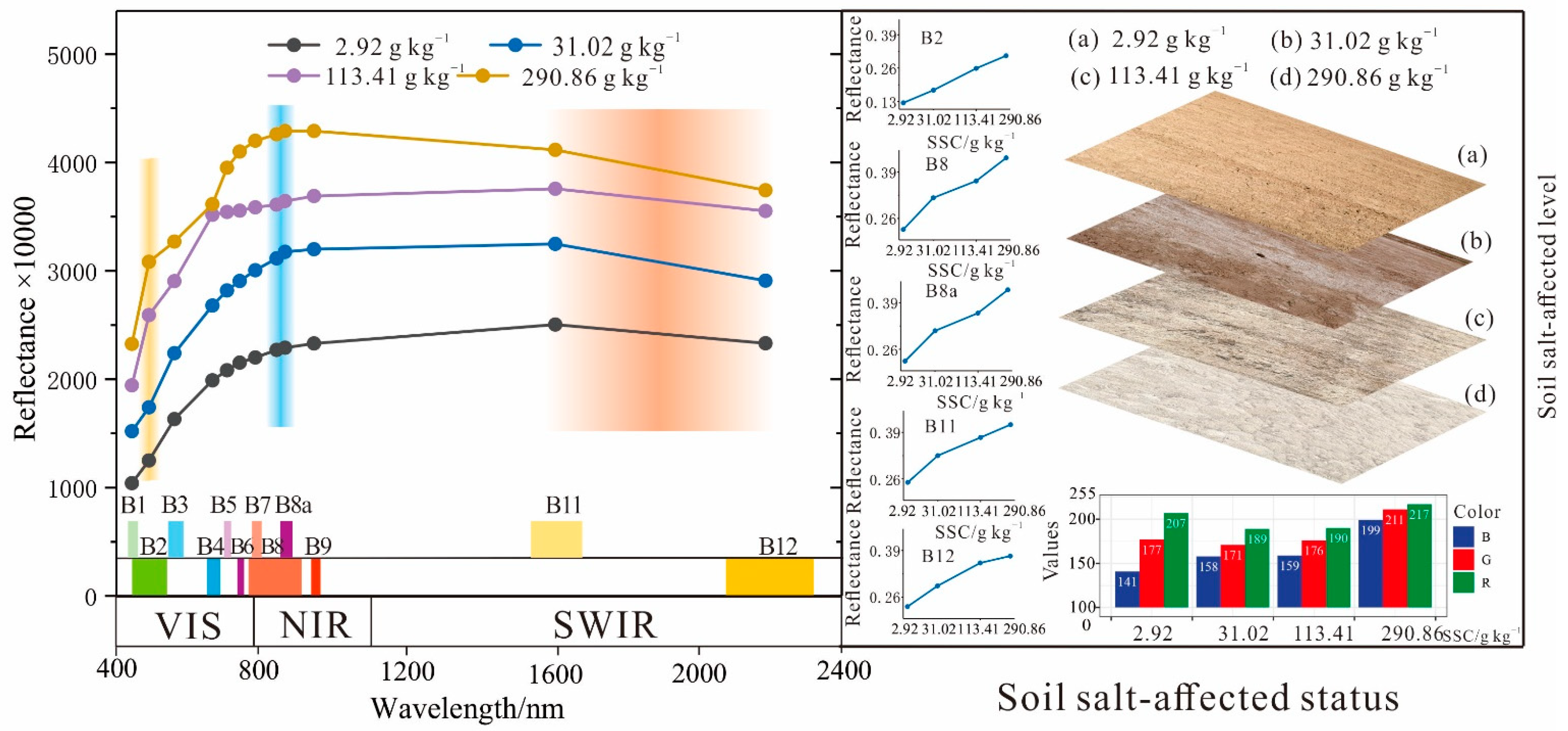
3.1. Characteristics of Soil Properties and Reflectance Spectra

The average value of SSC in the surface layer (0–5 cm) was 44.59 g kg1, with values of 2.92 g kg−1 to 290.86 g kg−1. The soil dataset had significant spatial variability in total salt contents, with the coefficient of variation for total salt content reaching 1.34, indicating a high variability level and the existence of representative values from the different soil type. The mean pH was 8.56, suggesting that the Yinbei area was moderately alkaline affected. The coefficient of skewness for SSC was 2.97. The distribution of elemental contents should possess a normal distribution, and a positive skew suggests that the outlier values arose from an exterior disturbance. According to the statistical analysis of SSC status, the sampling sites exhibited a high variability level of SSC, and a small portion of the hotspot area containing a high salt content represented an active process of soil salt accumulation.
The spectral reflectance visually showed the variation between samples with different levels of SSC (Figure 4). Reflectance intensity of the soil from sampled locations increased as the salt content rose from 2.92 g kg−1 to 290.86 g kg−1 in the MSI dataset. As shown in Figure 4, high salt content soils are more likely to exhibit a white salt crust on the topsoil and are characterized by higher spectral reflectance than soils with a lower soil salt content status. The correlation coefficients between satellite spectral data and measured SSC are displayed in Table 4. Reflectance intensity of all bands exhibited a positive correlation with SSC; band 2, band 8, band 8a, band 11, and band 12 were significantly correlated with SSC. Specifically, the reflectance of five bands changed significantly in soil with different salt-affected levels, showing higher reflectance for soils with SSC contents of 113.41 g kg−1 and 290.86 g kg−1 than for soil with SSC contents of 2.92 g kg−1 and 31.02 g kg−1. Soil reflectance increased as soil salt content increased across the entire spectrum, and the high spectral reflectance areas were located in the near-infrared wavelengths. In contrast, low spectral reflectance was observed in the visible spectra. The spectral curves shown in Figure 4 showed rapidly increasing reflectance in the visible regions as salt content increased. In general, the clearly different reflectance intensities of the spectral curves in the visible and near-infrared regions were helpful for distinguishing soils having different salt contents.
Changes in soil spectral reflectance showed a close relationship with SSC level. Dynamic hydrological processes drove salt accumulation in the topsoil of the Yinbei region, and created noticeable changes in the spectral reflectance of field soil. Four stages of the time of soil salt accumulation are illustrated in Figure 4. In the left panel, layer (a) shows a healthy status soil (low salt) after the crop is harvested and is characterized by grayness and lower reflectance. Following the salinization process, soil brightness increases (layer (b)). Layer (c) shows that the soil has been moderately affected by salt. Soil spectral reflectance at this stage began to represent salt mineral characteristics as a white salt crust begins to form. Lastly, salt signals significantly influence the soil spectral pattern of image pixels (layer (d)), showing the highest brightness and reflectivity among salt-affected soils. The spectral reflectance of the saline soil changes significantly in the time of active salinization processes (from layers (a) to (d)). Increasing soil surface brightness can enhance the soil’s reflecting power of electromagnetic energy and alter the reflectance intensities of the satellite spectral band. Additionally, the reflectance values in the range from 950 nm to 1650 nm were dominated by the stretch bending of the C-O and COO bonds; OH-Al banding form has a close relationship with the clay minerals and exhibited absorption features at 2200 nm; the mineral gypsum (CaSO4) is also an important component of saline soil, and spectral reflectance was observed at approximately 1730 nm. The white salt granules may be related with internal vibration in CaCO3 and the generated absorption bands around the wavelength of 2350 nm [31]. Thus, salt accumulation exhibited changes in spectral reflectance (reflectance intensity, changes in the concave and convex pattern of spectral curves). These spectral data show a close relationship with SSC and can be utilized as an SSC feature to provide the basis for improving the SSC estimation model.

3.2. Optimal Two-Date Satellite Images

The results of change vector analysis are shown in Figure 5 (Figure 5a represents the conceptual graph of changes of spectral vectors, and Figure 5b is the change intention values of different two-date images). The temporal changes in the spectral reflectance from time-series images (October 2017 to March 2018) to the simultaneous temporal image (April 2018, t0) have obvious differences, as shown by the change intensity value (‖ΔG‖) in the range from 0.04 to 0.34. The change intensity value between the December vector and the April vector reached 0.34, indicating that the spectral reflectance change for saline soils was highest. The January vector and the April vector also had a high change intensity value (0.31) that captured the marked changes in temporal spectral information related to soil salinization. The other two-date images did not show significant changes in the spectral reflectance of the soil as the change intensity value was lower than 0.30. In order to extract temporal changes in soil spectral information in the whole period of salt accumulation, the largest change intensity value was regarded as a standard for selecting the optimal two-date images. Therefore, the ideal times for acquiring two-date images (t0 and t1) were determined to be in April 2018 and December 2017, respectively.

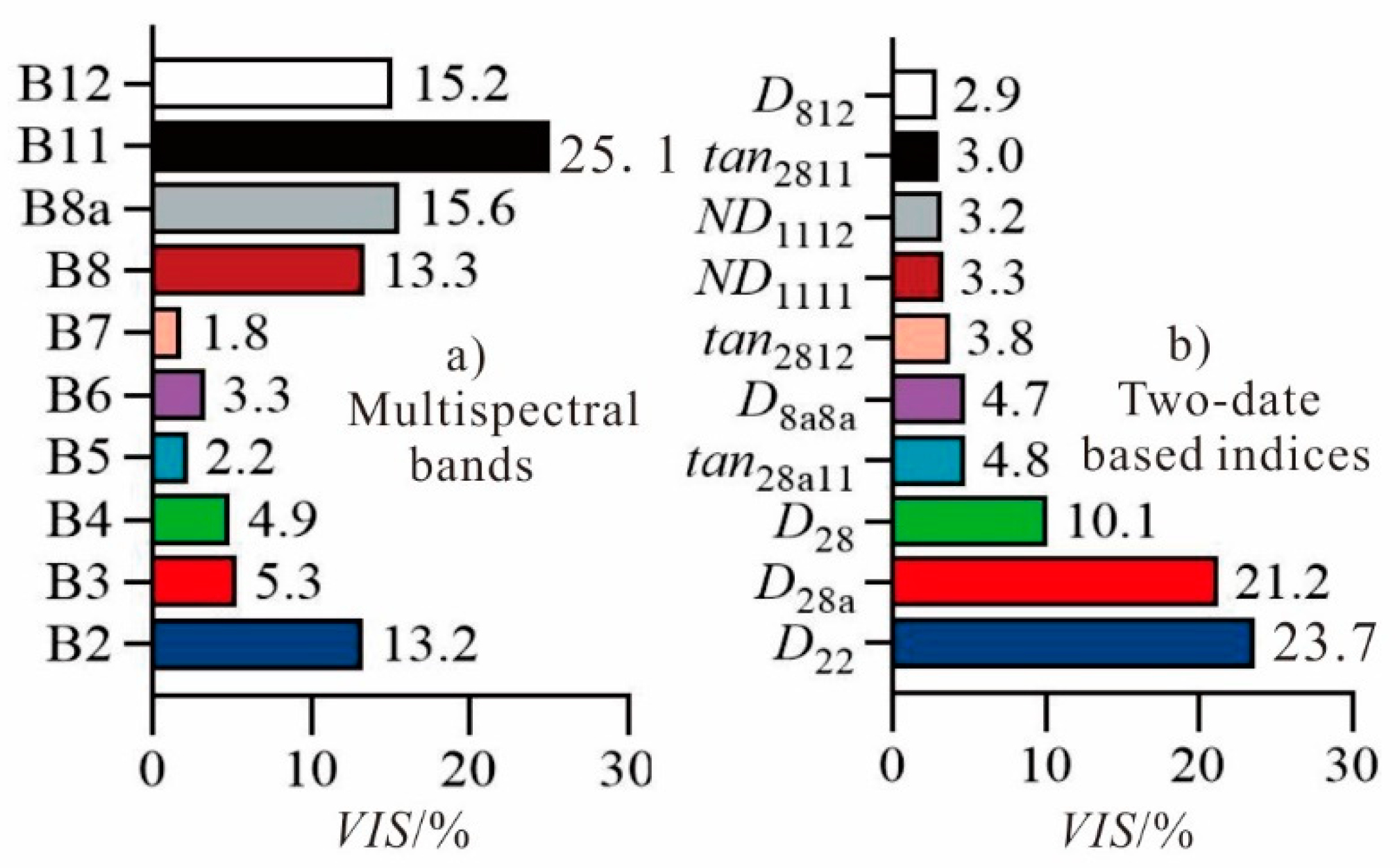
3.3. Sensitive Spectral Parameters

The RF importance scores of 10 single bands are shown in Figure 6a. B11 (shortwave infrared band) showed significant importance for soil salt. B2, B8, B8a, and B12 also have high VIS values (>10 %) and were selected as sensitive bands. The variable importance assessment approach was also implemented to select the optimal indices to quantify the salt-induced spectral changes. The calculation results are shown in Figure 6b. Obvious differences in VIS for the two-date-based indices existed in the four transformation methods. The most important indices (VIS > 10%) came from the band difference indices, such as D22, D28a, and D28. The ratio index scores did not rank in the top 10 and were lower than most of the index transformed methods calculated by the band difference, the band normalized difference, and the bands tangent. The band difference index was the most important method for highlighting salt-induced spectral changes. Therefore, five sensitive bands (B2, B8, B8a, B11, and B12) were selected, and the three optimal two-date-based indices (D22, D28a, and D28) were employed to characterize the temporal spectral patterns of salt-affected soils.

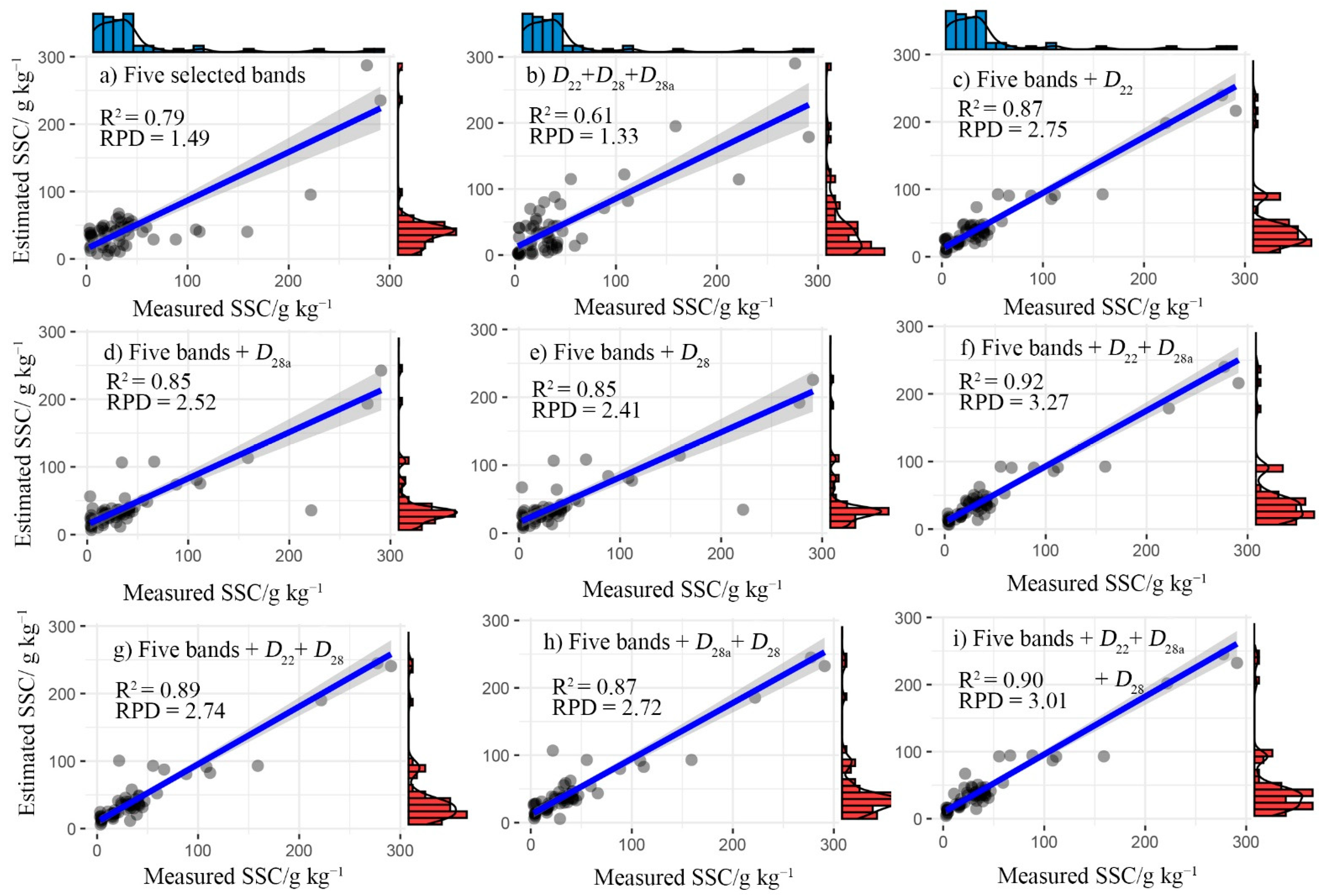
3.4. Performance Assessment of Prediction Models Built with Different Inputs

Results of the estimation models are shown in Figure 7. The models built with five sensitive bands (B2, B8, B8a, B11, and B12) and three optimal two-date-based indices (D22, D28a, and D28) had RPD values of 1.49 and 1.33, respectively, indicating that the models did not produce satisfactory estimation results. The RF model was constructed when five sensitive bands combined with an optimal two-date-based index (D22, D28a, and D28) as an input variable, as represented by the RPD values of 2.75, 2.52, and 2.41, respectively (Figure 7c–e). The optimal two-date-based indices used as a part of the input variable showed better accuracy than the five sensitive bands in the RF model. As shown in Figure 7f–i, different indices combinations were created to further analyze the capability of two-date-based indices to improve model accuracy. Figure 7c–h suggest that the model performance increased when the optimal two-date-based indices combination was used as an auxiliary input, as RPD values improved from the range of 2.41 to 2.75 to the range of 2.72 to 3.27. Five sensitive bands (B2, B8, B8a, B11, and B12) coupled with two optimal two-date-based indices (D22 and D28a) in the RF algorithm produced satisfactory estimation results (R2 = 0.92, RPD = 3.27) with the highest accuracy and stability.

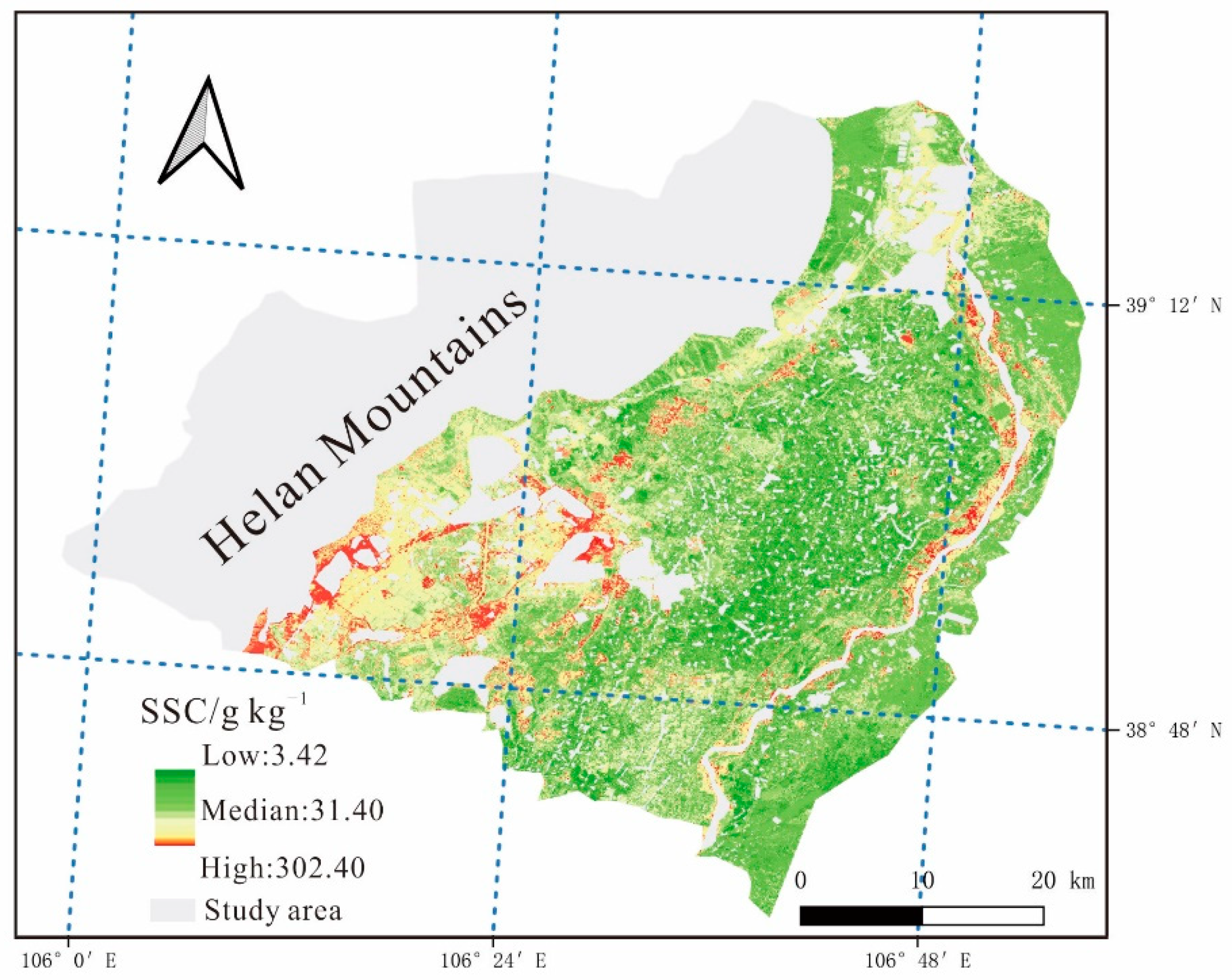
3.5. Map of Soil Salt Contents

The model was applied to each pixel of the MSI dataset in the study area, and the mapping result is presented in Figure 8. The results indicated that strong salt-affected areas were located in the southwest Yinbei area and on the two sides of the Yellow River, accounting for the areas of highest evaporation and lowest depth to groundwater. The growing demand for agricultural irrigation promotes salt water transportation and results in a considerable accumulation of soluble salt in surface soil. Figure 8 shows that SSC values in most of the Yinbei area were lower than 31.40 g kg−1 (72.06%). The results similarly identified the aforementioned descriptive statistics of this region. Additionally, high salt soils (31.40 g kg−1 < SSC ≤ 302.40 g kg−1) were observed to be scattered throughout the entire area shown in Figure 8. This can be explained by the fact that soil microtopography is shaped by agricultural irrigation that enables farmland to hold large amounts of irrigation water and leads to rising groundwater levels. Irrigation coupled with high evaporation results in a high level of SSC in the dry season.

4. Discussion

4.1. Characterizing Temporal Changes in Salt-Induced Spectral Information for Improving SSC Estimation

Choosing sensitive wavelength range was the key step for characterizing temporal changes in salt-induced spectral information. Several previous studies [11,18,54] have shown the close relationship between shortwave infrared bands and SSC, and regarded them as the key input parameters in SSC estimation. Nevertheless, the selected two-date-based indices did not involve the combination with B11. Bannari et al. [22], Jin et al. [55], and Shrestha [56] have suggested that band 11 is the critical indicator of soil salt. Areas with increased soil salinity levels normally exhibit increased coverage of the white salt crust, causing increased spectral reflectivity in almost every multispectral band (400–2500 nm) [11]. The different thicknesses of white salt crust in surface soils are mainly chloride and sulfate in the Yinbei area. Sodium chloride is normally observed as white granular crystals in the soil. In contrast, sodium sulfate belongs to the monoclinic crystal system and is observed as a dense blocky or shell-like structure on the soil surface [46,57,58,59]. The result is that high brightness with increasing reflectivity is produced in almost every spectral band of the soil. At the same time, the salt accumulation process in surface soils, soil alkalization, soil sodicity, and whitening of the surface color will also occur [60,61]. Bai et al. [17], Day [62], Lopez-Granados et al. [63], and Stoner et al. [64] have proven the significant relationships between SSC and soil alkalinity, with salt accumulated in soils that resulted from high pH and decreased soil organic matter. These changes influence soil color and the behavior of spectral features in the wavelength range from 350 nm to 1200 nm, and can be regarded as critical indicators of salt in field soil. The spectral bands responding to the salt-induced spectral changes in this study have also been observed at the susceptible regions from the visible near-infrared range (400–900 nm), similar to our findings. Therefore, the dynamic spectral information associated with SSC were especially sensitive to the band difference in the visible near-infrared range (400–900 nm) for the two-date satellite images.
The optimal estimation model can be constructed by the two-date-based indices with high VIS values. As shown in Figure 6, the VIS value of D22 was higher than the value of D28a of 10.55%; the estimation errors were 8.36% lower than for the model using D28a as an auxiliary input. Additionally, increasing the number of two-date-based indices used as input variables had a positive effect on the improvement in the model’s estimation accuracy, although a little estimation error of two-date models as a result of information redundancy between two-date-based indices will also arise. As shown in Figure 7c to Figure 7h, the accuracy of the two-date images model with seven independent variable inputs (five sensitive bands coupled with two two-date-based indices) was greater than that of the model with six independent variable inputs (five sensitive bands coupled with one two-date-based index). Nevertheless, the best estimation model was achieved when the auxiliary inputs were two two-date-based indices (D22 and D28a) rather than three two-date-based indices (D22, D28 and D28a). Collinear information existed between D28a and D28 because B8 and B8a contained common wavelength ranges and had similar responses for soils. Therefore, estimation errors arose for the model built with three two-date-based indices (D22, D28 and D28a).
The absence of a temporal spectral analysis of soil could restrict the performance improvement of an estimation model based on multispectral images. The results presented in this study provide a solution for analyzing the temporal changes in soil spectral patterns and increasing the explanatory ability of a multispectral remote sensing model for SSC, thereby promoting the ability to estimate SSC in an arid land.

4.2. Robustness of the Model Built with Two-Date-Based Indices

A satisfactory result was obtained using the two-date-based indices from the optimal two-date satellite images. The other two-date images during the bare soil period were employed to further examine the capability of the two-date image-based models. The optimal estimation results of the remaining five two-date image-based models are provided in Table 5. The two-date-based indices calculated from the remaining five two-date images also produced positive effects on the estimation accuracy of SSC modelling. The SSC model built with two-date images always showed better accuracy than the result derived from the single simultaneous image (Figure 7a). The two-date-based index’s introduction to the estimation model significantly improved accuracy. For example, the RPD values for the two-date model (January 2018 and April 2018) increased from 1.49 to 2.72. However, there were performance differences in the five two-date models. Specifically, the significance of salt-induced spectral changes was different between the six two-date images. The explanation capability of two-date-based indices for SSC was different, affecting the performance of two-date models. The best result and lowest accuracy of the two-date model were produced by the two-date images with obvious soil spectral changes (December 2017 and April 2018) and insignificant spectral changes (October 2017 and April 2018), respectively. Additionally, the multi-temporal images (three date images or more) could provide extra spectral covariates (i.e., multidate-based spectral indices) and could result in high degrees of information redundancy among spectral indices. Therefore, the effects on SSC modelling performance should be explored in the future.
The modelling strategies were also extended to the Operational Land Imager (OLI) dataset to verify the capability of the model built with the two-date-based indices. All bands in the OLI dataset exhibited a strong linear relationship with the MSI spectral reflectance on ground samples [54]. Two cloudless OLI images (December 2017 and April 2018) were acquired from https://glovis.usgs.gov/ (accessed on 25 November 2020) at no cost. Pre-processing procedures, including geometric correction, radiation correction, and atmospheric correction, were then performed [65]. The calculation results are shown in Table 5. RF using four sensitive bands (band 4, band 5, band 6, and band 7) as independent variables did not provide acceptable accuracy of SSC estimation (i.e., RPD value was lower than 1.40). The model’s accuracy was increased when the two-date-based indices (D55) were introduced as input variables, as the RPD value increased from 1.25 to 1.91. Results indicated that D55 was the only index with VIS value (37.79%) higher than 10%, and D55 was still the difference index combined by the bands in the near-infrared wavelengths of 400–900 nm. These findings verify the results from the MSI datasets that the salt-induced spectral change was more sensitive to different bands in the wavelength range of 400–900 nm among two-date images. The difference band index may be an effective method for quantifying the changes in temporal spectral patterns in the case of salt-affected soils. Analysis of the physical signals and temporal spectral patterns of objects in multispectral images boosts the SSC model’s accuracy and stability, and the generated accuracy was approximately equal to the accuracy of the models built with hyperspectral data reported in previous studies [66,67,68].
In general, temporal spectral patterns are a basic property of saline soils [33]. Extracted spectral change information (identified as the two-date-based spectral indices) can be an indicator of the SSC level, and, as such, we introduced them as input variables that increased the explanatory ability of estimation models for SSC. This modelling strategy has the benefits of simple operation and decreasing field work associated with investigating environmental covariates of salinization. This modelling strategy was also more appropriate for application in arid areas to which travel is inconvenient and climate is harsh. The temporal spectral patterns of salt-affected soil can also be used as a proxy with a new index design for monitoring SSC status.

4.3. Uncertainty Analysis

Salt accumulation in the surface soil and the associated temporal changes in the spectral patterns may not be linearly related. Apart from the aforementioned temporal salt-induced factors that can significantly affect the spectral reflectance of soils, environmental factors such as vegetation and moisture will also produce a certain influence on reflection intensity and the shapes of the spectral curve [69,70]. However, this part of the impact is minimized in the dry season of the Yinbei region of western China. The spectral changes in the period of salt accumulation constitute a complex synthetic signal that consists of soil substance signals (e.g., soil organic matter and soil irons), soil texture signals, and environmental signals [71]. As such, an analysis of the mechanisms causing salt-induced spectral changes will require further strict laboratory experiments.
The cross-validation method for remote sensing estimation of SSC may be optimistically biased. Although a leave-one-out cross-validation is an acceptable option for quality measures of the soil map, the autocorrelation existed in the soil dataset that can lead to overestimated estimation accuracy [72]. Designing an unbiased validation method and a design-based sampling strategy may be ideal for quality measures of remote sensing estimation [73]. However, that is beyond the range of our current study, and deserves to be studied in the next.
Mixed pixels of satellite images and small size datasets of field samples were the important factors contributing to modelling uncertainty. The small size dataset of field samples may increase data distribution variation and improve regression complications. Apart from ensuring the representation of each sampling collection, the RF model is a fully non-parametric method and did not assume linear linking in input variables, thereby promoting estimation efficiency such that a large sample size is not necessary [74,75]. Mixed pixels in the imagery dataset are an unavoidable problem [76]. Including the non-soil end-members leads to misidentification of spectral features and increased uncertainty. Soil sampling locations were designed to be at sites with pure soil pixels by assessing geographical consistency. Non-soil regions were excluded using the mask method to reduce the negative effect of outliers. The images mask is also implemented to decrease the interference of a foreign body with the spectrum, especially a few sandy soil areas on both sides of the Yellow River that had a spectral reflectance similar to that of saline soil. Therefore, ensuring that a soil’s reflectance is not contaminated by other targets is important for obtaining accurate results, and the decomposition of mixing pixels is still a topic to be studied in the future.

5. Conclusions

Characterizing temporal changes in soil spectral patterns as an input variable for an RF model can improve the remote sensing estimation of SSC (0–5 cm) at a regional scale. Results showed that band difference in the visible near-infrared range (400–900 nm) among two-date satellite bands was an effective method for characterizing dynamic spectral reflectance of the salt-affected soils. The total brightness, chloride, and sulfate accumulation of soils dominated optimal spectral parameters for characterizing salt-induced spectral changes. The sensitive multispectral bands included B2, B8, B8a, B11, and B12. B11 had the highest variable importance score. Sensitive bands as model inputs did not produce satisfactory estimation results (RPD = 1.49). Estimation accuracy for the model was increased when the two-date-based index was included as an input variable. The model built with the combination of five sensitive bands (B2, B8, B8a, B11, and B12) and two two-date-based indices (D22 and D28a) produced the best prediction result (R2 = 0.92, RPD = 3.27). Accurate and timely identification of changes in SSC on arid and semi-arid lands by use of the method we have described in this study can help producers and policy makers improve the understanding of the current salt-affected status so that they can implement effective measures for land restoration and soil reclamation.

Author Contributions

Writing and review, X.X., Y.C.; methodology, K.L.; software, Y.L.; validation, M.W.; pattern editing, S.W. All authors have read and agreed to the published version of the manuscript.

Funding

We thank the National Key R&D Program on monitoring, early warning and prevention of major natural disasters (Grant No. 2017YFC1502406) and Ningxia Agriculture and the Animal Husbandry Department East-West Cooperation Project “Study on Remote Sensing Monitoring of Agronomic Improvement of Saline-alkali Land in Yinbei Area” for financial support.

Institutional Review Board Statement

Not applicable.

Informed Consent Statement

Not applicable.

Data Availability Statement

The data presented in this research can be requested from the corresponding author or first author.

Acknowledgments

We thank Zhuo Chen and David Nielsen for English language support. We are also grateful to the anonymous reviewers for their constructive suggestions.

Conflicts of Interest

The authors declare no conflict of interest.

References

  1. Ma, L.; Ma, F.; Li, J.; Gu, Q.; Yang, S.; Wu, D.; Feng, J.; Ding, J. Characterizing and modeling regional-scale variations in soil salinity in the arid oasis of tarim basin, china. Geoderma 2017, 305, 1–11. [Google Scholar] [CrossRef]
  2. Metternicht, G.; Zinck, J. Remote sensing of soil salinity: Potentials and constraints. Remote Sens. Environ. 2003, 85, 1–20. [Google Scholar] [CrossRef]
  3. Teh, S.Y.; Koh, H.L. Climate change and soil salinization: Impact on agriculture, water and food security. Int. J. Agric. For. Plant 2016, 2, 1–9. [Google Scholar]
  4. Yang, X.; Yu, Y. Estimating soil salinity under various moisture conditions: An experimental study. IEEE Trans. Geosci. Electron. 2017, 55, 2525–2533. [Google Scholar] [CrossRef]
  5. White, R.P.; Tunstall, D.B.; Henninger, N. An Ecosystem Approach to Drylands: Building Support for New Development Policies; World Resources Institute: Washington, DC, USA, 2002. [Google Scholar]
  6. Nguyen, K.A.; Liou, Y.A.; Tran, H.P.; Hoang, P.P.; Nguyen, T.H. Soil salinity assessment by using near-infrared channel and vegetation soil salinity index derived from landsat 8 oli data: A case study in the tra vinh province, mekong delta, vietnam. Prog. Earth Planet Sci. 2020, 7, 1. [Google Scholar] [CrossRef] [Green Version]
  7. Chi, J.; Kim, H.C.; Lee, S.; Crawford, M.M. Deep learning based retrieval algorithm for arctic sea ice concentration from amsr2 passive microwave and modis optical data. Remote Sens. Environ. 2019, 231, 111204. [Google Scholar] [CrossRef]
  8. Vaudour, E.; Gomez, C.; Fouad, Y.; Lagacherie, P. Sentinel-2 image capacities to predict common topsoil properties of temperate and mediterranean agroecosystems. Remote Sens. Environ. 2019, 223, 21–33. [Google Scholar] [CrossRef]
  9. Bannari, A.; Al-Ali, Z.M. Assessing climate change impact on soil salinity dynamics between 1987–2017 in arid landscape using landsat tm, etm+ and oli data. Remote Sens. 2020, 12, 2794. [Google Scholar] [CrossRef]
  10. Fan, X.; Liu, Y.; Tao, J.; Weng, Y. Soil salinity retrieval from advanced multi-spectral sensor with partial least square regression. Remote Sens. 2015, 7, 488–511. [Google Scholar] [CrossRef] [Green Version]
  11. Wang, J.; Ding, J.; Yu, D.; Ma, X.; Zhang, Z.; Ge, X.; Teng, D.; Li, X.; Liang, J.; Lizaga, I.; et al. Capability of sentinel-2 msi data for monitoring and mapping of soil salinity in dry and wet seasons in the ebinur lake region, Xinjiang, China. Geoderma 2019, 353, 172–187. [Google Scholar] [CrossRef]
  12. Alexakis, D.; Daliakopoulos, I.; Panagea, I.; Tsanis, I. Assessing soil salinity using worldview-2 multispectral images in timpaki, crete, greece. Geocarto Int. 2018, 33, 321–338. [Google Scholar] [CrossRef]
  13. Chen, H.; Ma, Y.; Zhu, A.; Wang, Z.; Zhao, G.; Wei, Y. Soil salinity inversion based on differentiated fusion of satellite image and ground spectra. Int. J. Appl. Earth Obs. 2021, 101, 102360. [Google Scholar] [CrossRef]
  14. Hill, J.; Schütt, B. Mapping complex patterns of erosion and stability in dry mediterranean ecosystems. Remote Sens. Environ. 2000, 74, 557–569. [Google Scholar] [CrossRef]
  15. Muller, S.J.; Van Niekerk, A. Identification of worldview-2 spectral and spatial factors in detecting salt accumulation in cultivated fields. Geoderma 2016, 273, 1–11. [Google Scholar] [CrossRef]
  16. McBratney, A.B.; Santos, M.M.; Minasny, B. On digital soil mapping. Geoderma 2003, 117, 3–52. [Google Scholar] [CrossRef]
  17. Bai, L.; Wang, C.; Zang, S.; Zhang, Y.; Hao, Q.; Wu, Y. Remote sensing of soil alkalinity and salinity in the wuyu’er-shuangyang river basin, northeast china. Remote Sens. 2016, 8, 163. [Google Scholar] [CrossRef] [Green Version]
  18. Bannari, A.; El-Battay, A.; Bannari, R.; Rhinane, H. Sentinel-msi vnir and swir bands sensitivity analysis for soil salinity discrimination in an arid landscape. Remote Sens. 2018, 10, 855. [Google Scholar] [CrossRef] [Green Version]
  19. Davis, E.; Wang, C.; Dow, K. Comparing sentinel-2 msi and landsat 8 oli in soil salinity detection: A case study of agricultural lands in coastal north carolina. Int. J. Remote Sens. 2019, 40, 6134–6153. [Google Scholar] [CrossRef]
  20. Ekercin, S.; Ormeci, C. Estimating soil salinity using satellite remote sensing data and real-time field sampling. Environ. Eng. Sci. 2008, 25, 981–988. [Google Scholar] [CrossRef]
  21. Abbas, A.; Khan, S.; Hussain, N.; Hanjra, M.A.; Akbar, S. Characterizing soil salinity in irrigated agriculture using a remote sensing approach. Phys. Chem. Earth Parts A/B/C 2013, 55, 43–52. [Google Scholar] [CrossRef]
  22. Bannari, A.; El-Battay, A.; Hameid, N.; Tashtoush, F. Salt-affected soil mapping in an arid environment using semi-empirical model and landsat-oli data. Adv. Atmos. Remote Sens. 2017, 06, 260–291. [Google Scholar] [CrossRef] [Green Version]
  23. Gorji, T.; Sertel, E.; Tanik, A. Monitoring soil salinity via remote sensing technology under data scarce conditions: A case study from turkey. Ecol. Indic. 2017, 74, 384–391. [Google Scholar] [CrossRef]
  24. Sidike, A.; Zhao, S.; Wen, Y. Estimating soil salinity in pingluo county of china using quickbird data and soil reflectance spectra. Int. J. Appl. Earth Obs. 2014, 26, 156–175. [Google Scholar] [CrossRef]
  25. Wang, X.; Zhang, F.; Ding, J.; Kung, H.T.; Latif, A.; Johnson, V.C. Estimation of soil salt content (ssc) in the ebinur lake wetland national nature reserve (elwnnr), northwest china, based on a bootstrap-bp neural network model and optimal spectral indices. Sci. Total Environ. 2018, 615, 918–930. [Google Scholar] [CrossRef]
  26. Abdullah, A.Y.M.; Biswas, R.K.; Chowdhury, A.I.; Billah, S.M. Modeling soil salinity using direct and indirect measurement techniques: A comparative analysis. Environ. Dev. 2019, 29, 67–80. [Google Scholar] [CrossRef]
  27. Chi, Y.; Sun, J.; Liu, W.; Wang, J.; Zhao, M. Mapping coastal wetland soil salinity in different seasons using an improved comprehensive land surface factor system. Ecol. Indic. 2019, 107, 105517. [Google Scholar] [CrossRef]
  28. Guo, B.; Zang, W.; Zhang, R. Soil salizanation information in the yellow river delta based on feature surface models using landsat 8 oli data. IEEE Access 2020, 8, 94394–94403. [Google Scholar] [CrossRef]
  29. Han, L.; Liu, D.; Cheng, G.; Zhang, G.; Wang, L. Spatial distribution and genesis of salt on the saline playa at qehan lake, inner mongolia, china. Catena 2019, 177, 22–30. [Google Scholar] [CrossRef]
  30. Taghizadeh-Mehrjardi, R.; Minasny, B.; Sarmadian, F.; Malone, B. Digital mapping of soil salinity in ardakan region, central iran. Geoderma 2014, 213, 15–28. [Google Scholar] [CrossRef]
  31. Zovko, M.; Romić, D.; Colombo, C.; Di Iorio, E.; Romić, M.; Buttafuoco, G.; Castrignanò, A. A geostatistical vis-nir spectroscopy index to assess the incipient soil salinization in the neretva river valley, croatia. Geoderma 2018, 332, 60–72. [Google Scholar] [CrossRef]
  32. Rossel, R.V.; Fouad, Y.; Walter, C. Using a digital camera to measure soil organic carbon and iron contents. Biosyst. Eng. 2008, 100, 149–159. [Google Scholar] [CrossRef]
  33. Wadoux, A.M.C.; Minasny, B.; McBratney, A.B. Machine learning for digital soil mapping: Applications, challenges and suggested solutions. Earth-Sci. Rev. 2020, 210, 103359. [Google Scholar] [CrossRef]
  34. Boonprong, S.; Cao, C.; Chen, W.; Bao, S. Random forest variable importance spectral indices scheme for burnt forest recovery monitoring—Multilevel rf-vimp. Remote Sens. 2018, 10, 807. [Google Scholar] [CrossRef] [Green Version]
  35. Dou, X.; Wang, X.; Liu, H.; Zhang, X.; Meng, L.; Pan, Y.; Yu, Z.; Cui, Y. Prediction of soil organic matter using multi-temporal satellite images in the songnen plain, china. Geoderma 2019, 356, 113896. [Google Scholar] [CrossRef]
  36. Allbed, A.; Kumar, L.; Aldakheel, Y.Y. Assessing soil salinity using soil salinity and vegetation indices derived from ikonos high-spatial resolution imageries: Applications in a date palm dominated region. Geoderma 2014, 230–231, 1–8. [Google Scholar] [CrossRef]
  37. Peng, J.; Biswas, A.; Jiang, Q.; Zhao, R.; Hu, J.; Hu, B.; Shi, Z. Estimating soil salinity from remote sensing and terrain data in southern xinjiang province, china. Geoderma 2019, 337, 1309–1319. [Google Scholar] [CrossRef]
  38. Judkins, G.; Myint, S. Spatial variation of soil salinity in the mexicali valley, mexico: Application of a practical method for agricultural monitoring. Environ. Manag. 2012, 50, 478–489. [Google Scholar] [CrossRef]
  39. Gholizadeh, A.; Saberioon, M.; Ben-Dor, E.; Viscarra Rossel, R.A.; Boruvka, L. Modelling potentially toxic elements in forest soils with vis-nir spectra and learning algorithms. Environ. Pollut. 2020, 267, 115574. [Google Scholar] [CrossRef]
  40. Hong, Y.; Chen, S.; Chen, Y.; Linderman, M.; Mouazen, A.M.; Liu, Y.; Guo, L.; Yu, L.; Liu, Y.; Cheng, H. Comparing laboratory and airborne hyperspectral data for the estimation and mapping of topsoil organic carbon: Feature selection coupled with random forest. Soil Tillage Res. 2020, 199, 104589. [Google Scholar] [CrossRef]
  41. Yuan, F.; Lu, X.L.; Lu, F. Distribution characteristics of salty soil in northern yinchuan plain based on wet. South–North Water Transf. Water Sci. Technol. 2013, 11, 6. [Google Scholar]
  42. Wang, H.; Liu, W.J.; Wang, B. Protective cultivation technique model and its implementation benefit analysis in salt—Alkali area of upper and middle reaches of yellow river—Taking example for protective cultivation demonstration project in pingluo county of ningxia. Acta Agric. Jiangxi 2011, 23, 155–159. [Google Scholar]
  43. ESA. Sentinel-2 Spectral Response Functions (s2-srf)—Sentinel-2 Msi Document Library User Guides—Sentinel Online. Available online: https://earth.Esa.Int/web/sentinel/user-guides/sentinel-2-msi/document-library/-/asset_publisher/wk0tkajiisar/content/sentinel-2a-spectral-responses (accessed on 20 November 2020).
  44. Sibanda, M.; Mutanga, O.; Rouget, M. Examining the potential of sentinel-2 msi spectral resolution in quantifying above ground biomass across different fertilizer treatments. ISPRS J. Photogramm. 2015, 110, 55–65. [Google Scholar] [CrossRef]
  45. Yang, H.; Zhang, X.; Xu, M.; Shao, S.; Wang, X.; Liu, W.; Wu, D.; Ma, Y.; Bao, Y.; Zhang, X.; et al. Hyper-temporal remote sensing data in bare soil period and terrain attributes for digital soil mapping in the black soil regions of China. Catena 2020, 184, 104259. [Google Scholar] [CrossRef]
  46. Zhang, J.; Sun, Y.; Jia, K.; Gao, X.; Zhang, X. Spectral characteristics and salinization information prediction of different soil salt crusts. Trans. CSAE 2018, 49, 325–333. [Google Scholar]
  47. Singh, S.; Talwar, R. Response of fuzzy clustering on different threshold determination algorithms in spectral change vector analysis over western himalaya, india. J. Mt. Sci. 2017, 14, 1391–1404. [Google Scholar] [CrossRef]
  48. Chen, J.; Gong, P.; He, C.; Pu, R.; Shi, P. Land-use/land-cover change detection using improved change-vector analysis. Photogramm. Eng. Remote Sens. 2003, 69, 369–379. [Google Scholar] [CrossRef] [Green Version]
  49. Breiman, L. Random forests. Mach. Learn. 2001, 45, 5–32. [Google Scholar] [CrossRef] [Green Version]
  50. Archer, K.J.; Kimes, R.V. Empirical characterization of random forest variable importance measures. Comput. Stat. Data Anal. 2008, 52, 2249–2260. [Google Scholar] [CrossRef]
  51. Grömping, U. Variable importance assessment in regression: Linear regression versus random forest. Am. Stat. 2009, 63, 308–319. [Google Scholar] [CrossRef]
  52. Xu, Y.; Wang, X.; Bai, J.; Wang, D.; Wang, W.; Guan, Y. Estimating the spatial distribution of soil total nitrogen and available potassium in coastal wetland soils in the yellow river delta by incorporating multi-source data. Ecol. Indic. 2020, 111, 106002. [Google Scholar] [CrossRef]
  53. Andrade, R.; Faria, W.M.; Silva, S.H.G.; Chakraborty, S.; Weindorf, D.C.; Mesquita, L.F.; Guilherme, L.R.G.; Curi, N. Prediction of soil fertility via portable x-ray fluorescence (pxrf) spectrometry and soil texture in the brazilian coastal plains. Geoderma 2020, 357, 113960. [Google Scholar] [CrossRef]
  54. Bannari, A.; Hameid Mohamed Musa, N.; Abuelgasim, A.; El-Battay, A. Sentinel-msi and landsat-oli data quality characterization for high temporal frequency monitoring of soil salinity dynamic in an arid landscape. IEEE J. STARS 2020, 13, 2434–2450. [Google Scholar] [CrossRef]
  55. Jin, P.; Li, P.; Wang, Q.; Pu, Z. Developing and applying novel spectral feature parameters for classifying soil salt types in arid land. Ecol. Indic. 2015, 54, 116–123. [Google Scholar] [CrossRef]
  56. Shrestha, R. Relating soil electrical conductivity to remote sensing and other soil properties for assessing soil salinity in northeast thailand. Land Degrad. Dev. 2006, 17, 677–689. [Google Scholar] [CrossRef]
  57. Çelik, M.Y.; Aygün, A. The effect of salt crystallization on degradation of volcanic building stones by sodium sulfates and sodium chlorides. Bull. Eng. Geol. Environ. 2019, 78, 3509–3529. [Google Scholar] [CrossRef]
  58. Kamburov, S.; Schmidt, H.; Voigt, W.; Balarew, C. Similarities and peculiarities between the crystal structures of the hydrates of sodium sulfate and selenate. Acta Crystallogr. Sect. B Struct. Sci. Cryst. Eng. Mater. 2014, 70, 714–722. [Google Scholar] [CrossRef]
  59. Zhang, F.; Xiong, H.; Ding, J.; Xia, Q. Characteristics of laboratory-field measured spectra responding to alkalinized soil and conversion. Trans. CSAE 2012, 28, 101–107. [Google Scholar]
  60. Liu, F.R.; Li, L.R. Current status of cultivated soil salinization in yinbei irrigation district of ningxia and its prevention countermeasures. Ningxia J. Agric. For. Sci. Technol. 2008, 2, 63–64. [Google Scholar]
  61. Panda, B.C. Remote Sensing: Principle and Application; Viva Books Pvt Ltd.: New Delhi, India, 2005. [Google Scholar]
  62. Day, A.D.; Ludeke, K.L. Soil alkalinity. In Plant Nutrients in Desert Environments; Springer: Berlin/Heidelberg, Germany, 1993; pp. 35–37. [Google Scholar]
  63. López-Granados, F.; Jurado-Expósito, M.; Peña-Barragán, J.M.; García-Torres, L. Using geostatistical and remote sensing approaches for mapping soil properties. Eur. J. Agron. 2005, 23, 279–289. [Google Scholar] [CrossRef]
  64. Stoner, E.R. Physicochemical, Site, and Bidirectional Reflectance Factor Characteristics of Uniformly-Moist Soils; Purdue University: West Lafayette, IN, USA, 1979. [Google Scholar]
  65. Masoud, A.A.; Koike, K.; Atwia, M.G.; El-Horiny, M.M.; Gemail, K.S. Mapping soil salinity using spectral mixture analysis of landsat 8 oli images to identify factors influencing salinization in an arid region. Int. J. Appl. Earth Obs. 2019, 83, 101944. [Google Scholar] [CrossRef]
  66. Kahaer, Y.; Tashpolat, N.; Shi, Q.; Liu, S. Possibility of zhuhai-1 hyperspectral imagery for monitoring salinized soil moisture content using fractional order differentially optimized spectral indices. Water 2020, 12, 3360. [Google Scholar] [CrossRef]
  67. Wang, L.; Zhang, B.; Shen, Q.; Yao, Y.; Zhang, S.; Wei, H.; Yao, R.; Zhang, Y. Estimation of soil salt and ion contents based on hyperspectral remote sensing data: A case study of baidunzi basin, China. Water 2021, 13, 559. [Google Scholar] [CrossRef]
  68. Weng, Y.; Gong, P.; Zhu, Z. Soil salt content estimation in the yellow river delta with satellite hyperspectral data. Can. J. Remote Sens. 2008, 34, 259–270. [Google Scholar]
  69. Ji, W.; Li, S.; Chen, S.; Shi, Z.; Rossel, R.A.V.; Mouazen, A.M. Prediction of soil attributes using the chinese soil spectral library and standardized spectra recorded at field conditions. Soil Till. Res. 2016, 155, 492–500. [Google Scholar] [CrossRef]
  70. Guo, L.; Zhang, H.; Shi, T.; Chen, Y.; Jiang, Q.; Linderman, M. Prediction of soil organic carbon stock by laboratory spectral data and airborne hyperspectral images. Geoderma 2019, 337, 32–41. [Google Scholar] [CrossRef]
  71. Pessoa, L.G.M.; Freire, M.B.G.D.S.; Wilcox, B.P.; Green, C.H.M.; De Araújo, R.J.T.; De Araújo Filho, J.C. Spectral reflectance characteristics of soils in northeastern brazil as influenced by salinity levels. Environ. Monit. Assess. 2016, 188, 1–11. [Google Scholar] [CrossRef] [PubMed]
  72. Brus, D.; Kempen, B.; Heuvelink, G. Sampling for validation of digital soil maps. Eur. J. Soil Sci. 2011, 62, 394–407. [Google Scholar] [CrossRef]
  73. Wadoux, A.M.J.C.; Brus, D.J.; Heuvelink, G.B.M. Sampling design optimization for soil mapping with random forest. Geoderma 2019, 355, 113913. [Google Scholar] [CrossRef]
  74. Grimm, R.; Behrens, T.; Märker, M.; Elsenbeer, H. Soil organic carbon concentrations and stocks on barro colorado island—Digital soil mapping using random forests analysis. Geoderma 2008, 146, 102–113. [Google Scholar] [CrossRef]
  75. Xu, L.; Saatchi, S.S.; Yang, Y.; Yu, Y.; White, L. Performance of non-parametric algorithms for spatial mapping of tropical forest structure. Carbon Bal. Manag. 2016, 11, 1–14. [Google Scholar] [CrossRef] [Green Version]
  76. Liu, Y.; Zhang, F.; Wang, C.; Wu, S.; Liu, J.; Xu, A.; Pan, K.; Pan, X. Estimating the soil salinity over partially vegetated surfaces from multispectral remote sensing image using non-negative matrix factorization. Geoderma 2019, 354, 113887. [Google Scholar] [CrossRef]
Figure 1. Flowchart of the process used for estimating soil salt content in the Yinbei region, China. RF: random forest; t0 and t1 represent optimal two-date satellite images; D: band difference; R: band ratio; ND: band normalized difference; tan: the tangent of the angle formed by three bands.
Remotesensing 13 04165 g001
Figure 2. Geographical location of sampling sites in the Yinbei region, China: (a) location of Yinbei study area within China; (b) locations of sampling area; (c) samples sites at each sampling area.
Remotesensing 13 04165 g002
Figure 3. Illustration of two-date-based index construction using two-date images (t0 and t1) in the Yinbei region, China. Note: D22 is the difference between B2 from image t0 and B2 from image t1. R1212 is the ratio in B12 between t0 and t1; ND28a is the normalized difference index of band 2 and band 8a. tan288a represents the tangent of the angle of three bands (B2, B8, and B8a) of images t0 and t1, where B8 comes from image t0 and B8a and B2 come from image t1.
Remotesensing 13 04165 g003
Figure 4. Spectral bands from the MSI datasets and geographic status of soils with different salt-affected classes in the Yinbei region, China: VIS, NIR, and SWIR represent the spectral wavelength of the visible, near-infrared, and shortwave infrared. The right panel indicates the spectral curves of soils with different salt contents and the sensitive wavelength ranges of soil salt contents. Geographic features of different salt-affected soil and the resulting specifications of five typical bands and colors are displayed in the left panel.
Remotesensing 13 04165 g004
Figure 5. Change vector analysis for the soil spectral reflectance from the simultaneous image (April 2018) to time-series images (October 2017 to March 2018) in the Yinbei region, China: (a) conceptual graph of temporal changes in spectral vectors; (b) the change intensity values of different two-date images.
Remotesensing 13 04165 g005
Figure 6. Spectral parameter selection results (a): multispectral bands and (b): two-date-based indices in the Yinbei region, China; VIS is the variable importance score; Dij represents the band difference between the band i from the image acquired in April 2018 and band i from image t1 acquired in December 2017; NDij is the normalized difference index of band i and band j; tanimj is the tangent of the angle calculated by three bands (band i, band j, and band m).
Remotesensing 13 04165 g006
Figure 7. Scatter plot of measured versus estimated soil salt content (SSC) using RF models built with the different input variables: (a) five sensitive bands; (b) D22, D28a, and D28; (c) five sensitive bands and D22; (d) five sensitive bands and D28a; (e) five sensitive bands and D28; (f) five sensitive bands, D22, and D28a; (g) five sensitive bands, D22, and D28; (h) five sensitive bands, D28a, and D28; (i) five sensitive bands, D22, D28a, and D28. R2: coefficient of determination; RPD: ratio of performance to deviation; Dij means the band difference among two-date satellite bands.
Remotesensing 13 04165 g007
Figure 8. Map of soil salt contents (SSC) of the Yinbei region, China.
Remotesensing 13 04165 g008
Table 1. Spectral bands of the MSI dataset.
Band AcronymB1B2B3B4B5B6B7B8B8aB9B10B11B12
Band centre/nm443490560665705740775842865940137516102190
Band width/nm2065353015152011520203090180
Table 2. List of the input variables and its sources for the random forest estimation model.
NumberInput VariablesData Sources
1Sensitive spectral bandsThe simultaneous image
2Optimal two-date-based indicesThe two-date images
3Sensitive spectral bands and optimal two-date-based spectral indicesThe two-date images
Table 3. Two-date-based spectral index construction using the two-date images (t0 and t1) in the Yinbei region, China.
Index AbbreviationCalculation ImageEquation
Dijt0, t1Bi − Bj
Rijt0, t1Bi/Bj
NDijt0, t1(Bi − Bj)/(Bi + Bj)
tanimjt0, t1(kimkmj)/(1 + kim·kmj)
Note: Bi is the ith sensitive band in the multispectral image (t0), Bj is the jth sensitive band in the image (t1), Dij represents the difference between Bi and Bj, Rij indicates the ratio of Bi and Bj, NDij is the normalized difference index of band i and band j; tanimj is the tangent of the angle calculated by three bands (ith band, mth band, and jth band), where the mth band comes from (t0) and the other bands are derived from (t1). kim is computed by the slope of the linking line between ith and mth band. kmj is also calculated by the slope of the linking line between mth and jth band.
Table 4. Pearson correlation coefficient for the satellite spectral data and measured soil salt contents (SSC).
Band AcronymB2B3B4B5B6B7B8B8aB11B12
SSC0.49 *0.460.470.470.480.48 *0.49 **0.49 **0.50 **0.41 *
* represents the correlation that is significant at 0.05 level; ** represents the correlation that is significant at 0.01 level.
Table 5. Performance comparison of estimation models constructed using two-date satellite data in the Yinbei region, China.
NumberSatellite PlatformCapture Time of Two-Date ImagesOptimal InputsR2RPD
1Sentinel-2_MSI dataOctober 2017 and April 2018B2, B8, B8a, B11, B12, and ND8a8a0.791.45
2November 2017 and April 2018B2, B8, B8a, B11, B12, and D220.852.43
3January 2018 and April 2018B2, B8, B8a, B11, B12,
D22, and D28a
0.872.72
4February 2018 and April 2018B2, B8, B8a, B11, B12,
D22, and D28a
0.821.93
5March 2018 and April 2018B2, B8, B8a, B11, B12,
and tan28a11
0.821.82
6Landsat-8_OLI dataApril 2018B4, B5, B6, and B70.721.25
7December 2017 and April 2018B4, B5, B6, B7, and D550.811.91
Note: R2 is the coefficient of determination; RPD is the ratio of performance to deviation.
Publisher’s Note: MDPI stays neutral with regard to jurisdictional claims in published maps and institutional affiliations.

