
Improved Calibration of Wind Estimates from Advanced Scatterometer MetOp-B in Korean Seas Using Deep Neural Network


Abstract
:1. Introduction
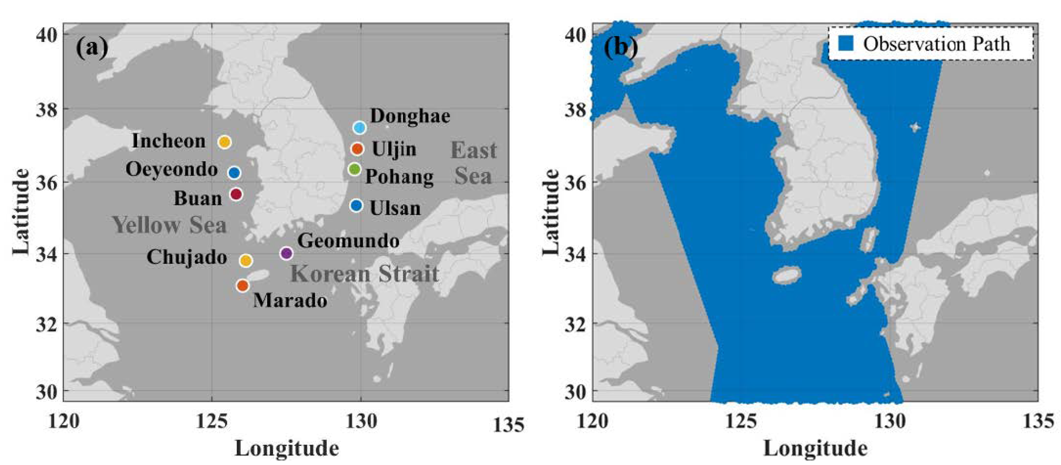
2. Study Area and Dataset
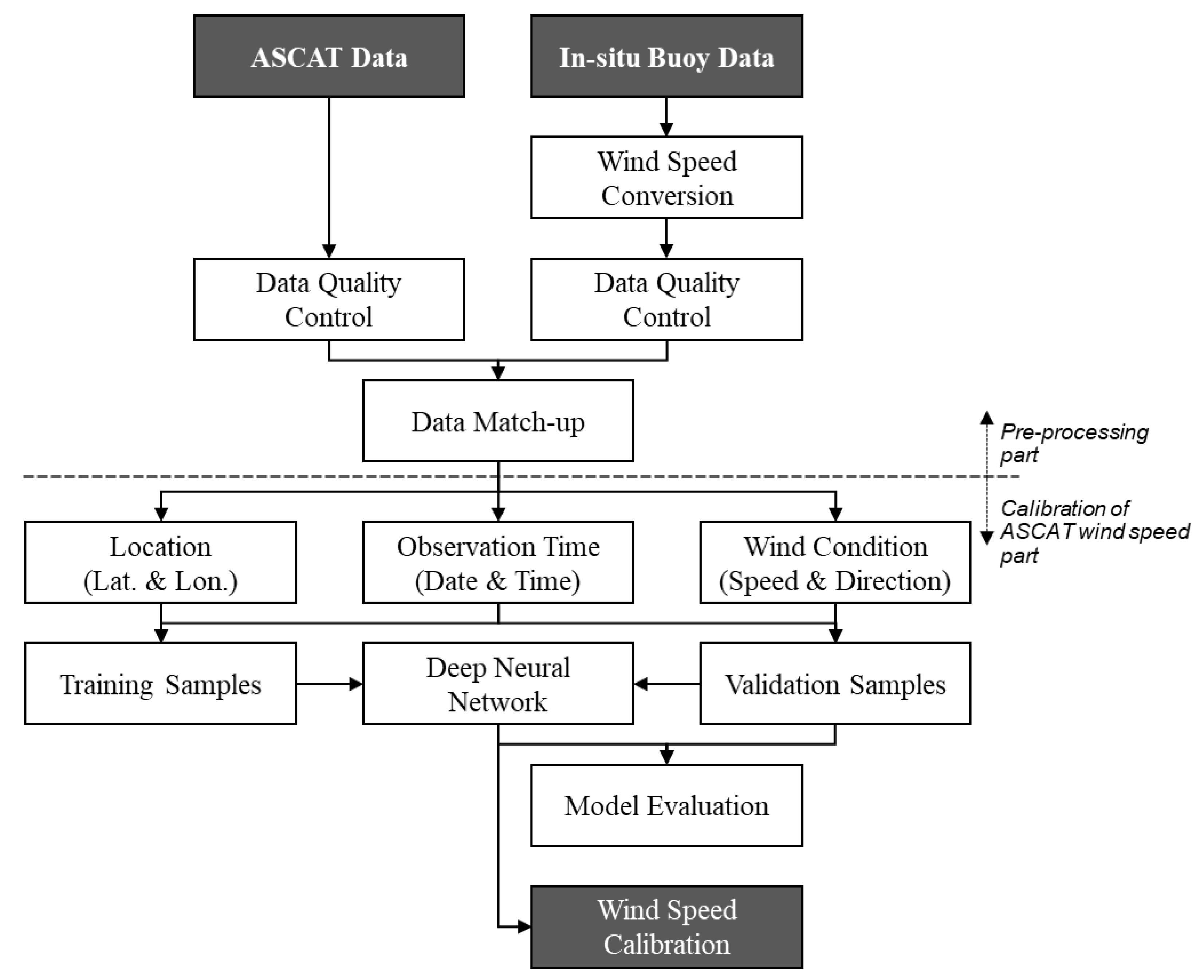
3. Methodology
3.1. Pre-Processing
3.2. Calibration of ASCAT wind Speed Using DNN
4. Results
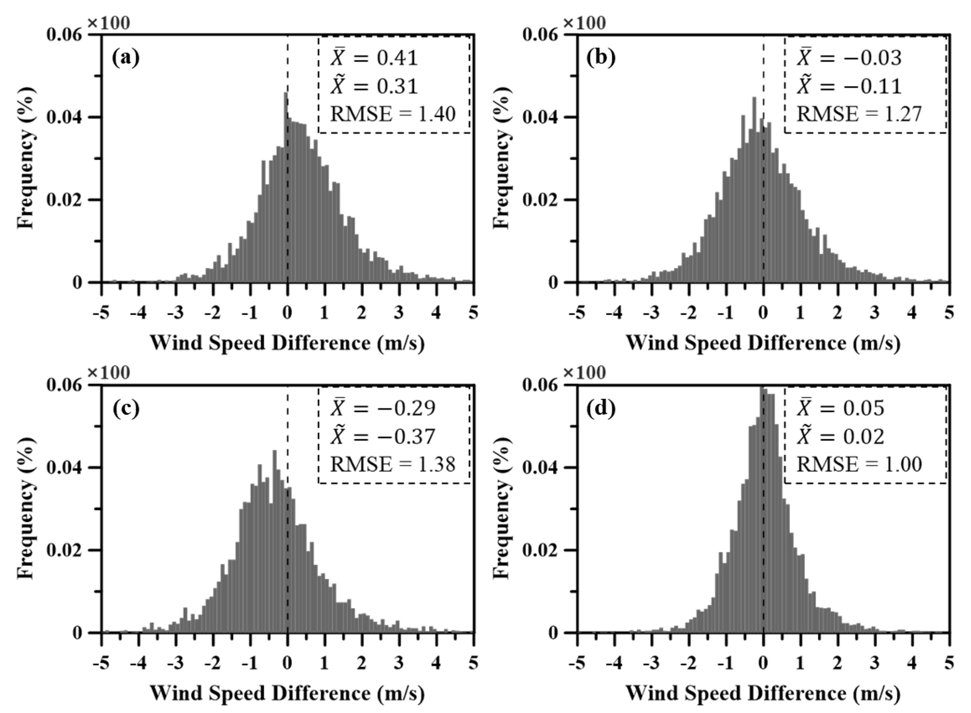
4.1. Pre-Processing Results
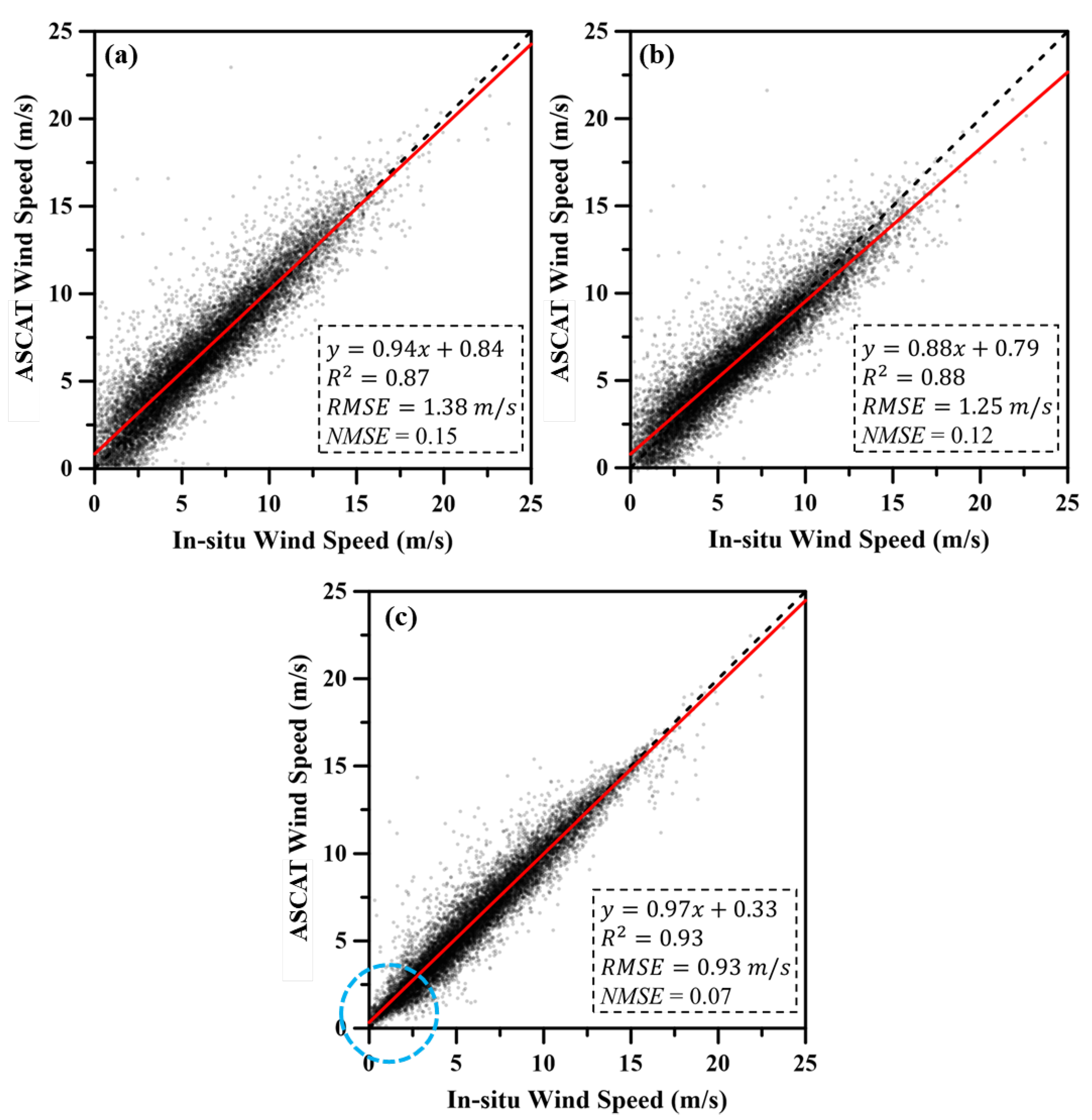
4.2. Comparison of Results by the DNN-Based Model and Other Calibration Methods
4.3. Consistency of DNN-Based Calibration Results
5. Discussion
6. Conclusions
Author Contributions
Funding
Institutional Review Board Statement
Informed Consent Statement
Data Availability Statement
Acknowledgments
Conflicts of Interest
References
- Jang, J.C.; Park, K.A.; Yang, D. Validation of Sea Surface Wind Estimated from KOMPSAT-5 Backscattering Coefficient Data. Korean J. Remote Sens. 2018, 34, 1383–1398. [Google Scholar]
- Son, D.; Jun, K.; Shim, J.S.; Kown, J.I.; Yoo, J. Validation of MetOp-B and Jason-2 Sea Surface Wind Data around the Korean Peninsula. Korea Soc. Coast. Disaster Prev. 2020, 7, 233–241. [Google Scholar] [CrossRef]
- Janssen, P.A.E.M. Quasi-Linear Theory of Wind-Wave Generation Applied to Wave Forecasting. J. Phys. Oceanogr. 1991, 21, 1631–1642. [Google Scholar] [CrossRef] [Green Version]
- Kara, A.B.; Metzger, E.J.; Bourassa, M.A. Ocean current and wave effects on wind stress drag coefficient over the global ocean. Geophys. Res. Lett. 2007, 34, 1–4. [Google Scholar] [CrossRef]
- Brostrom, G. On the influence of large wind farms on the upper ocean circulation. J. Mar. Syst. 2008, 74, 585–591. [Google Scholar] [CrossRef]
- Debernard, J.B.; Roed, L.P. Future wind, wave and storm surge climate in the Northern Seas: A revisit. Tellus A Dyn. Meteorol. Oceanogr. 2008, 60, 427–438. [Google Scholar] [CrossRef] [Green Version]
- Lee, C.M.; Orlic, M.; Poulain, P.M.; Cushman-Roisin, B. Introduction to special section: Recent advances in oceanography and marine meteorology of the Adriatic Sea. J. Geophys. Res. Ocean 2007, 112, 1–3. [Google Scholar] [CrossRef] [Green Version]
- Chelton, D.B.; Freilich, M.H.; Sienkiewicz, J.M.; Von Ahn, J.M. On the use of QuikSCAT scatterometer measurements of surface winds for marine weather prediction. Mon. Weather Rev. 2006, 134, 2055–2071. [Google Scholar] [CrossRef]
- Atlas, R.; Hoffman, R.N.; Leidner, S.M.; Sienkiewicz, J.; Yu, T.W.; Bloom, S.C.; Brin, E.; Ardizzone, J.; Terry, J.; Bungato, D.; et al. The effects of marine winds from scatterometer data on weather analysis and forecasting. Bull. Am. Meteorol. Soc. 2001, 82, 1965–1990. [Google Scholar] [CrossRef] [Green Version]
- Cavaleri, L.; Barbariol, F.; Benetazzo, A. Wind-Wave Modeling: Where We Are, Where to Go. J. Mar. Sci. Eng. 2020, 8, 260. [Google Scholar] [CrossRef] [Green Version]
- Ruiz-Salcines, P.; Salles, P.; Robles-Diaz, L.; Diaz-Hernandez, G.; Torres-Freyermuth, A.; Appendini, C.M. On the Use of Parametric Wind Models for Wind Wave Modeling under Tropical Cyclones. Water 2019, 11, 2044. [Google Scholar] [CrossRef] [Green Version]
- Choo, T.H.; Kim, Y.S.; Sim, S.B.; Son, J.K. Development of the Wind Wave Damage Predicting Functions in southern sea based on Annual Disaster Reports. J. Korea Acad. Ind. Coop. Soc. 2018, 19, 668–675. [Google Scholar]
- Zheng, C.W.; Li, C.Y.; Pan, J.; Liu, M.Y.; Xia, L.L. An overview of global ocean wind energy resource evaluations. Renew. Sustain. Energy Rev. 2016, 53, 1240–1251. [Google Scholar] [CrossRef]
- Li, J.; Wang, D.X.; Chen, J.; Yang, L. Comparison of remote sensing data with in-situ wind observation during the development of the South China Sea monsoon. Chin. J. Oceanol. Limnol. 2012, 30, 933–943. [Google Scholar] [CrossRef]
- Rashmi, R.; Aboobacker, V.M.; Vethamony, P.; John, M.P. Co-existence of wind seas and swells along the west coast of India during non-monsoon season. Ocean Sci. 2013, 9, 281–292. [Google Scholar] [CrossRef] [Green Version]
- Pickett, M.H.; Tang, W.Q.; Rosenfeld, L.K.; Wash, C.H. QuikSCAT satellite comparisons with nearshore buoy wind data off the US West Coast. J. Atmos. Ocean. Technol. 2003, 20, 1869–1879. [Google Scholar] [CrossRef] [Green Version]
- Hwang, P.A.; Teague, W.J.; Jacobs, G.A.; Wang, D.W. A statistical comparison of wind speed, wave height, and wave period derived from satellite altimeters and ocean buoys in the Gulf of Mexico region. J. Geophys. Res. Ocean 1998, 103, 10451–10468. [Google Scholar] [CrossRef] [Green Version]
- Kumar, S.V.V.A.; Nagababu, G.; Kumar, R. Comparative study of offshore winds and wind energy production derived from multiple scatterometers and met buoys. Energy 2019, 185, 599–611. [Google Scholar] [CrossRef]
- Ebuchi, N.; Graber, H.C.; Caruso, M.J. Evaluation of wind vectors observed by QuikSCAT/SeaWinds using ocean buoy data. J. Atmos. Ocean. Technol. 2002, 19, 2049–2062. [Google Scholar] [CrossRef]
- Satheesan, K.; Sarkar, A.; Parekh, A.; Kumar, M.R.R.; Kuroda, Y. Comparison of wind data from QuikSCAT and buoys in the Indian Ocean. Int. J. Remote Sens. 2007, 28, 2375–2382. [Google Scholar] [CrossRef]
- Carvalho, D.; Rocha, A.; Gomez-Gesteira, M.; Santos, C.S. Comparison of reanalyzed, analyzed, satellite-retrieved and NWP modelled winds with buoy data along the Iberian Peninsula coast. Remote Sens. Environ. 2014, 152, 480–492. [Google Scholar] [CrossRef]
- Gower, J.F.R. Intercalibration of wave and wind data from TOPEX POSEIDON and moored buoys off the west coast of Canada. J. Geophys. Res. Ocean 1996, 101, 3817–3829. [Google Scholar] [CrossRef]
- Jones, W.L.; Schroeder, L.C.; Boggs, D.H.; Bracalente, E.M.; Brown, R.A.; Dome, G.J.; Pierson, W.J.; Wentz, F.J. The SEASAT-A satellite scatterometer: The geophysical evaluation of remotely sensed wind vectors over the ocean. J. Geophys. Res. 1982, 87, 3297–3317. [Google Scholar] [CrossRef]
- Yang, J.G.; Zhang, J. Comparison of Oceansat-2 Scatterometer Wind Data with Global Moored Buoys and ASCAT Observation. Adv. Meteorol. 2019, 2019, 1651267. [Google Scholar] [CrossRef] [Green Version]
- Yang, X.F.; Li, X.F.; Pichel, W.G.; Li, Z.W. Comparison of Ocean Surface Winds From ENVISAT ASAR, MetOp ASCAT Scatterometer, Buoy Measurements, and NOGAPS Model. IEEE Trans. Geosci. Remote Sens. 2011, 49, 4743–4750. [Google Scholar] [CrossRef]
- Sharoni, S.M.H.; Reba, M.N.M.; Hossain, M.S. Tropical Cyclone Wind Speed Estimation From Satellite Altimeter-Derived Ocean Parameters. J. Geophys. Res. Ocean 2021, 126, e2020JC016988. [Google Scholar] [CrossRef]
- Wang, Z.X.; Stoffelen, A.; Zou, J.H.; Lin, W.M.; Verhoef, A.; Zhang, Y.; He, Y.J.; Lin, M.S. Validation of New Sea Surface Wind Products From Scatterometers Onboard the HY-2B and MetOp-C Satellites. IEEE Trans. Geosci. Remote Sens. 2020, 58, 4387–4394. [Google Scholar] [CrossRef]
- Witter, D.L.; Chelton, D.B. A Geosat Altimeter Wind-Speed Algorithm and a Method for Altimeter Wind-Speed Algorithm Development. J. Geophys. Res. Ocean 1991, 96, 8853–8860. [Google Scholar] [CrossRef]
- Horstmann, J.; Schiller, H.; Schulz-Stellenfleth, J.; Lehner, S. Global wind speed retrieval from SAR. IEEE Trans. Geosci. Remote Sens. 2003, 41, 2277–2286. [Google Scholar] [CrossRef] [Green Version]
- Ménard, Y.; Fu, L.-L.; Escudier, P.; Parisot, F.; Perbos, J.; Vincent, P.; Desai, S.; Haines, B.; Kunstmann, G. The Jason-1 Mission Special Issue: Jason-1 Calibration/Validation. Mar. Geod. 2003, 26, 131–146. [Google Scholar] [CrossRef]
- Abdalla, S.; Janssen, P.A.E.M.; Bidlot, J.R. Jason-2 OGDR Wind and Wave Products: Monitoring, Validation and Assimilation. Mar. Geod. 2010, 33, 239–255. [Google Scholar] [CrossRef]
- Yang, J.G.; Zhang, J.; Jia, Y.J.; Fan, C.Q.; Cui, W. Validation of Sentinel-3A/3B and Jason-3 Altimeter Wind Speeds and Significant Wave Heights Using Buoy and ASCAT Data. Remote Sens. 2020, 12, 2079. [Google Scholar] [CrossRef]
- Horstmann, J.; Koch, W.; Lehner, S. Ocean wind fields retrieved from the advanced synthetic aperture radar aboard ENVISAT. Ocean. Dyn. 2004, 54, 570–576. [Google Scholar] [CrossRef]
- Park, J.; Kim, D.W.; Jo, Y.H.; Kim, D. Accuracy Evaluation of Daily-gridded ASCAT Satellite Data Around the Korean Peninsula. Korean J. Remote Sens. 2018, 34, 213–225. [Google Scholar]
- Verhoef, A.; Portabella, M.; Stoffelen, A. High-Resolution ASCAT Scatterometer Winds Near the Coast. IEEE Trans. Geosci. Remote Sens. 2012, 50, 2481–2487. [Google Scholar] [CrossRef] [Green Version]
- Bentamy, A.; Croize-Fillon, D.; Perigaud, C. Characterization of ASCAT measurements based on buoy and QuikSCAT wind vector observations. Ocean Sci. 2008, 4, 265–274. [Google Scholar] [CrossRef] [Green Version]
- Ribal, A.; Young, I.R. Calibration and Cross Validation of Global Ocean Wind Speed Based on Scatterometer Observations. J. Atmos. Ocean. Technol. 2020, 37, 279–297. [Google Scholar] [CrossRef]
- Bentamy, A.; Fillon, D.C. Gridded surface wind fields from Metop/ASCAT measurements. Int. J. Remote Sens. 2012, 33, 1729–1754. [Google Scholar] [CrossRef] [Green Version]
- Jeong, J.Y.; Shim, J.S.; Lee, D.K.; Min, I.K.; Kwon, J.I. Validation of QuikSCAT Wind with Resolution of 12.5 km in the Vicinity of Korean Peninsula. Ocean Polar Res. 2008, 30, 47–58. [Google Scholar] [CrossRef] [Green Version]
- Kim, D.W.; Byun, H.R. Spatial and temporal distribution of wind resources over Korea. Atmosphere 2008, 18, 171–182. [Google Scholar]
- Kalra, R.; Deo, M.C. Derivation of coastal wind and wave parameters from offshore measurements of TOPEX satellite using ANN. Coast. Eng. 2007, 54, 187–196. [Google Scholar] [CrossRef]
- Huang, C.J.; Kuo, P.H. A Short-Term Wind Speed Forecasting Model by Using Artificial Neural Networks with Stochastic Optimization for Renewable Energy Systems. Energies 2018, 11, 2777. [Google Scholar] [CrossRef] [Green Version]
- Liu, Y.X.; Collett, I.; Morton, Y.J. Application of Neural Network to GNSS-R Wind Speed Retrieval. IEEE Trans. Geosci. Remote Sens. 2019, 57, 9756–9766. [Google Scholar] [CrossRef]
- Duan, J.K.; Zuo, H.C.; Bai, Y.L.; Duan, J.Z.; Chang, M.H.; Chen, B.L. Short-term wind speed forecasting using recurrent neural networks with error correction. Energy 2021, 217, 119397. [Google Scholar] [CrossRef]
- Kim, M.K.; Kim, Y.H.; Lee, W.S. Seasonal prediction of Korean regional climate from preceding large-scale climate indices. Int. J. Climatol. 2007, 27, 925–934. [Google Scholar] [CrossRef]
- Figa-Saldana, J.; Wilson, J.J.W.; Attema, E.; Gelsthorpe, R.; Drinkwater, M.R.; Stoffelen, A. The advanced scatterometer (ASCAT) on the meteorological operational (MetOp) platform: A follow on for European wind scatterometers. Can. J. Remote Sens. 2002, 28, 404–412. [Google Scholar] [CrossRef]
- Fairall, C.W.; Bradley, E.F.; Hare, J.E.; Grachev, A.A.; Edson, J.B. Bulk parameterization of air-sea fluxes: Updates and verification for the COARE algorithm. J. Clim. 2003, 16, 571–591. [Google Scholar] [CrossRef]
- Smith, S.D. Coefficients for Sea-Surface Wind Stress, Heat-Flux, and Wind Profiles as a Function of Wind-Speed and Temperature. J. Geophys. Res. Ocean 1988, 93, 15467–15472. [Google Scholar] [CrossRef]
- Byun, D.S.; Kim, H.; Lee, J.; Lee, E.; Park, K.A.; Woo, H.J. Converting Ieodo ocean research station wind speed observations to reference height data for real-time operational use. J. Koream Soc. Ocean. 2018, 23, 153–178. [Google Scholar]
- Mohandes, M.A.; Halawani, T.O.; Rehman, S.; Hussain, A.A. Support vector machines for wind speed prediction. Energy 2004, 29, 939–947. [Google Scholar] [CrossRef]
- Serdar, C.C.; Cihan, M.; Yücel, D.; Serdar, M.A. Sample size, power and effect size revisited: Simplified and practical approaches in pre-clinical, clinical and laboratory studies. Biochem. Med. 2021, 31, 010502. [Google Scholar] [CrossRef] [PubMed]
- Choo, T.H.; Kwak, K.S.; Ahn, S.H.; Yamg, D.U.; Son, J.K. Development for the function of Wind wave Damage Estimation at the Western Coastal Zone based on Disaster Statistics. J. Korea Acad. Ind. Coop. Soc. 2017, 18, 14–22. [Google Scholar]
- Choo, Y.M.; Chun, K.H.; Jeon, H.S.; Sim, S.B. A Predictive Model for Estimating Damage from Wind Waves during Coastal Storms. Water 2021, 13, 1322. [Google Scholar] [CrossRef]
- Kim, C.K.; Yum, S.S. Local meteorological and synoptic characteristics of fogs formed over Incheon international airport in the west coast of Korea. Adv. Atmos. Sci. 2010, 27, 761–776. [Google Scholar] [CrossRef]


| No. | Station Name | Abbr. Name | Lat. (Deg) | Lon. (Deg) | Observation Period | Height * (m) | Number of Observations |
|---|---|---|---|---|---|---|---|
| 1 | Oeyendo | OY | 36.25 | 125.75 | Oct 2012–Dec 2019 | 3.60 | 66,234 |
| 2 | Marado | MA | 33.08 | 126.03 | Oct 2012–Dec 2019 | 4.60 | 65,371 |
| 3 | Chujado | CJ | 33.79 | 126.14 | Jan 2014–Dec 2019 | 4.10 | 46,514 |
| 4 | Geomundo | GM | 34.00 | 127.50 | Jan 2012–Dec 2019 | 4.70 | 65,812 |
| 5 | Pohang | PH | 36.35 | 129.78 | Oct 2012–Dec 2019 | 4.60 | 65,389 |
| 6 | Donghae | DH | 37.48 | 129.95 | Oct 2012–Dec 2019 | 4.10 | 64,964 |
| 7 | Buan | BU | 35.66 | 125.81 | Dec 2015–Jul 2019 | 4.70 | 30,059 |
| 8 | Ulsan | US | 35.35 | 129.84 | Dec 2015–Jul 2019 | 4.10 | 29,668 |
| 9 | Uljin | UJ | 36.91 | 129.87 | Dec 2015–Jul 2019 | 4.10 | 30,975 |
| 10 | Incheon | IC | 37.09 | 125.43 | Dec 2015–Jul 2019 | 4.00 | 28,972 |
| total | 493,958 |
| No. | OY | MA | CJ | GM | PH | DH | BU | US | UJ | IC | Total |
|---|---|---|---|---|---|---|---|---|---|---|---|
| Number of Matched Data | 1924 | 1677 | 1369 | 1989 | 1821 | 1795 | 930 | 852 | 875 | 907 | 14,139 |
| Matching Ratio | 2.90 | 2.57 | 2.94 | 3.02 | 2.78 | 2.76 | 3.09 | 2.87 | 2.82 | 3.13 | 2.86 |
| Method | Input Variable for Finding the Best Fit Function | Results | |||
|---|---|---|---|---|---|
| Mean | Median | RMSE | Kurtosis | ||
| Before calibrated | - | 0.41 | 0.31 | 1.40 | 7.04 |
| Linear Regression-1 | Wind speed | 0.02 | −0.08 | 1.34 | 6.85 |
| Linear Regression-2 | Wind speed + Wind direction + Location + Date + Time | −0.03 | −0.11 | 1.27 | 2.97 |
| SVR | Wind speed + Wind direction + Location + Date + Time | −0.29 | −0.37 | 1.38 | 6.24 |
| DNN-1 | Wind speed + Wind direction | −0.04 | −0.13 | 1.26 | 9.37 |
| DNN-2 | Wind speed + Location | −0.13 | −0.21 | 1.22 | 4.39 |
| DNN-3 | Wind speed + Date + Time | 0.12 | 0.04 | 1.25 | 9.24 |
| DNN-4 | Wind speed + Wind direction + Location + Date + Time | 0.05 | 0.02 | 1.00 | 12.54 |
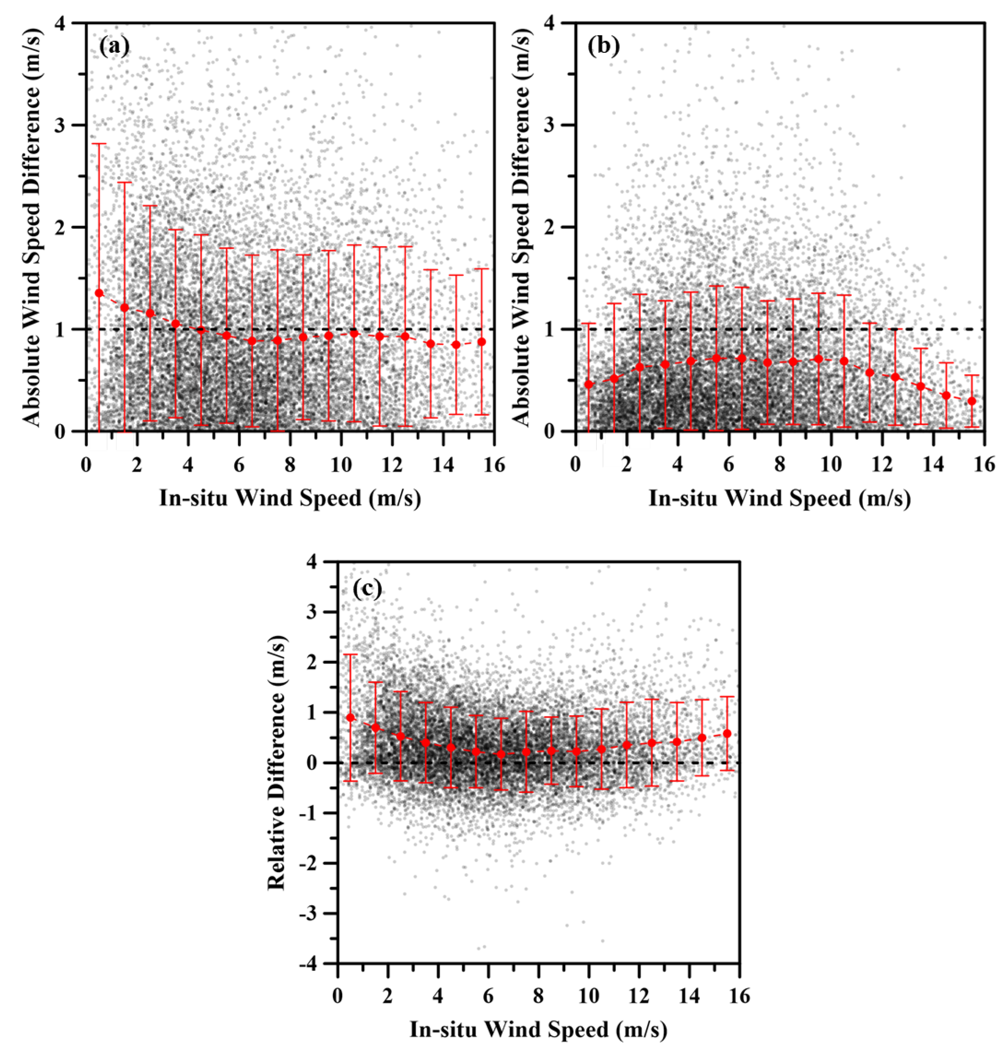
| Wind Speed (m/s) | Before Calibration | After Calibration | ||
|---|---|---|---|---|
| Mean of △WS (m/s) | Std. of △WS (m/s) | Mean of △WS (m/s) | Std. of △WS (m/s) | |
| 0–1 | 1.35 | 1.46 | 0.46 | 0.60 |
| 1–2 | 1.21 | 1.23 | 0.52 | 0.74 |
| 2–3 | 1.16 | 1.05 | 0.63 | 0.71 |
| 3–4 | 1.05 | 0.92 | 0.65 | 0.62 |
| 4–5 | 0.99 | 0.93 | 0.69 | 0.68 |
| 5–6 | 0.94 | 0.86 | 0.72 | 0.71 |
| 6–7 | 0.89 | 0.84 | 0.71 | 0.70 |
| 7–8 | 0.89 | 0.89 | 0.67 | 0.60 |
| 8–9 | 0.92 | 0.81 | 0.68 | 0.61 |
| 9–10 | 0.94 | 0.83 | 0.71 | 0.64 |
| 10–11 | 0.96 | 0.87 | 0.69 | 0.65 |
| 11–12 | 0.93 | 0.88 | 0.57 | 0.48 |
| 12–13 | 0.93 | 0.88 | 0.53 | 0.47 |
| 13–14 | 0.86 | 0.73 | 0.44 | 0.37 |
| 14–15 | 0.85 | 0.68 | 0.35 | 0.32 |
| 15–16 | 0.88 | 0.71 | 0.30 | 0.25 |
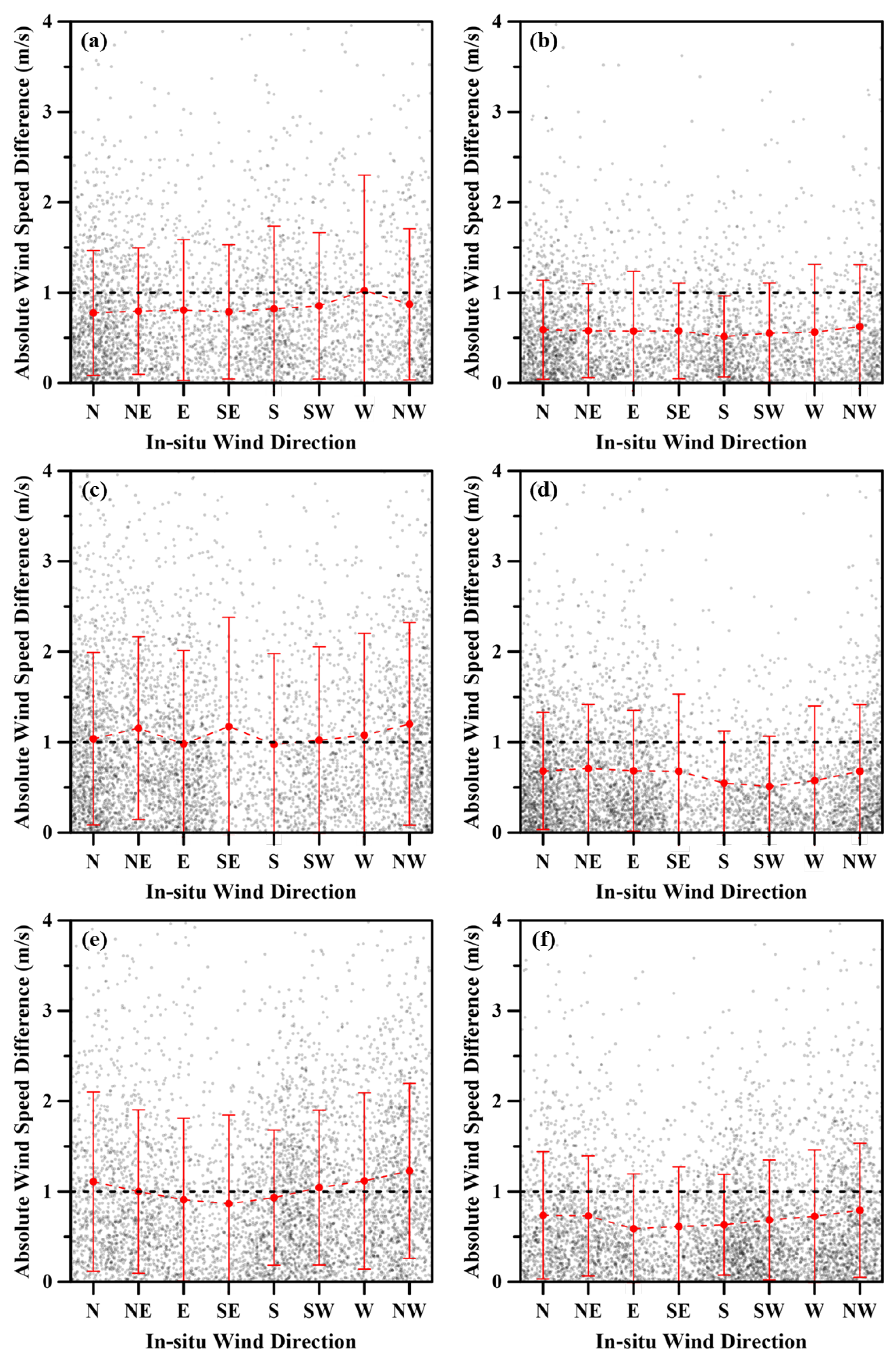
| Before Calibration | After Calibration | |||||||||||
|---|---|---|---|---|---|---|---|---|---|---|---|---|
| Yellow Sea | Korean Strait | East Sea | Yellow Sea | Korean Strait | East Sea | |||||||
| Wind Direction | Mean △WS (m/s) | Std. △WS (m/s) | Mean △WS (m/s) | Std. △WS (m/s) | Mean △WS (m/s) | Std. △WS (m/s) | Mean △WS (m/s) | Std. △WS (m/s) | Mean △WS (m/s) | Std. △WS (m/s) | Mean △WS (m/s) | Std. △WS (m/s) |
| North | 0.78 | 0.69 | 1.04 | 0.95 | 1.11 | 0.99 | 0.59 | 0.55 | 0.68 | 0.65 | 0.74 | 0.70 |
| North-east | 0.80 | 0.70 | 1.16 | 1.01 | 1.00 | 0.90 | 0.58 | 0.52 | 0.71 | 0.71 | 0.73 | 0.66 |
| East | 0.81 | 0.78 | 0.98 | 1.03 | 0.91 | 0.90 | 0.58 | 0.66 | 0.68 | 0.67 | 0.59 | 0.61 |
| South-east | 0.79 | 0.74 | 1.17 | 1.21 | 0.87 | 0.98 | 0.58 | 0.53 | 0.68 | 0.86 | 0.61 | 0.66 |
| South | 0.82 | 0.92 | 0.98 | 1.00 | 0.93 | 0.75 | 0.51 | 0.45 | 0.55 | 0.58 | 0.63 | 0.56 |
| South-west | 0.85 | 0.81 | 1.02 | 1.03 | 1.04 | 0.86 | 0.55 | 0.56 | 0.51 | 0.55 | 0.68 | 0.66 |
| West | 1.02 | 1.28 | 1.08 | 1.13 | 1.12 | 0.98 | 0.56 | 0.75 | 0.58 | 0.83 | 0.73 | 0.73 |
| North-west | 0.87 | 0.84 | 1.20 | 1.12 | 1.23 | 0.97 | 0.62 | 0.69 | 0.68 | 0.74 | 0.79 | 0.74 |
Publisher’s Note: MDPI stays neutral with regard to jurisdictional claims in published maps and institutional affiliations. |
© 2021 by the authors. Licensee MDPI, Basel, Switzerland. This article is an open access article distributed under the terms and conditions of the Creative Commons Attribution (CC BY) license (https://creativecommons.org/licenses/by/4.0/).
Share and Cite
Park, S.-H.; Yoo, J.; Son, D.; Kim, J.; Jung, H.-S. Improved Calibration of Wind Estimates from Advanced Scatterometer MetOp-B in Korean Seas Using Deep Neural Network. Remote Sens. 2021, 13, 4164. https://doi.org/10.3390/rs13204164
Park S-H, Yoo J, Son D, Kim J, Jung H-S. Improved Calibration of Wind Estimates from Advanced Scatterometer MetOp-B in Korean Seas Using Deep Neural Network. Remote Sensing. 2021; 13(20):4164. https://doi.org/10.3390/rs13204164
Chicago/Turabian StylePark, Sung-Hwan, Jeseon Yoo, Donghwi Son, Jinah Kim, and Hyung-Sup Jung. 2021. "Improved Calibration of Wind Estimates from Advanced Scatterometer MetOp-B in Korean Seas Using Deep Neural Network" Remote Sensing 13, no. 20: 4164. https://doi.org/10.3390/rs13204164