
Spatio-Temporal Simulation of Mangrove Forests under Different Scenarios: A Case Study of Mangrove Protected Areas, Hainan Island, China


Abstract
:1. Introduction
2. Materials
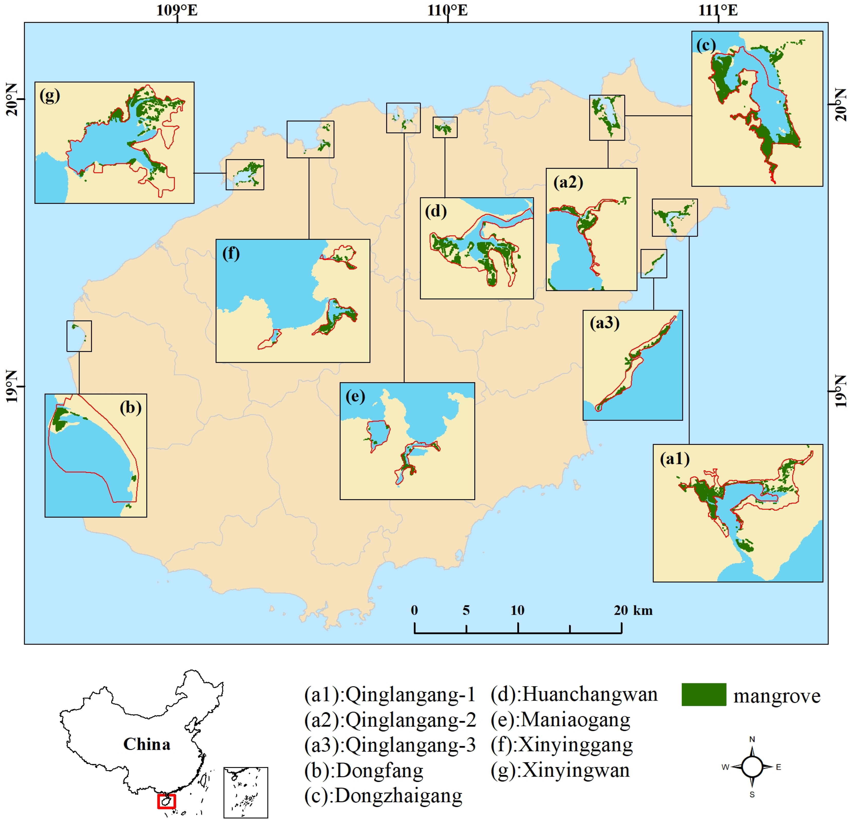
2.1. Study Area
2.2. Data Sources
3. Methods
3.1. CLUE-S Model
3.2. Model Validation Indices
3.3. Scenario Setting
4. Results
4.1. Simulation Accuracy of Spatial Characteristic
4.2. Simulation Results and Accuracy Assessment
4.3. Applicability of Driving Factors
4.4. Spatio-Temporal Distribution and Change Trends of Mangrove Forests under Different Scenarios
4.4.1. Spatio-Temporal Distribution of Mangrove Forests
4.4.2. Temporal Change Trends of Mangrove Forests
4.4.3. Spatial Change Trends of Mangrove Forests
5. Discussion
5.1. Comparison of the Spatio-Temporal Simulation Methods of Mangrove Forests
5.2. Future Changes of Mangrove Forests in Hainan Island
5.3. Limitations and Future Perspective of the Study
6. Conclusions
Supplementary Materials
Author Contributions
Funding
Data Availability Statement
Acknowledgments
Conflicts of Interest
References
- Giri, C. Recent Advancement in Mangrove Forests Mapping and Monitoring of the World Using Earth Observation Satellite Data. Remote Sens. 2021, 13, 563. [Google Scholar] [CrossRef]
- Mumby, P.J.; Edwards, A.J.; Arias-Gonzalez, J.E.; Lindeman, K.C.; Blackwell, P.G.; Gall, A.; Gorczynska, M.I.; Harborne, A.R.; Pescod, C.L.; Renken, H.; et al. Mangroves enhance the biomass of coral reef fish communities in the Caribbean. Nature 2004, 427, 533–536. [Google Scholar] [CrossRef] [PubMed] [Green Version]
- Barbier, E.B. Natural barriers to natural disasters: Replanting mangroves after the tsunami. Front. Ecol. Environ. 2006, 4, 124–131. [Google Scholar] [CrossRef]
- Walters, B.B.; Ronnback, P.; Kovacs, J.M.; Crona, B.; Hussain, S.A.; Badola, R.; Primavera, J.H.; Barbier, E.; Dahdouh-Guebas, F. Ethnobiology, socio-economics and management of mangrove forests: A review. Aquat. Bot. 2008, 89, 220–236. [Google Scholar] [CrossRef] [Green Version]
- Barbier, E.B.; Hacker, S.D.; Kennedy, C.; Koch, E.W.; Stier, A.C.; Silliman, B.R. The value of estuarine and coastal ecosystem services. Ecol. Monogr. 2011, 81, 169–193. [Google Scholar] [CrossRef]
- Donato, D.C.; Kauffman, J.B.; Murdiyarso, D.; Kurnianto, S.; Stidham, M.; Kanninen, M. Mangroves among the most carbon-rich forests in the tropics. Nat. Geosci. 2011, 4, 293–297. [Google Scholar] [CrossRef]
- Vo, Q.T.; Kuenzer, C.; Vo, Q.M.; Moder, F.; Oppelt, N. Review of valuation methods for mangrove ecosystem services. Ecol. Indic. 2012, 23, 431–446. [Google Scholar] [CrossRef]
- Goldberg, L.; Lagomasino, D.; Thomas, N.; Fatoyinbo, T. Global declines in human-driven mangrove loss. Glob. Chang. Biol. 2020, 26, 5844–5855. [Google Scholar] [CrossRef]
- Yirga, A.; Addisu Legesse, S.; Mekuriaw, A. Carbon Stock and Mitigation Potentials of Zeghie Natural Forest for Climate Change Disaster Reduction, Blue Nile Basin, Ethiopia. Earth Syst. Environ. 2020, 4, 27–41. [Google Scholar] [CrossRef]
- Valipour, M.; Bateni, S.M.; Jun, C. Global Surface Temperature: A New Insight. Climate 2021, 9, 81. [Google Scholar] [CrossRef]
- Richards, D.R.; Friess, D.A. Rates and drivers of mangrove deforestation in Southeast Asia, 2000-2012. Proc. Natl. Acad. Sci. USA 2016, 113, 344–349. [Google Scholar] [CrossRef] [Green Version]
- Friess, D.A.; Thompson, B.S.; Brown, B.; Amir, A.A.; Cameron, C.; Koldewey, H.J.; Sasmito, S.D.; Sidik, F. Policy challenges and approaches for the conservation of mangrove forests in Southeast Asia. Conserv. Biol. 2016, 30, 933–949. [Google Scholar] [CrossRef]
- Thomas, N.; Lucas, R.; Bunting, P.; Hardy, A.; Rosenqvist, A.; Simard, M. Distribution and drivers of global mangrove forest change, 1996–2010. PLoS ONE 2017, 12, e0179302. [Google Scholar] [CrossRef] [Green Version]
- Murakami, H.; Delworth, T.L.; Cooke, W.F.; Zhao, M.; Xiang, B.Q.; Hsu, P.C. Detected climatic change in global distribution of tropical cyclones. Proc. Natl. Acad. Sci. USA 2020, 117, 10706–10714. [Google Scholar] [CrossRef] [PubMed]
- Alongi, D.M. Present state and future of the world’s mangrove forests. Environ. Conserv. 2002, 29, 331–349. [Google Scholar] [CrossRef] [Green Version]
- Mayaux, P.; Holmgren, P.; Achard, F.; Eva, H.; Stibig, H.; Branthomme, A. Tropical forest cover change in the 1990s and options for future monitoring. Philos. Trans. R. Soc. B-Biol. Sci. 2005, 360, 373–384. [Google Scholar] [CrossRef] [Green Version]
- Hamilton, S.E.; Casey, D. Creation of a high spatio-temporal resolution global database of continuous mangrove forest cover for the 21st century (CGMFC-21). Glob. Ecol. Biogeogr. 2016, 25, 729–738. [Google Scholar] [CrossRef]
- Conchedda, G.; Durieux, L.; Mayaux, P. An object-based method for mapping and change analysis in mangrove ecosystems. ISPRS J. Photogramm. Remote Sens. 2008, 63, 578–589. [Google Scholar] [CrossRef]
- Giri, C.; Ochieng, E.; Tieszen, L.L.; Zhu, Z.; Singh, A.; Loveland, T.; Masek, J.; Duke, N. Status and distribution of mangrove forests of the world using earth observation satellite data. Glob. Ecol. Biogeogr. 2011, 20, 154–159. [Google Scholar] [CrossRef]
- Nascimento, W.R.; Souza, P.W.M.; Proisy, C.; Lucas, R.M.; Rosenqvist, A. Mapping changes in the largest continuous Amazonian mangrove belt using object-based classification of multisensor satellite imagery. Estuar. Coast. Shelf Sci. 2013, 117, 83–93. [Google Scholar] [CrossRef]
- Jia, M.M. Remote Sensing Analysis of China’ Mangrove Forests Dynamic During 1973 to 2013; University of Chinese Academy of Sciences: Beijing, China, 2014. [Google Scholar]
- Chen, B.Q.; Xiao, X.M.; Li, X.P.; Pan, L.H.; Doughty, R.; Ma, J.; Dong, J.W.; Qin, Y.W.; Zhao, B.; Wu, Z.X.; et al. A mangrove forest map of China in 2015: Analysis of time series Landsat 7/8 and Sentinel-1A imagery in Google Earth Engine cloud computing platform. ISPRS J. Photogramm. Remote Sens. 2017, 131, 104–120. [Google Scholar] [CrossRef]
- Bunting, P.; Rosenqvist, A.; Lucas, R.M.; Rebelo, L.M.; Hilarides, L.; Thomas, N.; Hardy, A.; Itoh, T.; Shimada, M.; Finlayson, C.M. The Global Mangrove WatchA New 2010 Global Baseline of Mangrove Extent. Remote Sens. 2018, 10, 1669. [Google Scholar] [CrossRef] [Green Version]
- Suyadi; Gao, J.; Lundquist, C.J.; Schwendenmann, L. Characterizing landscape patterns in changing mangrove ecosystems at high, latitudes using spatial metrics. Estuar. Coast. Shelf Sci. 2018, 215, 1–10. [Google Scholar] [CrossRef]
- Jia, M.M.; Wang, Z.M.; Zhang, Y.Z.; Mao, D.H.; Wang, C. Monitoring loss and recovery of mangrove forests during 42 years: The achievements of mangrove conservation in China. Int. J. Appl. Earth Obs. Geoinf. 2018, 73, 535–545. [Google Scholar]
- Buitre, M.J.C.; Zhang, H.S.; Lin, H. The Mangrove Forests Change and Impacts from Tropical Cyclones in the Philippines Using Time Series Satellite Imagery. Remote Sens. 2019, 11, 688. [Google Scholar] [CrossRef] [Green Version]
- Liao, J.J.; Zhen, J.N.; Zhang, L.; Metternicht, G. Understanding Dynamics of Mangrove Forest on Protected Areas of Hainan Island, China: 30 Years of Evidence from Remote Sensing. Sustainability 2019, 11, 5356. [Google Scholar] [CrossRef] [Green Version]
- Chamberlain, D.; Phinn, S.; Possingham, H. Remote Sensing of Mangroves and Estuarine Communities in Central Queensland, Australia. Remote Sens. 2020, 12, 197. [Google Scholar] [CrossRef] [Green Version]
- Guo, Y.J.; Liao, J.J.; Shen, G.Z. Mapping Large-Scale Mangroves along the Maritime Silk Road from 1990 to 2015 Using a Novel Deep Learning Model and Landsat Data. Remote Sens. 2021, 13, 245. [Google Scholar] [CrossRef]
- Anwar, M.S.; Takewaka, S. Analyses on phenological and morphological variations of mangrove forests along the southwest coast of Bangladesh. J. Coast. Conserv. 2014, 18, 339–357. [Google Scholar] [CrossRef]
- Berlanga-Robles, C.A.; Ruiz-Luna, A.; Villanueva, M.R.N. Seasonal trend analysis (STA) of MODIS vegetation index time series for the mangrove canopy of the Teacapan-Agua Brava lagoon system, Mexico. Giscience Remote Sens. 2019, 56, 338–361. [Google Scholar]
- Le, H.T.; Tran, T.V.; Gyeltshen, S.; Nguyen, C.P.T.; Tran, D.X.; Luu, T.H.; Duong, M.B. Characterizing Spatiotemporal Patterns of Mangrove Forests in Can Gio Biosphere Reserve Using Sentinel-2 Imagery. Appl. Sci. Basel 2020, 10, 4058. [Google Scholar] [CrossRef]
- Zhu, B.; Liao, J.; Shen, G. Combining time series and land cover data for analyzing spatio-temporal changes in mangrove forests: A case study of Qinglangang Nature Reserve, Hainan, China. Ecol. Indic. 2021, 131, 108135. [Google Scholar] [CrossRef]
- Jiang, W.G.; Yuan, L.H.; Wang, W.J.; Cao, R.; Zhang, Y.F.; Shen, W.M. Spatio-temporal analysis of vegetation variation in the Yellow River Basin. Ecol. Indic. 2015, 51, 117–126. [Google Scholar] [CrossRef]
- Stephenne, N.; Lambin, E.F. A dynamic simulation model of land-use changes in Sudano-sahelian countries of Africa (SALU). Agric. Ecosyst Env. 2001, 85, 145–161. [Google Scholar] [CrossRef]
- Delgado-Matas, C.; Pukkala, T. Optimisation of the traditional land-use system in the Angolan highlands using linear programming. Int J. Sustain. Dev. World Ecol. 2014, 21, 138–148. [Google Scholar] [CrossRef]
- Taromi, R.; DuRoss, M.; Chen, B.T.; Faghri, A.; Li, M.X.; DeLiberty, T. A multiobjective land development optimization model: The case of New Castle County, Delaware. Transp. Plan. Technol. 2015, 38, 277–304. [Google Scholar] [CrossRef]
- Saysel, A.K.; Barlas, Y.; Yenigun, O. Environmental sustainability in an agricultural development project: A system dynamics approach. J. Environ. Manag. 2002, 64, 247–260. [Google Scholar] [CrossRef] [Green Version]
- Liu, X.P.; Ou, J.P.; Li, X.; Ai, B. Combining system dynamics and hybrid particle swarm optimization for land use allocation. Ecol. Model. 2013, 257, 11–24. [Google Scholar] [CrossRef]
- Chen, C.F.; Son, N.T.; Chang, N.B.; Chen, C.R.; Chang, L.Y.; Valdez, M.; Centeno, G.; Thompson, C.A.; Aceituno, J.L. Multi-Decadal Mangrove Forest Change Detection and Prediction in Honduras, Central America, with Landsat Imagery and a Markov Chain Model. Remote Sens. 2013, 5, 6408–6426. [Google Scholar] [CrossRef] [Green Version]
- Wu, D.Q.; Liu, J.; Zhang, G.S.; Ding, W.J.; Wang, W.; Wang, R.Q. Incorporating spatial autocorrelation into cellular automata model: An application to the dynamics of Chinese tamarisk (Tamarix chinensis Lour.). Ecol. Model. 2009, 220, 3490–3498. [Google Scholar] [CrossRef]
- Basse, R.M.; Omrani, H.; Charif, O.; Gerber, P.; Bodis, K. Land use changes modelling using advanced methods: Cellular automata and artificial neural networks. The spatial and explicit representation of land cover dynamics at the cross-border region scale. Appl. Geogr. 2014, 53, 160–171. [Google Scholar] [CrossRef]
- Castella, J.C.; Verburg, P.H. Combination of process-oriented and pattern-oriented models of land-use change in a mountain area of Vietnam. Ecol. Model. 2007, 202, 410–420. [Google Scholar] [CrossRef]
- Liu, X.P.; Liang, X.; Li, X.; Xu, X.C.; Ou, J.P.; Chen, Y.M.; Li, S.Y.; Wang, S.J.; Pei, F.S. A future land use simulation model (FLUS) for simulating multiple land use scenarios by coupling human and natural effects. Landsc. Urban. Plan. 2017, 168, 94–116. [Google Scholar] [CrossRef]
- Roetter, R.P.; Hoanh, C.T.; Laborte, A.G.; Van Keulen, H.; Van Ittersum, M.K.; Dreiser, C.; Van Diepen, C.A.; De Ridder, N.; Van Laar, H.H. Integration of Systems Network (SysNet) tools for regional land use scenario analysis in Asia. Environ. Model. Softw. 2005, 20, 291–307. [Google Scholar] [CrossRef]
- Verburg, P.H.; Soepboer, W.; Veldkamp, A.; Limpiada, R.; Espaldon, V.; Mastura, S.S.A. Modeling the spatial dynamics of regional land use: The CLUE-S model. Environ. Manag. 2002, 30, 391–405. [Google Scholar] [CrossRef]
- Mukhopadhyay, A.; Mondal, P.; Barik, J.; Chowdhury, S.M.; Ghosh, T.; Hazra, S. Changes in mangrove species assemblages and future prediction of the Bangladesh Sundarbans using Markov chain model and cellular automata. Environ. Sci. Process. Impacts 2015, 17, 1111–1117. [Google Scholar] [CrossRef]
- Bozkaya, A.G.; Balcik, F.B.; Goksel, C.; Esbah, H. Forecasting land-cover growth using remotely sensed data: A case study of the Igneada protection area in Turkey. Environ. Monit. Assess. 2015, 187, 59. [Google Scholar] [CrossRef]
- DasGupta, R.; Hashimoto, S.; Okuro, T.; Basu, M. Scenario-based land change modelling in the Indian Sundarban delta: An exploratory analysis of plausible alternative regional futures. Sustain. Sci. 2019, 14, 221–240. [Google Scholar] [CrossRef]
- Tajbakhsh, A.; Karimi, A.; Zhang, A.L. Modeling land cover change dynamic using a hybrid model approach in Qeshm Island, Southern Iran. Environ. Monit. Assess. 2020, 192, 303. [Google Scholar] [CrossRef]
- Lin, Y.-P.; Chu, H.-J.; Wu, C.-F.; Verburg, P.H. Predictive ability of logistic regression, auto-logistic regression and neural network models in empirical land-use change modeling—A case study. Int. J. Geogr. Inf. Sci. 2011, 25, 65–87. [Google Scholar] [CrossRef] [Green Version]
- Jiang, W.G.; Chen, Z.; Lei, X.; He, B.; Jia, K.; Zhang, Y.F. Simulation of urban agglomeration ecosystem spatial distributions under different scenarios: A case study of the Changsha-Zhuzhou-Xiangtan urban agglomeration. Ecol. Eng. 2016, 88, 112–121. [Google Scholar] [CrossRef]
- Peng, K.F.; Jiang, W.G.; Deng, Y.; Liu, Y.H.; Wu, Z.F.; Chen, Z. Simulating wetland changes under different scenarios based on integrating the random forest and CLUE-S models: A case study of Wuhan Urban Agglomeration. Ecol. Indic. 2020, 117, 106671. [Google Scholar] [CrossRef]
- Mas, J.F.; Kolb, M.; Paegelow, M.; Olmedo, M.T.C.; Houet, T. Inductive pattern-based land use/cover change models: A comparison of four software packages. Environ. Model. Softw. 2014, 51, 94–111. [Google Scholar] [CrossRef] [Green Version]
- Tang, F.; Fu, M.C.; Wang, L.; Zhang, P.T. Land-use change in Changli County, China: Predicting its spatio-temporal evolution in habitat quality. Ecol. Indic. 2020, 117, 106719. [Google Scholar] [CrossRef]
- Mei, Z.X.; Wu, H.; Li, S.Y. Simulating land-use changes by incorporating spatial autocorrelation and self-organization in CLUE-S modeling: A case study in Zengcheng District, Guangzhou, China. Front. Earth Sci. 2018, 12, 299–310. [Google Scholar] [CrossRef]
- Jiang, W.G.; Chen, Z.; Lei, X.; Jia, K.; Wu, Y.F. Simulating urban land use change by incorporating an autologistic regression model into a CLUE-S model. J. Geogr. Sci. 2015, 25, 836–850. [Google Scholar] [CrossRef] [Green Version]
- Li, Z.; Jiang, W.G.; Wang, W.J.; Lei, X.; Deng, Y. Exploring spatial-temporal change and gravity center movement of construction land in the Chang-Zhu-Tan urban agglomeration. J. Geogr. Sci. 2019, 29, 1363–1380. [Google Scholar] [CrossRef] [Green Version]
- Peng, K.F.; Jiang, W.G.; Ling, Z.Y.; Hou, P.; Deng, Y.W. Evaluating the potential impacts of land use changes on ecosystem service value under multiple scenarios in support of SDG reporting: A case study of the Wuhan urban agglomeration. J. Clean. Prod. 2021, 307, 127321. [Google Scholar] [CrossRef]
- Piao, S.L.; Fang, J.Y. Dynamic vegetation cover change over the last 18 years in China. Quat. Sci. 2001, 21, 294–302. [Google Scholar]
- Besag, J.E. Nearest-Neighbour Systems and the Auto-Logistic Model for Binary Data. J. R. Stat. Soc. Ser. B Stat. Methodol. 1972, 34, 75–83. [Google Scholar] [CrossRef]
- Wang, W.Q.; Wang, M. The Mangroves of China; Science Press: Beijing, China, 2007. [Google Scholar]
- Xin, X.; Song, X.Q.; Lei, J.R.; Fang, Z.S.; Meng, Q.W. Mangrove Plants Resources and Its Conservation Strategies on Hainan. J. Trop. Biol. 2016, 7, 477–483. [Google Scholar]
- Chen, H.X.; Chen, E.Y. Distribution of Mangrove in Hainan Island at Present. J. Trop Oceanogr. 1985, 1985, 74–79. [Google Scholar]
- Zhen, J.N. Monitoring and Dynamic Analysis of Mangrove Forests in Hainan Island using Multi-Temporal Remote Sensing Images; University of Chinese Academy of Sciences: Beijing, China, 2019. [Google Scholar]
- Liu, H.Q.; Huete, A. A feedback based modification of the NDVI to minimize canopy background and atmospheric noise. ITGRS 1995, 33, 457–465. [Google Scholar] [CrossRef]
- Cao, R.; Jiang, W.G.; Yuan, L.H.; Wang, W.J.; Lv, Z.L.; Chen, Z. Inter-annual variations in vegetation and their response to climatic factors in the upper catchments of the Yellow River from 2000 to 2010. J. Geogr. Sci. 2014, 24, 963–979. [Google Scholar] [CrossRef] [Green Version]
- Lv, J.X.; Jiang, W.G.; Wang, W.J.; Wu, Z.F.; Liu, Y.H.; Wang, X.Y.; Li, Z. Wetland Loss Identification and Evaluation Based on Landscape and Remote Sensing Indices in Xiong’an New Area. Remote Sens. 2019, 11, 2834. [Google Scholar] [CrossRef] [Green Version]
- Chen, Y.; Li, X.; Su, W.; Li, Y. Simulating the optimal land-use pattern in the farming-pastoral transitional zone of Northern China. Comput. Environ. Urban. Syst. 2008, 32, 407–414. [Google Scholar] [CrossRef]
- Zhang, L.P.; Zhang, S.W.; Huang, Y.J.; Cao, M.; Huang, Y.F.; Zhang, H.Y. Exploring an Ecologically Sustainable Scheme for Landscape Restoration of Abandoned Mine Land: Scenario-Based Simulation Integrated Linear Programming and CLUE-S Model. Int. J. Environ. Res. Public Health 2016, 13, 354. [Google Scholar] [CrossRef] [Green Version]
- Zhao, X.; Li, S.; Pu, J.; Miao, P.; Wang, Q.; Tan, K. Optimization of the National Land Space Based on the Coordination of Urban-Agricultural-Ecological Functions in the Karst Areas of Southwest China. Sustainability 2019, 11, 6752. [Google Scholar] [CrossRef] [Green Version]
- Zhang, Z.; Hu, B.; Jiang, W.; Qiu, H. Identification and scenario prediction of degree of wetland damage in Guangxi based on the CA-Markov model. Ecol. Indic. 2021, 127, 107764. [Google Scholar] [CrossRef]
- Wu, M.; Ren, X.; Che, Y.; Yang, K. A Coupled SD and CLUE-S Model for Exploring the Impact of Land Use Change on Ecosystem Service Value: A Case Study in Baoshan District, Shanghai, China. Environ. Manag. 2015, 56, 402–419. [Google Scholar] [CrossRef]
- He, X.; Mai, X.; Shen, G. Delineation of Urban Growth Boundaries with SD and CLUE-s Models under Multi-Scenarios in Chengdu Metropolitan Area. Sustainability 2019, 11, 5919. [Google Scholar] [CrossRef] [Green Version]
- Lourdes Lima, M.; Romanelli, A.; Massone, H.E. Assessing groundwater pollution hazard changes under different socio-economic and environmental scenarios in an agricultural watershed. Sci. Total Environ. 2015, 530, 333–346. [Google Scholar] [CrossRef]
- Adhikari, R.K.; Mohanasundaram, S.; Shrestha, S. Impacts of land-use changes on the groundwater recharge in the Ho Chi Minh city, Vietnam. Environ. Res. 2020, 185, 109440. [Google Scholar] [CrossRef]
- Cortes, C.; Vapnik, V. Support-vector networks. MLear 1995, 20, 273–297. [Google Scholar] [CrossRef]
- Breiman, L. Random forests. MLear 2001, 45, 5–32. [Google Scholar]
- Moulds, S.; Buytaert, W.; Mijic, A. An open and extensible framework for spatially explicit land use change modelling: The lulcc R package. Geosci. Model. Dev. 2015, 8, 3215–3229. [Google Scholar] [CrossRef] [Green Version]
- Bradley, A.P. The use of the area under the roc curve in the evaluation of machine learning algorithms. Pattern Recognit. 1997, 30, 1145–1159. [Google Scholar] [CrossRef] [Green Version]
- Cohen, J.A. Coefficient of Agreement for Nominal Scales. Educ. Psychol. Meas. 1960, 20, 37–46. [Google Scholar] [CrossRef]
- Pontius, R.G. Quantification error versus location error in comparison of categorical maps. Photogramm. Eng. Remote Sens. 2000, 66, 1011–1016. [Google Scholar]
- Pontius, R.G., Jr.; Peethambaram, S.; Castella, J.-C. Comparison of Three Maps at Multiple Resolutions: A Case Study of Land Change Simulation in Cho Don District, Vietnam. Ann. Assoc. Am. Geogr. 2011, 101, 45–62. [Google Scholar] [CrossRef]
- Varga, O.G.; Pontius, R.G., Jr.; Szabo, Z.; Szabo, S. Effects of Category Aggregation on Land Change Simulation Based on Corine Land Cover Data. Remote Sens. 2020, 12, 1314. [Google Scholar] [CrossRef] [Green Version]
- Pontius, R.G., Jr.; Boersma, W.; Castella, J.-C.; Clarke, K.; de Nijs, T.; Dietzel, C.; Duan, Z.; Fotsing, E.; Goldstein, N.; Kok, K.; et al. Comparing the input, output, and validation maps for several models of land change. Ann. Reg. Sci. 2008, 42, 11–37. [Google Scholar] [CrossRef] [Green Version]


| Type | Factors | Unit |
|---|---|---|
| Terrain | Elevation | m |
| Slope | degree | |
| Vegetation | EVI | - |
| EVI change trends | - | |
| Location | Distance to major road | m |
| Distance to minor road | m | |
| Distance to sea | m | |
| Distance to river | m | |
| Distance to aquaculture ponds | m | |
| Distance to building land | m | |
| Distance to suitable land for mangrove | m | |
| Correlation | Spatial autocorrelation factor | m |
| Model | AP | WT | CL | WL | BL | MF | OF | SLM | BDL |
|---|---|---|---|---|---|---|---|---|---|
| Logistic | 1.000 | 0.981 | 0.808 | 0.910 | 0.779 | 0.948 | 0.931 | 0.708 | 1.000 |
| SVR | 0.978 | 0.986 | 0.932 | 0.889 | 0.913 | 0.959 | 0.932 | 0.965 | 0.946 |
| RF | 1.000 | 0.996 | 0.968 | 0.905 | 0.919 | 0.993 | 0.969 | 1.000 | 1.000 |
| Autologistic | 1.000 | 0.986 | 0.808 | 0.973 | 0.903 | 0.956 | 0.936 | 0.703 | 1.000 |
| AutoSVR | 0.981 | 0.991 | 0.930 | 0.967 | 0.952 | 0.960 | 0.950 | 0.994 | 0.981 |
| AutoRF | 1.000 | 0.999 | 0.976 | 0.979 | 0.958 | 0.995 | 0.978 | 1.000 | 1.000 |
| Year | Model | OA | KStandard | Kno | Klocation |
|---|---|---|---|---|---|
| 2007 | Logistic | 91.28% | 0.8919 | 0.9019 | 0.8925 |
| SVR | 90.63% | 0.8839 | 0.8946 | 0.8848 | |
| RF | 91.30% | 0.8922 | 0.9021 | 0.8928 | |
| Autologistic | 91.38% | 0.8931 | 0.9030 | 0.8936 | |
| AutoSVR | 91.48% | 0.8944 | 0.9041 | 0.8951 | |
| AutoRF | 92.00% | 0.9008 | 0.9100 | 0.9014 | |
| 2013 | Logistic | 82.14% | 0.7808 | 0.7991 | 0.7814 |
| SVR | 82.07% | 0.7799 | 0.7983 | 0.7809 | |
| RF | 83.33% | 0.7954 | 0.8124 | 0.7958 | |
| Autologistic | 82.46% | 0.7847 | 0.8027 | 0.7854 | |
| AutoSVR | 83.75% | 0.7882 | 0.8059 | 0.7886 | |
| AutoRF | 83.76% | 0.8007 | 0.8173 | 0.8012 | |
| 2017 | Logistic | 76.38% | 0.7118 | 0.7343 | 0.7123 |
| SVR | 76.57% | 0.7140 | 0.7364 | 0.7147 | |
| RF | 77.61% | 0.7268 | 0.7481 | 0.7274 | |
| Autologistic | 76.69% | 0.7155 | 0.7378 | 0.7160 | |
| AutoSVR | 77.31% | 0.7231 | 0.7447 | 0.7236 | |
| AutoRF | 77.94% | 0.7638 | 0.7835 | 0.8293 |
| Model | Misses | Hits | Wrong Hits | False Alarms | Correct Rejections | FoM |
|---|---|---|---|---|---|---|
| Logistic | 0.1515 | 0.0103 | 0.0247 | 0.0600 | 0.7536 | 0.0417 |
| SVR | 0.1393 | 0.0207 | 0.0264 | 0.0686 | 0.7449 | 0.0813 |
| RF | 0.1430 | 0.0139 | 0.0295 | 0.0514 | 0.7622 | 0.0586 |
| Autologistic | 0.1475 | 0.0115 | 0.0274 | 0.0582 | 0.7554 | 0.0469 |
| AutoSVR | 0.1408 | 0.0190 | 0.0266 | 0.0595 | 0.7541 | 0.0772 |
| AutoRF | 0.1459 | 0.0123 | 0.0283 | 0.0464 | 0.7672 | 0.0526 |
Publisher’s Note: MDPI stays neutral with regard to jurisdictional claims in published maps and institutional affiliations. |
© 2021 by the authors. Licensee MDPI, Basel, Switzerland. This article is an open access article distributed under the terms and conditions of the Creative Commons Attribution (CC BY) license (https://creativecommons.org/licenses/by/4.0/).
Share and Cite
Zhu, B.; Liao, J.; Shen, G. Spatio-Temporal Simulation of Mangrove Forests under Different Scenarios: A Case Study of Mangrove Protected Areas, Hainan Island, China. Remote Sens. 2021, 13, 4059. https://doi.org/10.3390/rs13204059
Zhu B, Liao J, Shen G. Spatio-Temporal Simulation of Mangrove Forests under Different Scenarios: A Case Study of Mangrove Protected Areas, Hainan Island, China. Remote Sensing. 2021; 13(20):4059. https://doi.org/10.3390/rs13204059
Chicago/Turabian StyleZhu, Bin, Jingjuan Liao, and Guozhuang Shen. 2021. "Spatio-Temporal Simulation of Mangrove Forests under Different Scenarios: A Case Study of Mangrove Protected Areas, Hainan Island, China" Remote Sensing 13, no. 20: 4059. https://doi.org/10.3390/rs13204059