
Impact of Tropospheric Mismodelling in GNSS Precise Point Positioning: A Simulation Study Utilizing Ray-Traced Tropospheric Delays from a High-Resolution NWM


Abstract
:1. Introduction
2. Materials and Methods
2.1. Tropospheric Delay
2.2. Zenith Delays and Tropospheric Gradient
2.3. Tropospheric Delays in the GNSS Analysis
2.4. Precise Point Positioning Simulation
2.5. Experiment Setup
2.6. Modified Wet Mapping Function
3. Results
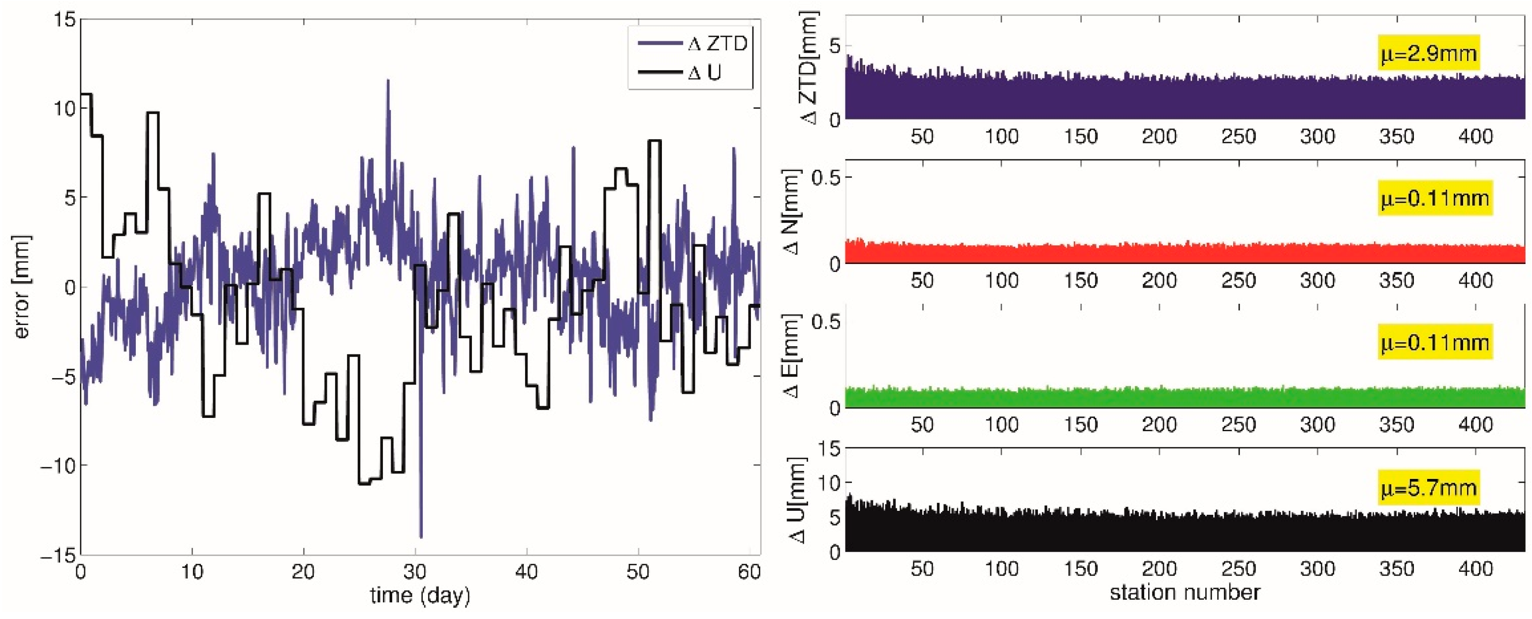
3.1. Experiment 1
3.2. Experiment 2
3.3. Experiment 3
3.4. Experiment 4
3.5. Experiment 5
4. Discussion
4.1. On the Relation between the Tropospheric Parameter Z0 and the Errors in the GNSS Estimates
4.2. Preliminary Results from GNSS Meteorology in Central Europe
5. Conclusions
- The quality of GNSS estimates is weather dependent. The reason being that the tropospheric delay model is inaccurate. This tropospheric delay model is based on a climatology or a NWM, and neither of these can be regarded as error free. The larger the deviation of the climatology or the NWM from the true state of the atmosphere, the larger the errors in the GNSS estimates. This is obvious and claimed in many studies; however, it is not trivial to provide some numbers. We provide such numbers. In essence, for the considered area and period, when the climatology was utilized in the tropospheric delay model, the error in the estimated ZTD and station up-component was about 2.9 mm and 5.7 mm, respectively. This error must be understood in a statistical sense; the individual errors can be roughly five times larger.
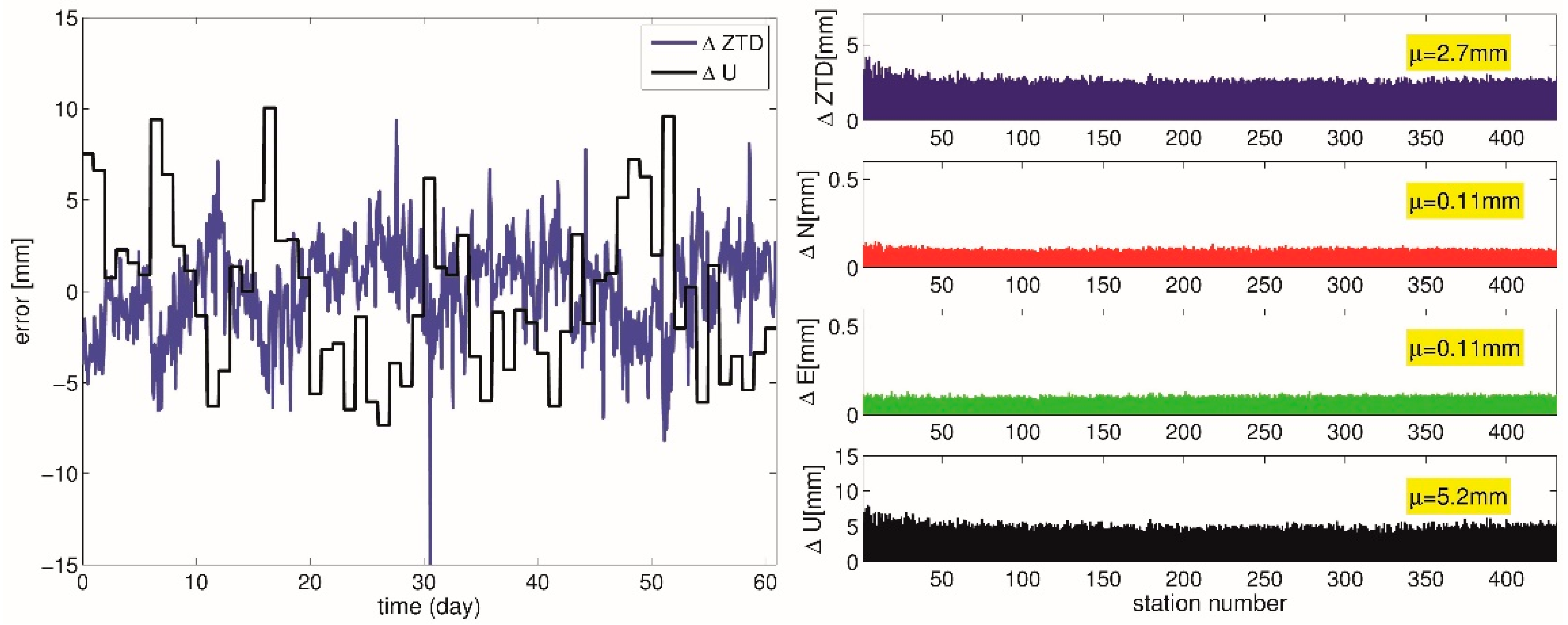
- The error in the GNSS estimates can be reduced significantly if the true ZHD and the true hydrostatic MF are utilized in the GNSS analysis; in this case the error in the estimated ZTD and station up-component will be reduced to about 2.0 mm and 2.9 mm respectively. The true ZHD and the true hydrostatic MF are unknown. However, there is good reason to believe that the ZHD and the hydrostatic MF from a NWM (analysis or short range forecast) are close to the true ZHD and the true hydrostatic MF. This also explains the success of the NWM based MFs that are currently recommended for analyzing space geodetic data [10]. An indication of the high quality of the NWMs in this respect is the agreement between them. For example, the two state of the art NWM based tropospheric delay models, VMF1 and UNB-VMF1, gave almost the same results in a geodetic analysis [14]. There were some differences for specific locations and times, but a clear advantage of one NWM over the other was not demonstrated in a statistical sense.
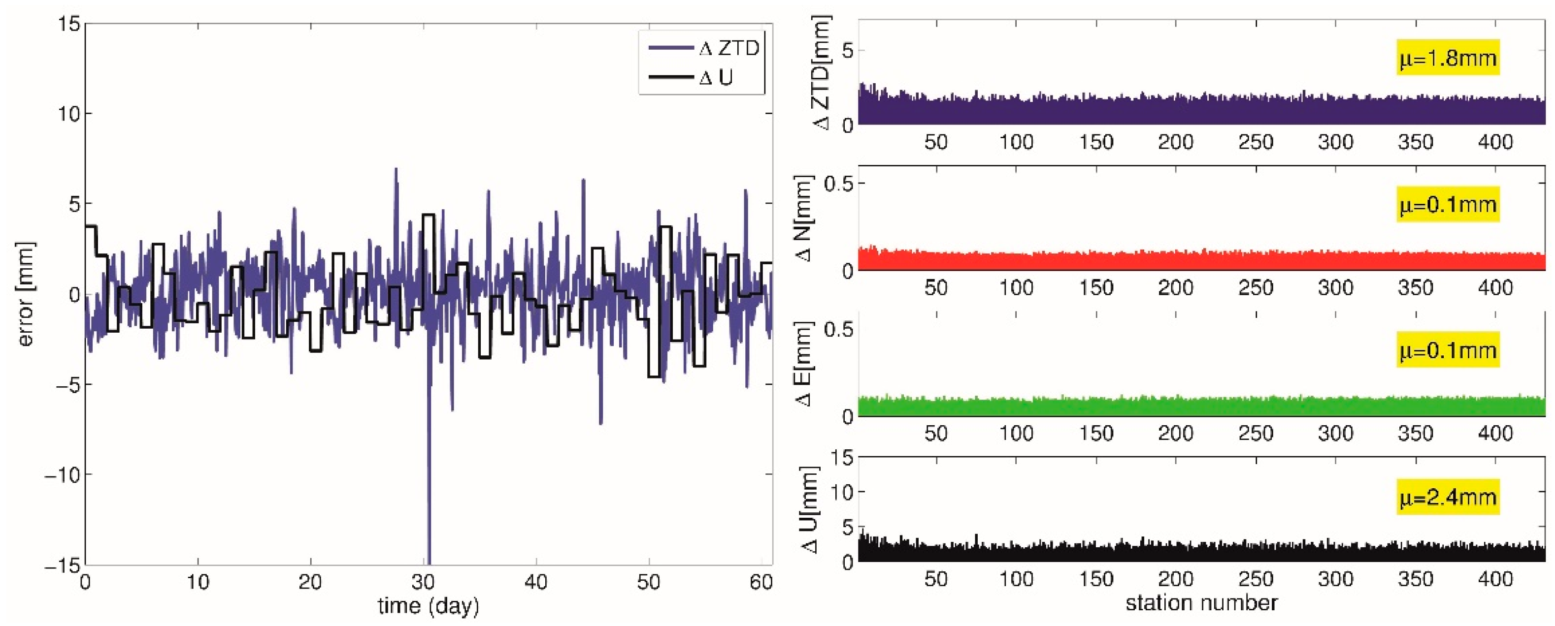
- The simulation study showed that the wet MF, when calculated under the assumption of a spherically layered troposphere, did not matter too much. In essence, when the true wet MF (calculated from the true refractivity profile above the station in question) is utilized in the GNSS analysis, the error in the estimated ZTD and station up-component remains about 1.8 mm and 2.4 mm, respectively. This is somewhat surprising; however, it is in line with the results from [9]. This study demonstrates that the improvement that may be realized for the wet MF is significantly less than for the hydrostatic MF. Reference [9] stated that: “… Contrary to the expectation that water vapor is the major source of error, the height error is dominated by the hydrostatic component, except possibly near the equator. Thus it is clear that an improvement in the hydrostatic component will have the larger impact on improving the measurement of height and atmosphere delay by VLBI and GPS”. However, the assumption is that the atmosphere is spherically layered. This brings us to the next item.
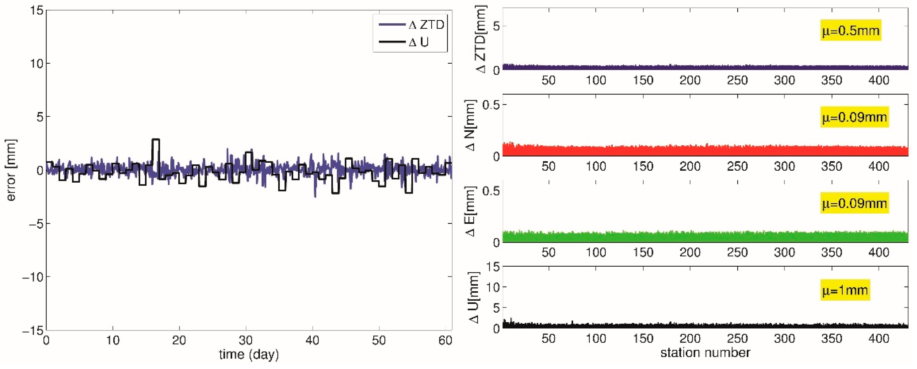
- We developed a modified wet MF, which is no longer based on the assumption of a spherically layered atmosphere. We have shown that with this modified wet MF the error in the estimated ZTD and station up-component can be reduced to about 0.5 mm and 1.0 mm, respectively. Its success, in practice, depends on the current (future) NWMs predicting the fourth coefficient of the developed closed form expression. We provided some evidence that current NWMs are able to do so. The determination of the modified wet MF is more expensive than the standard wet MF; the determination of the standard wet MF requires 10 tropospheric delays, whereas the determination of the modified wet MF requires an additional 120 tropospheric delays. The algorithm by [25], which calculates tropospheric delays with high speed and precision on an off-the-shelf PC also makes this feasible for real-time applications. We routinely calculate the additional 120 tropospheric delays, because they are required to determine the tropospheric gradients. The modified wet MF is a by-product of the simulation study (the primary purpose of our study was to quantify the tropospheric delay mismodelling). A more sophisticated MF concept could certainly be developed. In this respect, the newly developed VMF3 [15] sets a new standard, and we are going to analyze if we should follow this concept or refine our current concept in the future.
Author Contributions
Funding
Institutional Review Board Statement
Informed Consent Statement
Data Availability Statement
Acknowledgments
Conflicts of Interest
References
- Chen, G.; Herring, T.A. Effects of atmospheric azimuthal asymmetry on the analysis of space geodetic data. J. Geophys. Res. 1997, 102, 20489–20502. [Google Scholar] [CrossRef]
- Zumberge, J.F.; Heflin, M.B.; Jefferson, D.C.; Watkins, M.M.; Webb, F.H. Precise point positioning for the efficient and robust analysis of GPS data from large networks. J. Geophys. Res. 1997, 102, 5005–5017. [Google Scholar] [CrossRef] [Green Version]
- Bevis, M.; Businger, S.; Herring, T.A.; Rocken, C.; Anthes, R.A.; Ware, R. GPS meteorology: Remote sensing of atmospheric water vapor using the Global Positioning System. J. Geophys. Res. 1992, 97, 15787–15801. [Google Scholar] [CrossRef]
- Elosegui, P.; Davis, J.L.; Gradinarsky, L.P.; Elgered, G.; Johansson, J.M.; Tahmoush, D.A.; Rius, A. Sensing atmospheric structure using small-scale space geodetic networks. Geophys. Res. Lett. 1999, 26, 2445–2448. [Google Scholar] [CrossRef] [Green Version]
- Guerova, G.; Jones, J.; Douša, J.; Dick, G.; de Haan, S.; Pottiaux, E.; Bock, O.; Pacione, R.; Elgered, G.; Vedel, H.; et al. Review of the state of the art and future prospects of the ground-based GNSS meteorology in Europe. Atmos. Meas. Tech. 2016, 9, 5385–5406. [Google Scholar] [CrossRef] [Green Version]
- Tregoning, P.; Herring, T.A. Impact of a priori zenith hydrostatic delay errors on GPS estimates of station heights and zenith total delays. Geophys. Res. Lett. 2006, 33, L23303. [Google Scholar] [CrossRef] [Green Version]
- Boehm, J.; Heinkelmann, R.; Schuh, H. Short Note: A global model of pressure and temperature for geodetic applications. J. Geod. 2007, 81, 679–683. [Google Scholar] [CrossRef]
- Boehm, J.; Niell, A.; Tregoning, P.; Schuh, H. Global mapping function (GMF): A new empirical mapping function based on numerical weather model data. Geophys. Res. Lett. 2006, 33, 943–951. [Google Scholar] [CrossRef] [Green Version]
- Niell, A.E. Improved atmospheric mapping functions for VLBI and GPS. Earth Planet Space 2000, 52, 699–702. [Google Scholar] [CrossRef] [Green Version]
- Boehm, J.; Werl, B.; Schuh, H. Troposphere mapping functions for GPS and VLBI from European centre for medium-range weather forecasts operational analysis data. J. Geophys. Res. 2006, 111, B02406. [Google Scholar] [CrossRef]
- Lu, C.; Zus, F.; Ge, M.; Heinkelmann, R.; Dick, G.; Wickert, J.; Schuh, H. Tropospheric delay parameters from numerical weather models for multi-GNSS precise positioning. Atmos. Meas. Tech. 2016, 9, 5965–5973. [Google Scholar] [CrossRef] [Green Version]
- Balidakis, K.; Nilsson, T.; Zus, F.; Glaser, S.; Heinkelmann, R.; Deng, Z.; Schuh, H. Estimating integrated water vapor trends from VLBI, GPS, and numerical weather models: Sensitivity to tropospheric parameterization. J. Geophys. Res. Atmos. 2018, 123, 6356–6372. [Google Scholar] [CrossRef] [Green Version]
- Wilgan, K.; Hadas, T.; Hordyniec, P.; Bosy, J. Real-time precise point positioning augmented with high-resolution numerical weather prediction model. GPS Solut 2017, 21, 1341–1353. [Google Scholar] [CrossRef] [Green Version]
- Nikolaidou, T.; Balidakis, K.; Nievinski, F.G.; Santos, M.C.; Schuh, H. Impact of different NWM-derived mapping functions on VLBI and GPS analysis. Earth Planets Space 2018, 70, 95. [Google Scholar] [CrossRef] [Green Version]
- Landskron, D.; Böhm, J. VMF3/GPT3: Refined discrete and empirical troposphere mapping functions. J. Geod. 2018, 92, 349–360. [Google Scholar] [CrossRef]
- Zhou, Y.; Lou, Y.; Zhang, W.; Bai, J.; Zhang, Z. An improved tropospheric mapping function modeling method for space geodetic techniques. J. Geod. 2021, 95, 98. [Google Scholar] [CrossRef]
- Thayer, G.D. An improved equation for the radio refractive index of air. Radio Sci. 1974, 9, 803–807. [Google Scholar] [CrossRef]
- Skamarock, W.C.; Klemp, J.B.; Dudhia, J.; Gill, D.O.; Barker, D.M.; Duda, M.G.; Huang, X.Y.; Wang, W.; Powers, J.G. A Description of the Advanced Research WRF Version 3; NCAR tech. note NCAR/TN-475+STR; NCAR: Boulder, CO, USA, 2008. [Google Scholar] [CrossRef]
- Thompson, G.; Field, P.R.; Rasmussen, R.M.; Hall, W.D. Explicit Forecasts of Winter Precipitation Using an Improved Bulk Microphysics Scheme. Part II: Implementation of a New Snow Parameterization. Mon. Weather. Rev. 2008, 136, 5095–5115. [Google Scholar] [CrossRef]
- Kain, J.S. The Kain–Fritsch convective parameterization: An update. J. Appl. Meteorol. 2004, 43, 170–181. [Google Scholar] [CrossRef] [Green Version]
- Hong, S.Y.; Noh, Y.; Dudhia, J. A new vertical diffusion package with an explicit treatment of entrainment processes. Mon. Weather. Rev. 2006, 134, 2318–2341. [Google Scholar] [CrossRef] [Green Version]
- Iacono, M.J.; Delamere, J.S.; Mlawer, E.J.; Shephard, M.W.; Clough, S.A.; Collins, W.D. Radiative forcing by long–lived greenhouse gases: Calculations with the AER radiative transfer models. J. Geophys. Res. 2008, 113, D13103. [Google Scholar] [CrossRef]
- Tewri, M.; Chen, F.; Wang, W.; Dudhia, J.; LeMone, M.A.; Mitchell, K.; Ek, M.; Gayno, G.; Wegiel, J.; Cuenca, R.H. Implementation and verification of the unified NOAH land surface model in the WRF model. In Proceedings of the 20th Conference on Weather Analysis and Forecasting/16th Conference on Numerical Weather Prediction, Seattle, WA, USA, 12–16 January 2004; pp. 11–15. [Google Scholar]
- Jimenez, P.A.; Jimy Dudhia, J.; Gonzalez-Rouco, F.; Navarro, J.; Montavez, J.P.; Garcia-Bustamante, E. A revised scheme for the WRF surface layer formulation. Mon. Weather Rev. 2012, 140, 898–918. [Google Scholar] [CrossRef] [Green Version]
- Zus, F.; Bender, M.; Deng, Z.; Dick, G.; Heise, S.; Shang-Guan, M.; Wickert, J. A methodology to compute GPS slant total delays in a numerical weather model. Radio Sci. 2012, 47, RS2018. [Google Scholar] [CrossRef] [Green Version]
- Zus, F.; Dick, G.; Douša, J.; Heise, S.; Wickert, J. The rapid and precise computation of GPS slant total delays and mapping factors utilizing a numerical weather model. Radio Sci. 2014, 49, 207–216. [Google Scholar] [CrossRef]
- Zus, F.; Dick, G.; Heise, S.; Wickert, J. A forward operator and its adjoint for GPS slant total delays. Radio Sci. 2015, 50, 393–405. [Google Scholar] [CrossRef] [Green Version]
- Zus, F.; Douša, J.; Kačmařík, M.; Václavovic, P.; Dick, G.; Wickert, J. Estimating the Impact of Global Navigation Satellite System Horizontal Delay Gradients in Variational Data Assimilation. Remote Sens. 2019, 11, 41. [Google Scholar] [CrossRef] [Green Version]
- Niell, A.E. Global mapping functions for the atmosphere delay at radio wavelengths. J. Geophys. Res. 1996, 101, 3227–3246. [Google Scholar] [CrossRef]
- Santos, M.C.; McAdam, M.; Böhm, J. Implementation status of the UNB-VMF1. In Proceedings of the European Geosciences Union General Assembly 2012, Vienna, Austria, 22–27 April 2012. [Google Scholar]
- Zus, F.; Dick, G.; Dousa, J.; Wickert, J. Systematic errors of mapping functions which are based on the VMF1 concept. GPS Solut. 2015, 19, 277. [Google Scholar] [CrossRef]
- King, M.A.; Watson, C.S. Long GPS coordinate time series: Multipath and geometry effects. J. Geophys. Res. 2010, 115, B04403. [Google Scholar] [CrossRef]
- Zus, F.; Deng, Z.; Wickert, J. The impact of higher-order ionospheric effects on estimated tropospheric parameters in Precise Point Positioning. Radio Sci. 2017, 52, 963–971. [Google Scholar] [CrossRef] [Green Version]
- Davis, J.L.; Herring, T.A.; Shapiro, I.I.; Rogers, A.E.E.; Elgered, G. Geodesy by radio interferometry: Effects of atmospheric modeling errors on estimates of baseline length. Radio Sci. 1985, 20, 1593–1607. [Google Scholar] [CrossRef]
- Douša, J.; Dick, G.; Kačmařík, M.; Brožková, R.; Zus, F.; Brenot, H.; Stoycheva, A.; Möller, G.; Kaplon, J. Benchmark campaign and case study episode in central Europe for development and assessment of advanced GNSS tropospheric models and products. Atmos. Meas. Tech. 2016, 9, 2989–3008. [Google Scholar] [CrossRef] [Green Version]
- Landskron, D.; Böhm, J. Refined discrete and empirical horizontal gradients in VLBI analysis. J. Geod. 2018, 92, 1387–1399. [Google Scholar] [CrossRef] [PubMed] [Green Version]
- Dick, G.; Gendt, G.; Reigber, C. First Experience with Near Real-Time Water Vapor Estimation in a German GPS Network. J. Atmos. Sol.-Terr. Phys. 2001, 63, 1295–1304. [Google Scholar] [CrossRef]
- Gendt, G.; Dick, G.; Reigber, C.; Tomassini, M.; Lui, Y.; Ramatschi, M. Near real time GPS water vapor monitoring for numerical weather prediction in Germany. J. Meteorol. Soc. Jpn. 2004, 82, 361–370. [Google Scholar] [CrossRef] [Green Version]


| Experiment | ZHD | mh | mw |
|---|---|---|---|
| #1 | GPT | GMFh | GMFw |
| #2 | NWM | GMFh | GMFw |
| #3 | NWM | PMFh | GMFw |
| #4 | NWM | PMFh | PMFw |
| #5 | NWM | PMFh | PMFz |
Publisher’s Note: MDPI stays neutral with regard to jurisdictional claims in published maps and institutional affiliations. |
© 2021 by the authors. Licensee MDPI, Basel, Switzerland. This article is an open access article distributed under the terms and conditions of the Creative Commons Attribution (CC BY) license (https://creativecommons.org/licenses/by/4.0/).
Share and Cite
Zus, F.; Balidakis, K.; Dick, G.; Wilgan, K.; Wickert, J. Impact of Tropospheric Mismodelling in GNSS Precise Point Positioning: A Simulation Study Utilizing Ray-Traced Tropospheric Delays from a High-Resolution NWM. Remote Sens. 2021, 13, 3944. https://doi.org/10.3390/rs13193944
Zus F, Balidakis K, Dick G, Wilgan K, Wickert J. Impact of Tropospheric Mismodelling in GNSS Precise Point Positioning: A Simulation Study Utilizing Ray-Traced Tropospheric Delays from a High-Resolution NWM. Remote Sensing. 2021; 13(19):3944. https://doi.org/10.3390/rs13193944
Chicago/Turabian StyleZus, Florian, Kyriakos Balidakis, Galina Dick, Karina Wilgan, and Jens Wickert. 2021. "Impact of Tropospheric Mismodelling in GNSS Precise Point Positioning: A Simulation Study Utilizing Ray-Traced Tropospheric Delays from a High-Resolution NWM" Remote Sensing 13, no. 19: 3944. https://doi.org/10.3390/rs13193944