1. Introduction
The Global Navigation Satellite System—Continuously Operating Reference Station (GNSS -CORS) network stations that are designed with excellent spatial density and distribution are used for various geodetic and non-geodetic applications [
1,
2,
3,
4,
5]. The estimation of seasonal changes of CORS positions plays an extremely important role, since it can impact the final estimates, particularly the site velocity [
6,
7,
8]. Three key categories can be defined in terms of potential contributors to the seasonal variation observed at CORS sites. Included in the first category are the influence of the gravitational excitation, primarily from the Sun and Moon, universal time corrected for polar motion (UT1—Universal Time) variation, rotational displacements due to the seasonal polar motion, loading-induced displacements due to solid Earth tides, ocean tides and the effects of atmospheric tides [
9,
10,
11]. Pole tides with a predominantly annual spectrum and Chandler wobble periods are also included in this category [
9]. The second category of seasonal variation contains the thermal origin coupled with hydrodynamics [
12]. The seasonal deformation induced by loadings from non-tidal sea surface fluctuation, atmospheric pressure and groundwater (in a solid or liquid state) is included in this second category [
13]. An additional perturbation that belongs to this category is the thermal expansion of bedrock beneath the GNSS site and the wind shear which can induce site displacements. The third category is a conglomerate of various errors that generate apparent seasonal variation, such as water vapour distribution models, satellite orbital models, antenna thermal noise, phase centre variation models, atmospheric models, local multipath and snow cover on the antenna (which could be the source of the apparent variation in the estimated site position) [
9,
14].
The parameters and associated error for the CORS coordinates time series (computed from GNSS measurements) were estimated using the maximum likelihood estimation (MLE) method [
15,
16,
17]. For their analysis, seasonal signals are modelled as sinusoids with annual and semi-annual harmonics that are commonly modelled by two periodic signals, each with constant amplitude and phase-lag [
18,
19,
20]. The seasonal signal includes power at all annual harmonic frequencies which will affect the time domain and spectral characterisation of point coordinates determined from GNSS measurements [
6]. The surface loading, particularly due to the hydrology and atmospheric pressure, is the primary cause for the annual signal with respect to a global reference frame. The loading models of continental water storage reports according to van Dam et al. [
21] reported that ‘
a vertical displacement of the CORS positions has root mean square (RMS) values as large as 8 mm and are predominantly annual in character’. The seasonal variation is best described by a deterministic model rather than a power-law noise model and it makes a significant contribution to the velocity error for global and regional reference CORS stations, determined by using GNSS, especially over a short data span.
In a time series of analysed data, the widely used ‘standard deviation’ does not allow for noise and drifts to be distinguished. Standard deviation is a very general characteristics of the noise level in the time series. In addition, it is affected by, e.g., outliers and trends (low-frequency position variations). Allan variance is practically free of these factors and additionally allows us to investigate the spectral characteristics of the time series, such as noise type, which is important for understanding the physical origin of the observed geodetic signal. Moreover, standard deviation changes with the increase number of samples and tells only where the majority of the data lie, while Allan variance (AVAR) gives an information about values in specific distances between data (τ-averaging time). On the other hand, AVAR as a time-domain statistic is used for a variety of sensors and discrete data measurements, e.g., gyroscopes, microwave radiometers and many others [
22,
23,
24,
25]. Its Allan deviation (ADEV), the square root of the AVAR, provides magnitude versus time separation in a log–log plot that allows for simple detection of various noise and drift types, which can be identified by the slopes for different plot regions [
26,
27]. ADEV also provides a measure that avoids the issue of divergence of the typical standard deviation as the number of measurement samples is increased in the presence of flicker noise and drift, along with the associated inability to precisely define the time average of the measurement [
28,
29]. To date, ADEV has been used to a limited extent in the GNSS positioning error time series through only a few studies. Niu et al. [
30] analysed the GNSS positioning error characterised through the usage of AVAR in three different modes: Differential Global Positioning System (DGPS), GPS and PPP (Precise Point Positioning). Four different types of noise were observed: 1st order Gauss–Markov process, white noise, random walk noise and flicker noise. The principal conclusion of the study is that white noise is not always an optimal model for the GNSS positioning time series, and it does not describe the majority of changes in the analysed coordinates time series. In another study, AVAR was utilised to improve the overall performance of microelectromechanical systems (MEMS)-based inertial navigation system (INS) error models for modelling inertial sensor errors instead of the commonly recommended auto-regressive processes [
31].
ADEV is used for other processes besides clock performance, for instance, its modified versions, e.g., Hadamard deviation (HDEV) or modified ADEV, which facilitate noise characteristics that are less sensitive to outliers than the original ADEV [
32]. The MLE method allows for the detection of all noise [
33]. Reference [
34] came to the conclusion that the white noise is not dominant in a GNSS time series analysis, and the characteristics of the stations can be properly described by a white noise plus flicker noise model. In this study, 3 years of daily, globally distributed CORS sites were analysed, and all components were modelled using a combination of white noise plus flicker noise. Williams [
35] analysed continuous time series of 414 individual CORS sites, and the results showed a combination of white noise and flicker noise, while random walk noise amplitudes were several times smaller than the white noise and flicker noise. Hackl et al. [
36] estimated velocity uncertainties from CORS error time series affected by time-correlated noise. Most of the analysed time series of the South African TrigNet network were modelled using power-law noise plus annual signals. Rate uncertainty with MLE was conducted by Langbein [
37], and the results suggested that long-period noise is best characterised by flicker noise or power-law noise. Moreover, multiple long time series of CORS data suggest that the random walk component was not presented. Similarly, CORS time series from south Asia were analysed by Ray et al. [
38] using the MLE method, and the results demonstrated that most of the analysed data were characterised by a combination of either white noise plus flicker noise or white noise plus random walk noise.
To obtain information on the frequency and its localisation in time, spectral analysis methods such as fast Fourier transformation (FFT) is commonly used in various fields of science and engineering [
39]. Such time-frequency analysis is used for studies of non-stationary processes such as seismic events; meteorological phenomena or pattern recognition, denoising, prediction and filtering. Another method of time-frequency analysis is to use a wavelet transform, which is particularly useful in studies of signal stationarity [
40].
During the past two decades, significant geophysical phenomena and associated studies that made use of high-rate GNSS data, at 1 to 20 Hz, for CORS position determination have been conducted across Europe [
41]. This led to the analysis of slow deformation processes and fast geophysical phenomena such as crustal earthquakes [
42], landslides and magma injection. Numerous studies have focused on coseismal displacement waveforms for the 24 August 2016 6.2 M
w Amatrice earthquake (central Italy) obtained from high-rate GPS data [
43] and the 2009 L’Aquila earthquake [
44]. Moreover, monitoring of earthquakes; active landslides in Italy [
45], Croatia and Portugal; coal mine subduction areas in Hungary and Romania [
46] and active volcanos in Italy, Iceland [
47] and the Azores facilitates a greater perspective of the predominant geophysical phenomena in Europe. All the significant geophysical phenomena that have occurred in Europe during the past two decades have had a strong local impact, except for the 2010 volcanic eruptions of Eyjafjallajökull (Iceland) when a cloud of ash covered a large section of the Northern Hemisphere.
Several research approaches with specific objectives are presented in this article. First, the wavelet transform is used to analyse CORS time series variations containing numerous frequency components, which allows for the identification of their variability over time. A continuous wavelet transform (CWT) is used for time series stationarity analysis. A comprehensive description of the application of the wavelet transform in geophysics can be found in [
48,
49]. Second, OHVAR (overlapping Hadamard variance) was employed to provide improved confidence compared to AVAR, which is typically used for the determination of noise types specific to a particular averaging time. To obtain the residuals, we subtracted the fitted linear trend by using Least Square Estimation (LSE) on the raw data, from the observations. The residuals were then ordered by size, and the interquartile range was computed. The residuals with a value less than 3 times the interquartile range (IQR) below or above the median was considered an outlier [
50]. Based on this ‘cleaning’ method, we have obtained the ‘clean’ data, from which we have computed the annual and semi-annual seasonal signals. The third and final objective was to analyse the impact of three different types of geophysical events, such as earthquakes with a magnitude greater than 6° on the Richter scale, landslides, and volcanic activity on the amplitude and variation of the seasonal signal. The analysed GNSS time series was divided as a function of geophysical event—the data with time span that contains the geophysical events, before and after the geophysical event. Regarding the earthquake events, the seasonal signal was computed with different time spans as a function of the time of the geophysical event, but also at various radii from the epicentre of the earthquake such as 30, 60 and 100 km.
2. Data and Analysis Methods
The authors analysed the daily GPS-based PPP results of 196 CORS stations from the EUREF-Permanent Network (EPN) network over 25 years (from 1 January 1995 to 31 December 2009). The location of these stations will be shown, for example, in
Figure 1. For newer stations within the network, at least 10 years of continuous data were included (as of 31 December 2019). Daily PPP solutions for the 196 EPN stations were obtained from the Nevada Geodetic Laboratory (NGL). The parameters used in PPP processing were provided by Blewitt et al. [
51]. The topocentric components of the stations were next analysed following the methodology discussed below.
For the performed GNSS-based CORS coordinate time series analysis, parameters like linear trend, seasonal signal and noise and their associated errors are estimated using the MLE method [
14,
15,
33]. In general, the seasonal signal is modelled as sinusoidal with annual and semi-annual harmonics that are commonly demonstrated by two periodic signals, each with a constant amplitude. The power spectrum
that describes many types of physical and geophysical processes whose behaviour in the time domain denoted by [
52,
53] is
where
is the spatial or temporal frequency,
and
are normalising constants, and
is a spectral index. Typically, the spectral index
lies within the range −3 to 1 [
53]. The process within this range is subdivided into ‘fractional Brownian motion’ with
and ‘fractional white noise’ or ‘fractional Gaussian’, which is a stationary process with
, including the special case of uncorrelated white noise, with
, and
is flat [
54,
55]. Within such stochastic models, special cases occur. For example, at
(or
) flicker noise occurs, and at
(or
) Brownian motion takes place (the so-called ‘random walk’). The term ‘coloured noise’ is used to refer to power-law processes that differ from classical white noise.
With reference to [
56,
57], in order to estimate the parameters that describe the trend and noise in the GNSS observations we must maximise the probability
for given observations
, such as the CORS point coordinates analysed in this study. If a Gaussian distribution is assumed, then this probability is expressed as
where
denotes the determinant of the matrix;
represents the covariance matrix of the assumed noise in the data;
N is the number of epochs;
are the post-fit residuals of the linear function using weighted least squares with the same covariance matrix
, expressed as
where the vector
contains the parameters for the nominal value which is the offset of the entire time series and the trend. The observation matrix
has
rows and 2 columns. The first contains solely ones, and the second column contains the linear trend. Langbein noted that it is straightforward to also include a yearly signal and offsets in the estimation process [
16]. Hence, the observed trend reduced by the estimated trend will produce the residuals
.
In practice, the maximum of the logarithm of this probability
is computed, which is an equivalent issue because the logarithm is a monotonically increasing function. The covariance matrix,
depends on the noise and not on
. Therefore, the maximum probability can be found by setting the derivative of the logarithm of Equation (2) to zero, such that
This represents the weighted least squares solution. In terms of stability, the logarithm of the likelihood must be maximised, where
since the maximum is unaffected by the monotonic transformation.
Another analysis tool is AVAR and its modifications. AVAR is used to intercompare time series and their internal noise through the calculation of the deviation for a discrete set of different averaging times (
τ). There are many variations of AVAR, e.g., modified AVAR (MVAR), overlapping AVAR (OVAR) or Hadamard variation (HVR), which allow for additional noise types to be distinguished. Moreover, overlapped variations provide better confidence than non-overlapped variations but require greater computational time. In this study, we used overlapping HVAR (OHVAR). This type of variance is estimated from the set of
fractional frequency measurements
for the averaging time
, where
is the averaging factor (usually consecutive powers of 2 or 10), and
is the basic measurement interval, expressed by [
58].
There are many variations of AVAR, e.g., modified AVAR (MVAR), overlapping AVAR (OVAR) or Hadamard variation (HVR), which allow for additional noise types to be distinguished. Moreover, overlapped variations provide better confidence than non-overlapped variations but require greater computational time. In this study, we used overlapping HVAR (OHVAR). This type of variance is estimated from the set of
fractional frequency measurements
for the averaging time
, where
is the averaging factor (usually consecutive powers of 2 or 10), and
is the basic measurement interval, expressed by [
58]:
where,
is the
ith of
fractional frequency values at each measurement time. In terms of the GNSS data (North, East and Up components), a set of
time measurements of MVAR is defined as
for measurement time. The results are generally expressed as the square root,
, i.e., the OHDEV. Based on an analysis of the literature, the OHVAR method was chosen (due to improved confidence compared to the AVAR) to mitigate divergent noise and infer the noise components in the GPS data [
59].
Periodic changes of CORS station coordinates are often non-stationary (i.e., in the sense that they have variable instantaneous amplitude and frequency), and higher harmonic components may be present. These effects can be caused by varying environmental conditions in the vicinity of the antenna, the changing of measurement equipment at the station (replacement of the receiver or antenna), or variations of a geodynamic nature. To verify the stationarity and identify the nature of signal changes, a time-frequency analysis was performed using CWT. The Morlet wavelet was adopted as the mother wavelet. This kind of wavelet is commonly used in the analysis of geophysical phenomena and provides results with equal variance in time and frequency domains [
49]. CWT allows for the examined signal to be presented in the form of a scalogram—a time-frequency spectrum, which allows for the identification of both frequencies present in the signal and their location in time. CWT is defined as a convolution of the analysed signal
s(
t) with scaled and shifted wavelet function
ψ(
t) [
60]:
where
represents the scale;
denotes the translation;
represents the mother wavelet;
* denotes the complex conjugate.
The normalisation factor
is used to preserve direct comparability of the transform for all scales. The Morlet wavelet used here to calculate the time-frequency spectrum is expressed as
where
The continuous wavelet transform method does not optimize the time and frequency resolution simultaneously. In CWT analysis, a trade-off must be found between these quantities [
61]. In the present study, the centre frequency was taken as
f = 1.2 Hz, and the bandwidth parameter
fb = 2.0 for all the coordinate time series analysed. The parameter values were selected empirically to ensure a balance between the time and frequency resolution satisfactory for analysed data.
3. Results
To obtain reliable estimates of the seasonal terms and as mentioned earlier, CORS stations that had at least GNSS observations span of greater than 10 years (December 2009–December 2019) were included. The time series that were analysed in terms of seasonal variation consisted of data cleaned from outliers by fitting a linear trend to the raw data using the Least Square Estimation (LSE) technique and by subtracting this linear trend from the observations to obtain the residuals. The residuals were ordered by size and the IQR is computed—these values represented the difference between the sorted array of the values of the residuals at 75% and the values of the residuals at 25%. Any residual with a value greater than 3 times the IQR, below or above the median, was considered to be an outlier [
50,
62]. The annual and semi-annual seasonal signals were included during pre-processing to obtain clean data. The daily time series were pre-processed not only for outliers but also for offsets and gaps and were analysed with the help of MLE computed by the use of Hector software package [
62]. Although the gaps were determined, no interpolation technique was used before estimating the parameters. The epochs of the offsets (caused, in general, by technical operations for, e.g., antenna changes) were obtained directly from the log files of the stations and/or by inspection of the time series to identify offsets from unknown origin. Spectral analysis was performed on all stations using the Lomb–Scargle algorithm since interpolation of the unevenly spaced data is not required [
63,
64].
The following sub-sections will present and discuss the results of seasonal amplitudes, the impact of geophysical events on seasonal signal, overlapping Hadamard variation and finally the time-frequency results.
3.1. Seasonal Amplitudes
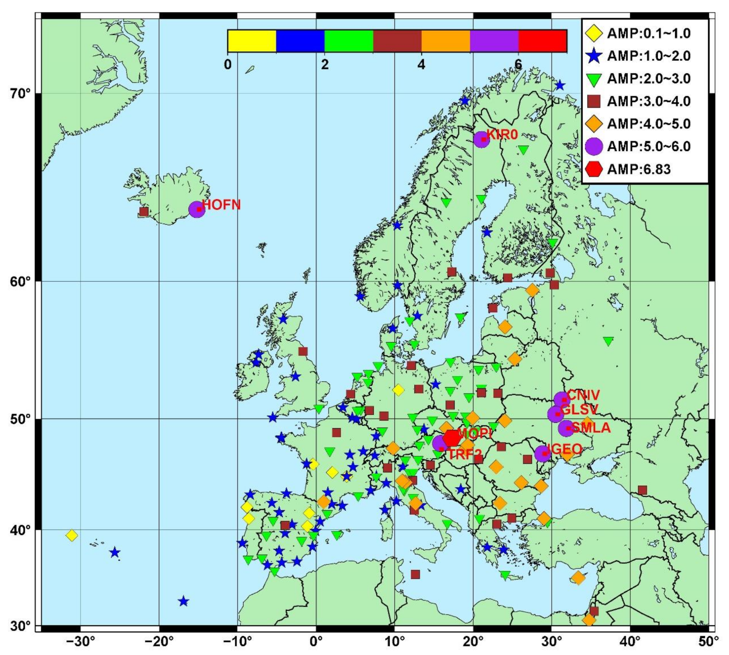
Figure 1 presents the seasonal amplitude of (a) East component and (b) North component for all the analysed stations. The names of the stations with the higher values of seasonal amplitude are showed with red colour.
Starting from the East component, the minimum and maximum of yearly seasonal amplitudes are 0.114 mm and 6.049 mm, with a median value of 0.817 mm. The minimum and maximum semi-annual seasonal amplitude are 0.088 mm and 1.114 mm, with a median value of 0.272 mm. Roughly, 62% of the stations located in mainland Europe experience seasonal yearly amplitude between 0.1 mm and 1.0 mm. There are five stations that are considered as exceptions with an amplitude between 2.0 mm and 3.0 mm; these are the ESCO, SMLA and TORI CORS stations located in mainland Europe, which have amplitudes of 2.01 mm, 2.51 mm and 2.41 mm with formal errors of 0.10 mm, 0.24 mm and 0.12 mm, respectively. The other two stations are located at the edge of Iceland—the REYK and HOFN stations—both with the same amplitudes of 2.03 mm with formal errors of 0.12 mm and 0.15 mm, respectively. The largest amplitudes of 3.20 mm and 6.049 mm were experienced at the BOLG stations situated in Italy and the CAKO station situated in Croatia (shown as a red polygon), with formal errors of 0.17 mm and 0.211 mm, respectively.
The amplitude for the North component is shown in
Figure 1. The minimum and maximum yearly seasonal amplitudes were 0.132 mm and 4.587 mm, respectively, with a median value of 0.651 mm. The semi-annual seasonal amplitudes were 0.105 mm and 0.968 mm, with a median value of 0.266 mm. The maximum North seasonal influence and daily coordinate variation were observed for station SMLA (Ukraine), shown as a red polygon.
Figure 2 illustrates the amplitude measurements for the Up component. The minimum and maximum yearly seasonal amplitudes were 0.443 mm and 6.833 mm, respectively, with a median value of 2.448 mm. The semi-annual seasonal amplitudes were 0.299 mm and 2.936 mm, with a median value of 0.712 mm. The vertical (up) annual amplitudes were less than 7 mm and most of the stations from mainland Europe had amplitudes between 1.0 mm and 5.0 mm with a corresponding formal error of less than 0.8 mm.
Only eight stations had a seasonal amplitude of less than 1.0 mm. The two stations located in Iceland (REYK and HOFN) experienced amplitudes of 3.19 mm and 5.44 mm, with formal errors less than 0.5 mm. Station MOPI (Slovakia, shown as a red polygon) had highest and interesting results, which will be discussed in the following sub-section.
3.2. Analysis of the Impact of Geophysical Events on Seasonal Signals
In addition to the results presented in previous figures, a subset of several geophysical events, which occurred between 2000 and 2020, were selected to assess their impact on the seasonal signal. These events included earthquakes with a magnitude greater than 6° on the Richter scale, landslides and volcanic activity which are presented in
Figure 3.
Several of the events presented in
Figure 3. were further analysed by grouping the CORS stations determined by GNSS as a function of the radius from the geophysical event—from 0 km to 100 km and considering the stations identified within those radiuses, which are presented in
Table 1.
The main objective of the analysis in this section is to compare the seasonal signal for the CORS station that contains the geophysical events with the timespan before and after the geophysical event. Therefore, to assess the impact of the geophysical events outlined in
Table 1, four computational strategies were selected:
- (a)
Seasonal signal values were computed by taking into account the entire length of the time series; this strategy was called ‘all the data’;
- (b)
The seasonal signal values were computed based on the four years of data prior to the geophysical event, up to the beginning of the year when the geophysical event occurred; this strategy was called ‘before the event’;
- (c)
The seasonal signal values were computed based on three years of data, in which the year when the geophysical event occurred was in the middle of the timespan; this strategy was named ‘during the event’;
- (d)
The seasonal signal values were computed based on the four years of data after the geophysical event, beginning from the year after the geophysical event occurred; this strategy was named ‘after the event’.
According to these strategies, the time series was split into three segments that overlapped with each other on one year of data. The CORS stations AQUI, REYK, UNPG and UNTR were subjected to two geophysical events; thus, they were also defined with numbers based on the time each event occurred, for example, station AQUI was named “AQUI-1” which only include the first event in 4 June 2009, and “AQUI-2” is station AQUI which contains only the group of events from 2016. The results are discussed for each of the position components (EAST, North and UP).
3.2.1. The East Component
The seasonal signal values for the East component, based on the four computational strategies mentioned above for the different geophysical events considered, are presented in
Figure 4. The station AQUI-1 which is located within a radius of 30 km from an earthquake and stations UNPG-1 and UNTR-1 that were within 100 km from the earthquake showed a higher seasonal signal value when the data span included the geophysical event. For the landslide events, the stations MSRU, ROVE, VLSG and ZIMM showed higher seasonal signal values during the segment that included the event and for the volcanic activity; the stations LICO and REYK-2 showed higher seasonal signal values when the data span included the event.
Of the three stations that were within a radius of 30 km from an earthquake, only station AQUI had a higher seasonal signal value during the geophysical event timespan compared with the timespan before and after the geophysical event. For the landslide events, the stations MSRU and VLSG, which were within a radius of 30 km, had higher seasonal signal values during the geophysical event when comparing with the timespan before and after the geophysical episode. In the case of volcanic activity, only the stations LICO and FRUL experienced higher seasonal signal values. Of the five reference stations within a 60 km radius from an earthquake event, one station (MOPS) had a higher seasonal signal value. When a radius of 100 km was considered, the stations UNPG-1 and UNTR-1 had higher seasonal signal values (out of six stations). Moreover, one of two stations (ZIMM) had a higher seasonal signal value during the processed timespan which included the geophysical event. For volcanic activity, station REYK-2 had a higher seasonal signal value during the timespan that included the event.
3.2.2. The North Component
The seasonal signal values for the North component are presented in
Figure 5. Station AQUI-1 showed a higher seasonal signal value during the earthquake event timespan (
Figure 5). The other CORS stations that exhibited higher seasonal signal values were KITH and TIRA, which are located within 30 km radius from the event, stations BOLG, REYK-1, SHK0 which are in a radius of 60 km and stations UNPG-1 and UNTR-1, which are located in a radius of 100 km from the event. For the landslide events, the stations COMO, MSRU, ROVE and ZIMM had higher seasonal signal values when the computation included the event in the timespan. In the case of volcanic activity, the CORS stations ENAV, FRUL and REYK-2 experienced higher seasonal signal values during the period that included the event.
In the case of an earthquake event, all three stations within a radius of 30 km from the earthquake had higher North component seasonal signal values when the geophysical event was included during processing. For landslide events, station MSRU had a higher seasonal signal value during the timespan that included the event, whereas the seasonal signal values during and after the event for station VLSG were extremely similar. Concerning the effect of volcanic activity on the seasonal signal value, one of the five stations (ENAV) experienced a higher seasonal signal value when the event was considered during the processed timespan. However, the seasonal signal values for stations ENAV, ISCH and LICO, for all four computational strategies, had similar results. In the case of earthquakes, three of the five stations (BOLG, SHK0 and REYK-1) within a 60 km radius from the geophysical event exhibited higher seasonal signal values during the timespan that included the event. The two additional stations (MOPS and MSEL) had higher seasonal signal values before the geophysical event occurred. When a 100 km radius was considered in the case of earthquakes, two of the six stations (UNPG-1 and UNTR-1) had higher seasonal signal values during the timespan that included the event. In the case of landslides, all three CORS stations (COMO, ROVE and ZIMM) had higher seasonal signal values during the period that included the event, whereas, in the case of volcanic activity, only the station REYK-2 showed a higher seasonal signal value during the period that included the event.
3.2.3. The UP Component
The seasonal signal values for the Up component are presented in
Figure 5. Station AQUI-1 exhibited higher seasonal signal values when it was computed during the geophysical event (
Figure 6). A higher seasonal signal value for the Up component was also observed for the stations BOLG, MOPS, MSEL, SHK0, which are located within a radius of 60 km from the epicentre of the earthquake, but also stations AQUI-2, GARI and TUC2, which are within a radius of 100 km. In the case of landslide events, the seasonal signal values for the stations MSRU, VLSG and ROVE were also higher when the timespan included the event. The first two stations (MSRU and VLSG) were within a radius of 30 km from the event, whereas the third station (ROVE) was within a radius of 100 km from the event. For volcanic activity, the stations ENAV, FRUL, IPRO and LICO had higher seasonal signal values when the event was included in the timespan.
Within a radius of 30 km from an earthquake, the two additional stations (KITH and TIRA) showed higher seasonal signal values when all the data from the time series were considered before the geophysical event occurred. For landslides, both stations (MSRU and VLSG) had a higher seasonal signal value during the period that included the event, whereas, for volcanic activity, four of the five stations (IPRO, LICO, FRUL and ENAV) had higher seasonal signal values in the time series when the geophysical event was considered. The fifth station (ISCH) experienced a higher seasonal signal value before the geophysical event occurred. In the case of earthquakes, four of five stations within a 60 km radius (SHK0, MOPS, BOLG and MSEL) exhibited higher seasonal signal values when the geophysical event was included in the timespan. A higher seasonal value was observed for station REYK-1 when the entire time series was considered. For stations within a 100 km radius of earthquake events, three showed higher seasonal signal values when the event was included in the analysed timespan (AQUI-2, TUC2 and GARI); however, the GARI station experienced the same seasonal signal value in the period before the geophysical event occurred. For landslides, ROVE was the only station which showed a higher seasonal signal value when the geophysical event was included in the analysed timespan. In the case of volcanic activity, the REYK-2 CORS station exhibited a higher seasonal value during the period after the geophysical event occurred.
It can be seen that for the horizontal component, especially the North component, is more susceptible to geophysical events, which has more sites with higher amplitude when the geophysical event was accounted during the processed timespan. The same number of stations with higher seasonal amplitude during the geophysical event was observed also on the Up component.
3.3. Overlapping Hadamard Variation
This subsection contains noise stability analysis of the daily point coordinates based on the 15 years of continuous GNSS observations at the 196 CORS stations. The OHVAR and coordinate component were calculated for each station. The entire period analysed was divided into three 5-year parts (intervals): 1995–1999 (70 stations were established during this period), 2000–2004 (58 more stations) and 2005–2009 (additional 68 stations), as illustrated in
Figure 7. The above-mentioned years denote the deployment periods for each of the stations. The oldest stations were established at the end of 1995, resulting in approximately 25 years of continuous observations (approximately 8800 days) up to the year 2020. These analyses were made to compare if there is a time specific noises related to the period of the inclusion station into EPN on the other side—time of the operation. Comparing periods for the East (
Figure 7a–c) and North (
Figure 7d–f) components, there are very small differences in the stabilities on each graph of the analysed time series. It means that for the longest averaging time (512 days) differences between extreme stabilities (the smallest and the highest) are smaller for the 2005–2009 (
Figure 7c,f) year stations inclusion then for two other periods (1995–1999—
Figure 7a,d and 2000–2004—
Figure 7b,e). In case of the Up component, the situation is quite different—for the first period (
Figure 7g), for the longest averaging times (512 days), the differences between biggest and smallest stabilities are smaller than the right column for Up component (2005–2009 years,
Figure 7i).
Figure 8 shows the mean curves of each interval and component presented in
Figure 7. Firstly, no significant differences were observed between each period analysed. Additionally, the North (
Figure 8, green curve) and East (
Figure 8, blue curve) components were similar for the period of 1 to 100 days. For an averaging time (τ) greater than 100 days, these components differed slightly.
Moreover, above figure allows for determination noise type based on the slope of the curves between each averaging times. Analysing averaging time between 1 to 30 days, for the time interval 1995–1999, the East and North component power-law curve slopes were −0.335 and −0.356, respectively, which corresponds to flicker noise. In the case of the Up component, the value was −0.224, which also indicated the same noise. For the two other time intervals (2000–2004 and 2005–2009), the conclusions were mostly the same. In the case of 1 to 30 days, the τ for the first interval power law curve slopes were −0.264, −0.282 and −0.236 for the East, North and Up components, respectively. For the other intervals, the conclusions for the period of 1 to 30 days were similar and indicated flicker noise. For each interval of approximately 100 days of averaging time, a sinusoidal slope of the curve was visible. For a τ greater than of approximately 105 days, the slopes for each interval and coordinate component became random walk noise; however, the slopes were slightly different when the intervals between them were compared.
3.4. Time–Frequency Analysis
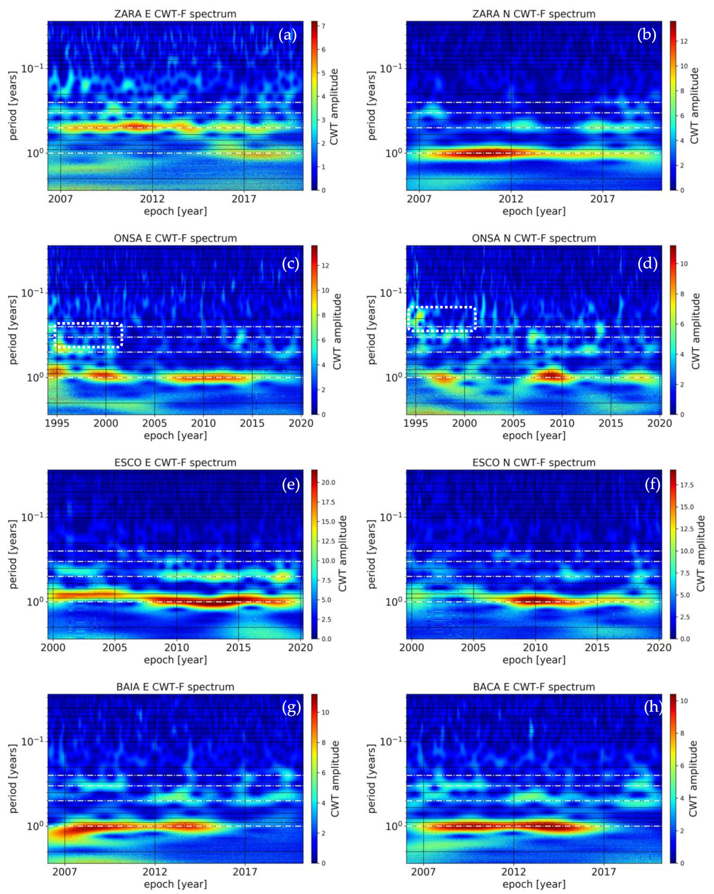
The time–frequency analysis of CORS station coordinate time series allowed for the identification of the dominant periodic components and their changes during the time span analysed. Time–frequency analysis was performed separately for each station and each coordinate. Special attention was given to the occurrence of a seasonal component (tropical year) and its higher harmonics. In most cases, the annual component was clearly visible. In a few analysed time series, dominant higher harmonics were observed.
Figure 9 shows several representative examples of the time-frequency spectrum obtained from the continuous wavelet transform (CWT) analysis. The colour scale indicates the CWT amplitude, which also reflects the amplitude of the analysed signal. Annular, semi-annular and higher harmonics are marked by the white dash-dot lines (note the logarithmic scale).
On the scalogram of the ZARA station East coordinate (
Figure 9a), the semi-annual component was visible throughout the whole period analysed. The annual component in the signal appeared in approximately 2015 with the simultaneous weakening of the semi-annual component. An analysis of the North coordinate at the same station (
Figure 9b) showed a strong dominant annual component in the period from 2007–2014. This was followed by a weakening of the annual component and the appearance of the semi-annual component from 2015 onward. In the case of the ZARA station, a varying nature of the periodic changes in the time series of the East and North coordinates was observed. An example of a coordinate time series in which periodical changes did not occur continuously was that of the East and North coordinates of the ONSA station (
Figure 9c,d). Based on the time-frequency analysis, the occurrence of strong signals with an annual period was observed in 1995, 1999–2000 and 2005–2015 for the East coordinate (
Figure 9c), and in 1997 and 2006–2011 for the North coordinate (
Figure 9d). Moreover, at the beginning of the period analysed, there was a semi-annual component in East and a 1/3-year component in North (marked by white dotted frame in the
Figure 9b,c). In the time series of the ESCO station coordinates, a strong signal with an annual period and a slightly weaker signal with a half-year period were observed. In the initial observation period of 2000–2006, a reduction in the period of the annual component to a value of approximately 8 × 10
−1 years was observed for the East coordinate (
Figure 9e). In contrast to the two previously presented examples, the time-frequency spectra for the East and North coordinates of the ESCO station were similar. A comparison of the coordinate East time–frequency spectra of two different stations, BAIA and BACA (
Figure 9g,h), showed that despite a considerable distance between the two stations (approximately 300 km), the changes in the periodic components were similar. In the time series of the East coordinate for the BAIA and BACA stations, a dominant component with a period of half a year was observed for 2012–2020, and a component with a period of a third of a year was observed at the beginning of the period analysed (2007–2010). The reason for the similarity of changes in the East coordinate for these two stations requires further research. Variability in the amplitude and frequency of station coordinates can be related to geophysical phenomena but also to changes in station equipment (antenna, receiver) or environmental changes in the station immediate vicinity.
4. Discussion of Results
The seasonal amplitude on the East component illustrates that most stations located in coastal areas and on the mainland (especially in West and Central Europe) have amplitudes between 1 and 2 mm. The CAKO station was inconsistent with the surrounding stations which exhibits amplitudes between 1 and 2 mm; this suggests unmodelled local effects or instrument issues. When comparing the results, the high amplitude observed on the East component can be attributed to unmodelled local effects and not an instrument issue, although the phase centre modelling can cause apparent seasonal variations [
9]. The seasonal amplitude on the North component was smaller and more compact than that of the East component, where 97% of the stations exhibited amplitudes less than 2.0 mm. Four stations exhibited amplitudes between 2.00 and 3.00 mm; these stations were BPDL, IGEO, IGMI and PADO (located in mainland Europe, i.e., Poland, Moldova and Italy) with amplitudes of 2.53, 2.10, 2.57 and 2.94 mm, respectively, with formal errors of 0.18, 0.12, 0.16 and 0.13 mm, respectively. The highest amplitude in the North component (4.587 mm, with a formal error of 0.238 mm) was observed at the SMLA station located in Ukraine. The annual vertical seasonal variation had a significant impact on the analyses. A high seasonal amplitude was observed at the stations in Eastern Europe, particularly in Ukraine where the stations CNIV, GLSV and SMLA exhibited 5.40, 5.45 and 5.90 mm, respectively, and corresponding formal errors of 0.69, 0.55 and 0.85 mm. An additional station near the Ukrainian stations is station IGEO in Moldova, which exhibited a seasonal amplitude of 5.06 mm and a formal error of 0.59 mm. The highest amplitude in the Up component was observed at the MOPI station in Slovakia (6.83 mm and a formal error of 1.03 mm). Similar amplitudes were measured at other stations in an adjacent region, for example, the stations TRF2, BUTE, PFA2 and PENC exhibited amplitudes of 5.92, 4.55, 4.42 and 4.09 mm, respectively, with formal errors of 1.03, 0.53, 0.70 and 0.49 mm, respectively.
One of three stations within a radius of 30 km (namely AQUI-1) from the epicentre of an earthquake had a higher seasonal signal for all three components when the earthquake was included in the analysed timespan. The two additional CORS stations, TIRA and KITH, had a higher seasonal signal only on the North component during the period which included the event. The depth of the earthquakes (data related to each earthquake including the depth are presented in
Table 1) was lower for station AQUI-1, at which an increased seasonal signal was observed during the timespan that included the geophysical event. The North and Up components were more ‘sensitive’ in the presence of the geophysical event, which was included in the analysed timespan; thus, the North component has higher seasonal signal than the East component in more stations—for this component, we have 8 stations out of 16. For the Up component, there were also 8 of 16 stations that exhibited a high seasonal signal in the presence of the geophysical event that was included in the analysed timespan. One station, AQUI-1, exhibited a higher seasonal signal when a geophysical event was included in the timespan for all three components. For the horizontal component, two stations exhibited a higher seasonal signal (UNPG-1 and UNTR-1). None of the stations had a higher seasonal signal during a geophysical event when the East and Up components were combined; however, when the North and Up components were combined, two stations, namely BOLG and SHK0, had a higher seasonal signal during a geophysical event. These two stations were located within a 60 km radius from an earthquake event. For the East component, in the case of earthquakes, 9 of 16 stations experienced a higher seasonal signal when computing the signal from the timespan before the geophysical event occurred, and only two stations had a higher seasonal signal after the event occurred. In the case of the North component, 3 of 16 stations exhibited a higher seasonal signal for the timespan before the geophysical event occurred, and five stations showed a higher seasonal signal for the timespan after the event was considered. For the Up component, 6 of 16 stations exhibited a higher seasonal signal during the timespan before the event occurred, and one station showed a higher seasonal signal for the timespan after the geophysical event occurred.
Seasonal mass redistribution of the oceans, snow, groundwater, soil moisture and atmosphere cause relevant fluctuations in polar motion; UT1 and the gravity field can cause variations in reference station coordination estimations. The coordinates of these reference stations affect all positioning applications, such as cadastre, mapping and navigation. The coordinates of the reference stations are mainly determined by GNSS measurements. The primary cause of the seasonal variation observed in the GNSS time series in this study is the surface mass redistribution of the above-mentioned elements.
On the vertical (Up) component from
Figure 2, it can be observed that the seasonal amplitude presents a spatial correlation which is dependent on latitude and longitude; thus, the stations in the West part of Europe show smaller seasonal amplitudes, whereas higher seasonal amplitudes can be seen in the Central and East Europe. This strong correlation between stations relatively close to each other can be a result of loadings variation, especially due to hydrological mass changes which is also confirmed by [
65]. In the case that the hydrological loading decreases on the land, it will generate the effect of surface rebound causing the station to move upward, whereas in the case of hydrological increase, the ground will sink, causing the vertical position of the GNSS station to move downward. Another effect that can be considered is the thermal expansion of the bedrock since the cycles lag of the seasonal cycles of the IGEO, SMLA, GLSV and CNIV stations takes place in the mid-August separated only by a few days. The high seasonal signal amplitude for the stations located in the North part of Europe such as KIR0 and HOFN can be attributed to possible snow coverage of the GNSS antennas and by post-glacial rebound.
When considering landslide events, the stations MSRU and ROVE, located within a radius of 30 and 100 km, respectively, from the event, had higher seasonal signals for all three components when the event was included in the analysed timespan. In the case of volcanic activity, one station, FRUL, experienced a higher seasonal signal for all three components when the event was included in the analysed timespan. This station was located within a 30 km radius of the event.
5. Summary and Conclusions
The North and East annual amplitudes were mostly lower than 4.0 mm, with peak values of 4.59 and 6.05 mm, respectively, and formal errors less than 0.24 mm. The Up component was more sensitive, and the seasonal amplitude measured between 1.00 and 6.00 mm with a formal error less than 0.85 mm (a peak value of 6.83 with a formal error of 1.03 mm). The highest amplitudes due to seasonal variation were observed during periods that corresponds to one tropical year. However, this could be attributed to mismodelling in the short periods, a phenomenon that was also confirmed by [
10,
13,
65]. Seasonal variations can be modelled using sets of harmonic functions in which the first periodic variation with a period of tropical year may reflect a common physical basis such as the mass redistributions results, which are also confirmed by [
5,
66,
67] but also due to mismodelling in short periods [
9,
66].
The seasonal signal computed from a time series that contained a shallow earthquake event had a higher amplitude for only one of three stations (namely AQUI-1) within a radius of 30 km from the epicentre of the earthquake. In this case, the depth of the earthquake was 9 km, whereas for the other two stations, KITH and TIRA, that exhibited a higher seasonal signal on the North component, the earthquake was measured at depths of 66 and 22 km, respectively. For the Up component, four of five stations within a radius of 60 km from the epicentre of the earthquake had a higher seasonal signal when the geophysical event was included in analysed timespan. Moreover, two of eight stations within 100 km from the epicentre of the earthquake experienced a higher seasonal signal when the geophysical event was included in the timespan analysed. The higher seasonal signals experienced during a landslide at the stations MSRU and ROVE, for all three components, highlight a strong connection between seasonal variation and areas prone to landslide events. In the case of volcanic events, one of five stations within a radius of 30 km from the event experienced a higher seasonal signal when the event was included in the timespan analysed.
In this paper, we applied OHVAR (a modified version of AVAR) to identify and characterise the type and magnitude of all three dominant noise types in a coordinate time series. The results revealed flicker noise and random walk noise for short (approximately 1–30 days) and long (greater than 100 days) averaging intervals, respectively. White noise was not observed in the time series analysed. The most consistent results were noted for the horizontal components for each analysed period. This was due to the accuracy of determination for the North and East components compared with the Up component using GNSS observations to determine CORS stations’ coordinates.
As a result of time-frequency analysis with the use of CWT, it was possible to determine changes in the character of periodic signals in the station time series. The results presented in the scalograms revealed periods in which the dominant components were close to the annual or higher harmonics of the tropical year. Based on the analyses conducted, it was possible to distinguish stations where the East and North coordinate changes were comparable; however, there were also cases where these changes were not correlated with each other. Many factors may influence such periodical phenomena in coordinate time series. This paper focuses solely on the occurrence of such phenomena; therefore, their origin requires further research.


 ,
, 


