Communication

Prediction of Target Detection Probability Based on Air-to-Air Long-Range Scenarios in Anomalous Atmospheric Environments

The Department of Electronic and Electrical Engineering, Hongik University, Seoul 04066, Korea
*
Author to whom correspondence should be addressed.
Remote Sens. 2021, 13(19), 3943; https://doi.org/10.3390/rs13193943
Submission received: 26 August 2021 / Revised: 26 September 2021 / Accepted: 28 September 2021 / Published: 2 October 2021
(This article belongs to the Special Issue New Technologies for Earth Remote Sensing)

Abstract

:
We investigate a target detection probability (TDP) using path loss of an airborne radar based on air-to-air scenarios in anomalous atmospheric and weather environments. In the process of calculating the TDP, it is necessary to obtain the overall path loss including the anomalous atmospheric environment, gas attenuation, rainfall attenuation, and beam scanning loss. The path loss including the quad-linear refractivity model and other radar input parameters is simulated using the Advanced Refractive Effects Prediction System (AREPS) software along the range and the altitude. For the gas and rainfall attenuations, ITU-R models are used to consider the weather environment. In addition, the radar beam scan loss and a radar cross section (RCS) of the target are considered to estimate the TDP of the airborne long-range radar. The TDP performance is examined by employing the threshold evaluations of the total path loss derived from the detectability factor and the free-space radar range equation. Finally, the TDPs are obtained by assuming various air-to-air scenarios for the airborne radar in anomalous atmospheric and weather environments.

Graphical Abstract

1. Introduction

With the dramatic advances of radar system design technologies, the use of long-range airborne radar systems, such as synthetic aperture radars (SARs), airborne early warning (AEW) radars, and active electronically scanned array (AESA) radars, has been growing extensively [1,2,3,4,5,6]. Such airborne radar systems essentially require high-performance specifications for each component to increase the detection probability of long-range targets. However, the TDP can often be degraded by environmental or external factors including noises, clutter, atmospheric gas attenuation, multipath interference, atmospheric refraction, and rainfall attenuation. To be specific, an anomalous atmospheric refractive index including an unusual or abnormal distributions of temperature and relative humidity along the altitude can cause the refraction of the electromagnetic (EM) wave propagation different from that in normal conditions, i.e., sub-refraction, super-refraction, and ducting [7,8,9]. These wave refractions can mislead the accuracy of target position predictions, and in the worst case, long-range targets can be missed under anomalous atmospheric conditions. Therefore, it is important to model the detailed atmospheric refractive index in order for the precise predictions of the propagation path loss and propagation factor. Many studies have been conducted to model the refractive index under anomalous atmospheric conditions through the radar signal measurement [10,11,12], global positioning system tropospheric delay observation [13], and statistical analysis of the stored meteorological observatory data [14,15]. In addition, various studies have been conducted to analyze the wave propagation characteristics in consideration of low-altitude actual atmospheric data in ground-to-ground and ground-to-air scenarios. For example, the real atmospheric data of specific coastal areas in the UK [16], United States [17], Greece [18], China [19], and Korea [20] are used to calculate the long-range path loss using the propagation models, i.e., the parabolic equation model, ray optics model, waveguide mode model, and hybrid model [21,22,23,24,25]. These aforementioned studies have demonstrated the high accuracy of the path loss estimation in low-altitude situations. However, their path loss calculation processes need more in-depth consideration of the weather or atmospheric environment to observe the air-to-air airborne radar propagation characteristics at a high altitude over 5 km.
In this paper, we propose a TDP calculation process for the airborne long-range radar based on air-to-air scenarios in anomalous atmospheric environments. In the proposed process, it is necessary to obtain the overall path loss including the anomalous atmospheric environment, gas attenuation, rainfall attenuation, and beam scanning loss. To observe the airborne radar path loss in an anomalous atmospheric environment, the refractive index as a function of altitude is modeled using four linear lines to represent various wave refractions. Then, the path loss, including the refractivity model along the range and the altitude, is simulated using the AREPS software [26], which is a commercial software based on a hybrid model with a parabolic equation model and raytracing model. In this AREPS simulation, the radar antenna beam pattern and the digital terrain elevation data (DTED) are also employed as input parameters to accurately predict the airborne radar propagation. The 32 × 32 airborne radar array antenna with a triangular array configuration is used to calculate the radiation pattern, and the DTED of the southwest region in South Korea from the National Geographic Information Institute is employed. For gas and rainfall attenuations, ITU-R models are used to consider the weather environment in accordance with the water vapor pressure and precipitation. In addition, the radar beam scan loss and RCS of targets are considered to estimate the TDP of the airborne long-range radar. Finally, the TDPs are examined by assuming various air-to-air scenarios in anomalous atmospheric and weather environments.

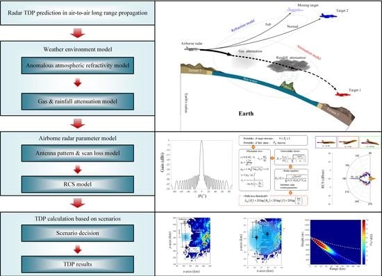
2. TDP Simulation Process

2.1. Anomalous Atmospheric Refractivity and Measurement

Figure 1 shows a conceptual figure of the air-to-air airborne radar wave propagation in accordance with an anomalous atmospheric environment. The gray and red aircrafts indicate an airborne radar and a target, which are located at heights of hr and ht, having a distance of Rt (slant range) and a horizontal range of Rh. The target is placed under various atmospheric conditions according to the wave refraction. To observe the wave refraction of the airborne radar, the refractive index needs be calculated using the measured atmospheric data such as temperature, air pressure, and relative humidity based on Equations (1)–(3), which are usually obtained by employing a rawinsonde or a GPS sonde [27,28,29].
N = ( n 1 ) 10 6 = 77.6 p T + e s 3.73 10 5 T 2
e s = r h 6.105 e x 100
x = 25.22 T 273.2 T 5.31 ln ( T 273.2 )
where p, T, rh indicate air pressure in hPa, temperature in K, and relative humidity in %. Then, the modified refractive index M at a height of h needs to be calculated using Equation (4) [30]. An example for a calculation of the modified refractive index M based on the measured data from Heuksando Meteorological Observatory [31] is listed in Table 1.
M = N + 0.157 h .
The gradient of the modified refractive index along the height ∇M can determine four common wave propagation refractions: normal refraction (79 < ∇M ≤ 157), super-refraction (0 < ∇M ≤ 79), sub-refraction (157 < ∇M), and ducting (∇M < 0). In accordance with these four refractions, the airborne radar wave propagation can become bent in the direction opposite or toward Earth’s surface, and it can be trapped in the ducting region. In particular, elevated ducts sometimes occur at high altitudes, which affect the wave propagation with a high path loss near the elevated ducting region. Thus, it is necessary to precisely model the refractivity of the elevated ducting in the air-to-air situation of the anomalous environment using a quad-linear model [32]. Figure 2a shows the conceptual figure of the quad-linear refractivity model. Four linear lines with slopes of m1, m2, m3, and m4 are used to model the refractivity, and the heights where the slope changes are h1, h2, and h3. Figure 2b represents the modified refractivity according to height using the quad-linear refractivity model in comparison with the actual refractivity data from a meteorological observatory. The measured refractivity data is interpolated using the typical linear interpolation method due to the sparse data along the height. The solid and dashed lines indicate the comparisons between the actual data from Heuksando Meteorological Observatory [31] on 25 July 2017 and the quad-linear model.
The dotted and dash-dotted lines denote those on September 26, 2017. To model the actual refractive index on July 25, 2017, the slopes of m1, m2, m3, and m4 are 125.9, 875, −25.6, and 142. The heights of h1, h2, and h3 are set to be 6223, 6239, and 6399 m. The second refractivity data on September 26, 2017, are also modeled using the quad-linear model (m1 = 140.8, m2 = −18.9, m3 = 142.6, m4 = 136.7, h1 = 5680 m, h2 = 5786 m, and h3 = 6459 m). These quad-linear refractivity models have 2001 data points along the altitude, which are employed as input parameters for the AREPS software to obtain the path loss according to the range and altitude. Furthermore, the other input parameters of the antenna beam pattern and DTED are also applied to the AREPS simulation to precisely estimate the air-to-air wave propagation path loss. The antenna beam pattern is derived by calculating the array factor of a 32 × 32 airborne radar array antenna using a triangular array configuration [31]. The array distances along the x- and y-axes are 0.475λ and 0.538λ at 10 GHz. This radiation pattern has a half-power beamwidth of 2.85° and a side lobe level of 13.5 dB. The DTED of the southwest region in South Korea are obtained from the Korean National Geographic Information Institute [33]. Then, the path loss computed using the AREPS software can be defined as LAREPS (m1, m2, m3, m4, h1, h2, h3, Rh, hr, ht) considering the anomalous environment. For example, with specific input parameters (m1 = m2 = m3 = m4 = 85, h1 = h2 = h3 = 15 km, Rh = 150 km, hr = 11 km, and ht = 5 km), we can obtain the path loss LAREPS of 163.5 dB in the elevated ducting of the anomalous atmospheric environment.

2.2. Weather Environment Models

Figure 3 illustrates the attenuation of the wave propagation by the atmospheric gases and rainfall. Such weather conditions can have a serious impact on the path loss, which is directly related to the TDP performance of the airborne radar. Hence, it is necessary to have the detailed attenuation models to increase the accuracy of the TDP estimation in the air-to-air airborne radar wave propagation. The atmospheric gas attenuation can be modeled based on ITU-R P.676-12 as follows [34]:
γ g = 0.1820 f ( N O x ( f ) + N W a t ( f ) )
N O x ( f ) = i S i , o x F i + N D ( f )
N W a t ( f ) = i S i , W a t F i
S i , o x = a 1 10 7 ( 300 T ) 3 exp [ a 2 ( 1 300 T ) ] P
S i , W a t = b 1 10 1 ( 300 T ) 3.5 exp [ b 2 ( 1 300 T ) ] e
L g = γ g R t
where γg is the specific gas attenuation in dB/km, and f is the frequency in GHz. NOx and NWat are the imaginary parts of complex refractivities in terms of oxygen and water vapor. Si,Ox and Si,Wat are the strengths of the ith oxygen and water vapor lines, and ND(f) is the dry continuum. P and e are dry air and water vapor partial pressures in hPa, and T is the absolute temperature in K. Fi is the oxygen or water vapor line shape. a1, a2, b1, and b2 are the line strength coefficients. The detailed coefficient values are listed in tables in [34]. Thus, the gas attenuation according to the range Rt can be defined as Lg in Equation (7).
In addition, the rainfall attenuation can be modeled based on ITU-R P.530-17, P.837-7, and P.838-3 as follows [35,36,37]:
γ r = κ ρ α
r = 1 0.477 R t 0.633 ρ 0.01 0.0173 α f 0.123 10.579 ( 1 exp [ 0.024 R t ] )
d e f f = r R t
L r = γ r d e f f
where γr is the specific rainfall attenuation in dB/km, and ρ is the rainfall precipitation in mm/h. α and κ are the rainfall attenuation parameters that depend on the frequency, polarization state, and angle of the signal path to the target. deff is the effective propagation distance considering the target range Rt multiplied by the scale factor of r. The rainfall attenuation in terms of the range can be defined as Lr in Equation (11).
In general, the precipitation is measured using rain gauge, weather radar, and satellite, and the measured weather information can be employed to calculate the rainfall attenuation [38,39,40,41,42,43]. To verify these attenuation models, we have investigated the attenuation measurements [41] and then some of the measurements according to the frequency with different precipitations are compared to the ITU-R attenuation models, as shown in Figure 4a. Furthermore, Figure 4b depicts the attenuation results compared with those of the measurement in accordance with the precipitation [42,43]. These comparison results demonstrate that the ITU-R model agrees well with the measurement, and this model can be adopted to increase the accuracy of the TDP in real atmospheric and weather environments. To predict the TDP along the range, we calculate atmospheric gas and rainfall attenuation results according to the range from 0 to 190 km, as presented in Figure 4c. The solid and dashed lines indicate the atmospheric gas attenuations in dry and wet weathers, and the water vapor densities for the dry and wet weathers are 0.1 and 18 g/m3 without the rainfall. The maximum attenuation values of the dry and wet weather conditions are 1.4 and 4.9 dB in the range from 0 to 190 km. The dotted and dash-dotted lines denote the rainfall attenuations in accordance with the precipitations of 10 mm/h and 30 mm/h, which are defined as the normal and heavy rain conditions in this research. The maximum attenuations in the normal and heavy rainfalls are 5.7 dB at 46.5 km and 15.1 dB at 54 km in the range from 0 to 190 km.
In the atmospheric environment modeling, it is important to consider uncertainties of the measurement for the atmospheric refractivity [44] and rainfall attenuation, which can possibly affect the TDP results. For example, if we make an assumption that the measurement of the refractivity had the uniform uncertainty of 2.5 % along the height, then the deviations between the original measurement and the uncertainties of the TDP can be increased up to 4.7% in the long-range over 80 km.

2.3. TDP Calculation with Airborne Radar Parameters

In Section 2.1, the refractive index, gas attenuation, rainfall attenuation, and radar parameters were modeled to estimate the total path loss of the wave propagation in an anomalous atmospheric environment; however, more radar parameters and computations are needed to accurately predict the TDP of the airborne radar. We determine the TDP using the threshold evaluations derived from the free-space path loss according to the range. To examine the threshold for the total path loss, the detectability factor is required for a given probability of detection and false alarm as written in Equation (14). In addition, the fluctuation loss is modeled using Equation (15) to calculate the TDP performance for describing the fluctuating target. Finally, these equations are directly related to the radar range equation for the detectable range that is introduced by Blake as follows [45]:
t = 0.9 ( 2 P d 1 ) ,    x 0 = ( g d + g f a ) 2
g d = ( 1.23 t 1 ( t ) 2 ) ,   g f a = 2.36 log 10 ( P f a ) 1.02
D ( P d ) = L f x 0 4 N p ( 1 + 1 + 16 N p x 0 )
L f ( P d ) = 1 ln ( P d ) ( 1 + g d g f a )
R f s ( P d ) = c 0 2 P t σ τ G 2 ( 4 π ) 3 k T [ D ( P d ) ] f 2 N f L s 4
where Pd is the detection probability ranging from 0 to 0.99, and Pfa indicates the false alarm rate of the airborne radar. Lf is the fluctuation loss in Swerling Case 1, and Np is the number of pulses integrated by the detector depending on the radar system. D is the detectability factor, and Rfs is the free-space detectable range in meters. c0 is the light speed of 3 × 10⁸ m/s, and σ is the RCS of the target in m2. k is the Boltzmann constant, and τ is the pulse length of the radar in seconds. Pt and G are transmitting power in watts and the array antenna gain, respectively. Nf and Ls are the noise figure and miscellaneous system loss of the radar. In the radar range Equation (16), it is required to set the system parameters of the airborne radar to specific values: Pt = 1 MW, τ = 2 μs, Pfa = 10−8, G = 103, k = 1.38 × 10⁻²³, f = 10 GHz, Nf = 100.5, and Ls = 100.3. Then, the total path loss of the threshold related to the TDP can be calculated by using the detectable range as follows:
L t o t ( P d ) = 20 log [ R f s ( P d ) ] + 20 log ( f ) + 20 log ( 4 π c 0 )
Figure 5 shows the calculated path loss threshold and detectability factor results according to the detection probability at a fixed RCS value of 8.5 m2. The path loss threshold varies from 151.4 to 159.2 dB when the Pd increases from 70% to 100%. The maximum detectability factor is 17.9. The total path loss threshold is significantly affected by the detectable range Rfs, and the detectability factor is dominantly decided by the fluctuation loss for the fluctuating type of the target. To further observe the TDP performance with the ranges and angles, we additionally compute the theoretical scan losses in terms of the scan angle ϕscan for the beam scanning of the radar array antenna, as written in Equation (18) [46,47].
L s c a n = cos n ( ϕ s c a n )
where Lscan is the scan loss of the radar, and n is the power of the cosine function set to be −2.5 in this research. Figure 6a presents the scan loss according to the scan angle. Due to the beam scanning, the array antenna gain can be gradually attenuated until 6.8 dB at the scanning angle of 70°. We also model a target aircraft using FEKO full EM software to obtain the RCSs at the azimuth angles. Figure 6b presents the RCS for the rear direction of the target aircraft. In the scanning angle, the maximum and averaged RCS values are 67.2 and 2.8 dBsm at the scan angles of 0° and 70°. With the environment models and the radar parameters, we can predict the total wave propagation loss for the airborne radar in the air-to-air situation. This total loss Ltot is then calculated to examine the TDP using Equation (19). For example, in the normal atmospheric environment, if the total path loss Ltot is 147.5 dB at Rt of 50 km, then the TDP can be obtained over 60% regardless of the target RCS. On the other hand, the TDP for very small targets with the RCS of lower than 2 m2 (typical military airborne) dramatically decrease for the long-range target over 100 km (Ltot > 154.2 dB).
L t o t = L A R E P S + L g + L r + L s c a n   [ d B ]

3. TDP Calculation with Airborne Radar Parameters

Figure 7 shows three air-to-air scenarios considered for the airborne radar TDP simulation in anomalous atmospheric environments. The detailed scenario explanations are as follows:
(1)
TDPs when azimuth beam scanning within 90° in an anomalous atmospheric environment of the refractivity, as shown in Figure 7a.
(2)
TDPs when azimuth beam scanning within 90° in a rainy weather environment, as shown in Figure 7b.
(3)
TDPs according to the distance (Rt < 190 km) to the target in a heavy rain environment, as shown in Figure 7c.
In all scenarios, the height hr of the airborne radar is consistent at 11 km, and the target height ht is set to be 5 km. Additionally, these scenarios are in the long-range radar propagation situations, which assumes that the slant range is almost same with the horizontal range (RtRh). The detailed explanations for the scenarios are listed in Table 2.
Figure 8a illustrates the simulation results of the TDP along the range and the azimuth angle for the first scenario, where the deep red and blue colors indicate the TDP of 100% and 0%. The TDP over 90% is obtained at the scan angle of 0° due to the high RCS level of the target aircraft, and the target is detected over the probability of 80% in the scan angle between −20° and 60° and the range from 50.5 to 153.8 km. On the other hand, the range from 0 to 50.2 km within the whole scan angle has the low TDP because this is the area below the airborne radar beam that cannot be reached. In addition, the scan loss of the airborne radar increases the path loss, which reduces the TDP in the wide angle from 60° to 90°. Figure 8b depicts the contour plot of the TDP over the 90% region according to the different atmospheric conditions of the refractivity. The solid, dashed, dotted, and dash-dotted lines denote the normal refraction, super-refraction, sub-refraction, and elevated ducting cases. We defined a detectable area by calculating the area inside the contour region to intuitively examine the TDP. The resulting detectable area of the super-refraction is larger than those of the others, which are similar to each other. It is because the super-refraction makes the wave propagation bend toward Earth’s surface, which results in low path loss levels over a large area. The summary of the detectable area results for TDPs over 80% and 90% is shown in Figure 8c.
Figure 9 illustrates the contour plot of the TDP over 80% according to the different weather conditions in the sub- and normal refractions for the second scenario. The solid and dashed lines indicate the TDP results according to the dry and rainy weather in the normal atmospheric condition, while the dotted and dash-dotted lines denote the results in the amorous atmospheric condition (super-refraction). In the dry weather, the TDP for the normal and super-refractions is similar to the results of the first scenario, where the detectable areas are 4738 and 6298 km2, respectively. In contrast, in rainy weather, the TDP of the airborne radar is extremely deteriorated because of the rainfall attenuation. The resulting detectable areas for the normal and super-refraction atmospheric environments are 1670 and 1734 km2. Note that the rainfall loss considerably affects the TDP of the airborne radar. In the third scenario, we additionally simulate and calculate the TDP of the airborne radar using another wave propagation simulation software (PETOOL) based on one-way and two-way split-step parabolic equation [48] and the ITU-R P.528-4 model [49] to confirm the results of the proposed process. Figure 10 shows the comparison of the TDP results along the target range of Rt using the different propagation models for the third scenario when the target and the airborne radar are gradually getting closer to each other. The airborne radar TDP becomes significantly low (almost zero TDP) when the heavy rainfall occurs. In the target range of Rt below 100 km, the AREPS simulation result well agrees with those of the PETOOL and ITU-R model. These results demonstrate that the proposed process is feasible for observing the TDP of the airborne radar considering the anomalous atmospheric environments.

4. Conclusions

In this paper, we proposed the TDP calculation process using the airborne long-range radar path loss based on the air-to-air scenarios in anomalous atmospheric and weather environments. The refractive index along an altitude was modeled using a quad-linear model. Then, the path loss including the refractivity model and other radar input parameters was simulated using the AREPS software along the range and the altitude. ITU-R models were used to consider the weather environment for the gas and rainfall attenuations according to the range. In addition, the radar beam scan loss and RCS of the target were considered to estimate the TDP of the airborne long-range radar. Various air-to-air scenarios were assumed for the airborne radar TDP simulation in the anomalous atmospheric and weather environments. In the first scenario, the target was detected over the probability of 80% in the scan angle between −20° and 60° and the range from 50.5 to 153.8 km. In the second scenario, the TDP of the airborne radar was extremely deteriorated in the rainfall weather because of the rainfall attenuation. The resulting detectable areas for the normal and super-refraction atmospheric environments were 1670 and 1734 km2. In the third scenario, the airborne radar TDP became significantly low due to the rainfall.

Author Contributions

Conceptualization, T.-H.L. and H.C.; methodology, T.-H.L. and H.C.; software, T.-H.L.; validation, T.-H.L. and H.C.; formal analysis, T.-H.L. and H.C.; investigation, T.-H.L. and H.C.; resources, T.-H.L. and H.C.; data curation, T.-H.L.; writing—original draft preparation, T.-H.L.; writing—review and editing, H.C.; visualization, T.-H.L. and H.C.; supervision, H.C.; project administration, H.C.; funding acquisition, H.C. All authors have read and agreed to the published version of the manuscript.

Funding

This research received no external funding.

Institutional Review Board Statement

Not applicable.

Informed Consent Statement

Informed consent was obtained from all subjects involved in the study.

Data Availability Statement

Not applicable.

Acknowledgments

This work was supported by a grant-in-aid of HANWHA SYSTEMS. This work was supported by the National Research Foundation of Korea (NRF) grant funded by the Korea government (MSIT) (NRF-2017R1A5A1015596). This research was supported by Basic Science Research Program through the National Research Foundation of Korea (NRF) funded by the Ministry of Education (No. 2015R1A6A1A03031833).

Conflicts of Interest

The authors declare no conflict of interest.

References

  1. Rim, J.-W.; Koh, I.-S. SAR image generation of ocean surface using time-divided velocity bunching model. J. Electromagn. Eng. Sci. 2019, 19, 82–88. [Google Scholar] [CrossRef]
  2. Farina, A.; Saverione, A.; Timmoneri, L. MVDR vectorial lattice applied to space–time processing for AEW radar with large instantaneous bandwidth. IEE Proc.-Radar Sonar Navig. 1996, 143, 41–46. [Google Scholar] [CrossRef]
  3. Kim, E.H.; Park, J. Dwell time optimization of alert-confirm detection for active phased array radars. J. Electromagn. Eng. Sci. 2019, 19, 107–114. [Google Scholar] [CrossRef]
  4. Nam, J.-H.; Rim, J.-W.; Lee, H.; Koh, I.-S.; Song, J.-H. Modeling of monopulse radar signals reflected from ground clutter in a time domain considering doppler effects. J. Electromagn. Eng. Sci. 2020, 20, 190–198. [Google Scholar] [CrossRef]
  5. Benzon, H.; Høeg, P. Wave propagation simulation of radio occultations based on ECMWF refractivity profiles. Radio Sci. 2015, 50, 778–788. [Google Scholar] [CrossRef]
  6. Barclay, M.; Pietzschmann, U.; Gonzalez, G.; Tellini, P. AESA upgrade option for Eurofighter captor radar. IEEE Aerosp. Electron. Syst. Mag. 2010, 25, 11447006. [Google Scholar] [CrossRef]
  7. Mesnard, F.; Sauvageot, H. Climatology of anomalous propagation radar echoes in a coastal area. J. Appl. Meteorol. Climatol. 2010, 49, 2285–2300. [Google Scholar] [CrossRef]
  8. Lenouo, A. Climatology of anomalous propagation radar over Douala, Cameroon. Meteorol. Appl. 2014, 21, 249–255. [Google Scholar] [CrossRef]
  9. Colussi, L.C.; Schiphorst, R.; Teinsma, H.W.M.; Witvliet, B.A.; Fleurke, S.R.; Bentum, M.J.; van Maanen, E.; Griffioen, J. Multiyear trans-horizon radio propagation measurements at 3.5 ghz. IEEE Trans. Antennas Propag. 2018, 66, 884–896. [Google Scholar] [CrossRef]
  10. López, R.N.; del Río, V.S. High temporal resolution refractivity retrieval from radar phase measurements. Remote Sens. 2018, 10, 896. [Google Scholar] [CrossRef] [Green Version]
  11. Wang, L.; Wei, M.; Yang, T.; Liu, P. Effects of atmospheric refraction on an airborne weather radar detection and correction method. Adv. Meteorol. 2015, 2015, 407867. [Google Scholar] [CrossRef]
  12. Gerstoft, P.; Rogers, L.T.; Krolik, J.L.; Hodgkiss, W.S. Inversion for refractivity parameters from radar sea clutter. Radio Sci. 2003, 38, 8053. [Google Scholar] [CrossRef]
  13. Lowry, A.R.; Rocken, C.; Sokolovskiy, S.V.; Anderson, K.D. Vertical profiling of atmospheric refractivity from ground-based GPS. Radio Sci. 2002, 37, 1–19. [Google Scholar] [CrossRef]
  14. Liu, X.; Wu, Z.; Wang, H. Inversion method of regional range-dependent surface ducts with a base layer by doppler weather radar echoes based on WRF model. Atmosphere 2020, 11, 754. [Google Scholar] [CrossRef]
  15. Wagner, M.; Gerstoft, P.; Rogers, T. Estimating refractivity from propagation loss in turbulent media. Radio Sci. 2016, 51, 1876–1894. [Google Scholar] [CrossRef] [Green Version]
  16. Gunashekar, S.D.; Warrington, E.M.; Siddle, D.R.; Valtr, P. Signal strength variations at 2 GHz for three sea paths in the British Channel Islands: Detailed discussion and propagation modeling. Radio Sci. 2007, 42, 1–13. [Google Scholar] [CrossRef] [Green Version]
  17. Wang, Q.; Alappattu, D.P.; Billingsley, S.; Blomquist, B.; Burkholder, R.J.; Christman, A.J.; Creegan, E.D.; Paolo, T.; de Eleuterio, D.P.; Fernando, H.J.S.; et al. CASPER: Coupled air–sea processes and electromagnetic ducting research. Bull. Am. Meteorol. Soc. 2018, 99, 1449–1471. [Google Scholar] [CrossRef]
  18. Habib, A.; Moh, S. Wireless channel models for over-the-sea communication: A comparative study. Appl. Sci. 2019, 9, 443. [Google Scholar] [CrossRef] [Green Version]
  19. Shi, Y.; Kun-De, Y.; Yang, Y.-X.; Ma, Y.-L. Influence of obstacle on electromagnetic wave propagation in evaporation duct with experiment verification. Chin. Phys. B 2015, 24, 054101. [Google Scholar] [CrossRef]
  20. Wang, S.; Lim, T.H.; Chong, Y.J.; Ko, J.; Park, Y.B.; Choo, H. Estimation of abnormal wave propagation by a novel duct map based on the average normalized path loss. Microw. Opt. Technol. Lett. 2020, 62, 1662–1670. [Google Scholar] [CrossRef]
  21. Barrios, A.E. Considerations in the development of the advanced propagation model (APM) for U.S. Navy applications. In Proceedings of the 2003 International Conference on Radar, Adelaide, SA, Australia, 3–5 September 2003; pp. 77–82. [Google Scholar]
  22. Sirkova, I. Brief review on PE method application to propagation channel modeling in sea environment. Open Eng. 2012, 2, 19–38. [Google Scholar] [CrossRef]
  23. Levy, M. Parabolic Equation Methods for Electromagnetic Wave Propagation; The Institution of Engineering and Technology: London, UK, 2000. [Google Scholar]
  24. Hardin, R.H.; Tappert, F.D. Application of the split-step Fourier method to the numerical solution of nonlinear and variable coefficient wave equations. SIAM Rev. 1973, 15, 423. [Google Scholar]
  25. Ozgun, O. New Software Tool (GO+UTD) for visualization of wave propagation [testing ourselves]. IEEE Antennas Propag. Mag. 2016, 58, 91–103. [Google Scholar] [CrossRef]
  26. Patterson, W.L. User Manual for Advanced Refractive Effects Prediction System (AREPS); Space Naval Warfare System Center: San Diego, CA, USA, 2004. [Google Scholar]
  27. Schwartz, B.; Benjamin, S.G. A comparison of temperature and wind measurements from ACARS-equipped aircraft and Rawinsondes. Weather Forecast. 1995, 10, 528–544. [Google Scholar] [CrossRef]
  28. Lee, T.R.; Pal, S. On the potential of 25 years (1991–2015) of rawinsonde measurements for elucidating climatological and spatiotemporal patterns of afternoon boundary layer depths over the contiguous US. Adv. Meteorol. 2017, 2017, 6841239. [Google Scholar] [CrossRef] [Green Version]
  29. Hock, T.F.; Franklin, J.L. The NCAR GPS dropwindsonde. Bull. Amer. Meteorol. Soc. 1999, 80, 407–420. [Google Scholar] [CrossRef] [Green Version]
  30. ITU. The Radio Refractive Index: Its Formula and Refractivity Data. Available online: https://www.itu.int/rec/R-REC-P.453/en (accessed on 24 August 2021).
  31. Korea Meteorological Administration. Available online: https://www.kma.go.kr/eng/index.jsp (accessed on 24 August 2021).
  32. Lim, T.H.; Go, M.; Seo, C.; Choo, H. Analysis of the target detection performance of air-to-air airborne radar using long-range propagation simulation in abnormal atmospheric conditions. Appl. Sci. 2020, 10, 6440. [Google Scholar] [CrossRef]
  33. National Geographic Information Institute. Available online: https://www.ngii.go.kr/eng/main.do? (accessed on 24 August 2021).
  34. ITU. Attenuation by Atmospheric Gases and Related Effects. Available online: https://www.itu.int/rec/R-REC-P.676-12-201908-I/en (accessed on 24 August 2021).
  35. ITU. Propagation Data and Prediction Methods Required for the Design of Terrestrial Line-of-Sight Systems. 2017. Available online: https://www.itu.int/rec/R-REC-P.530-17-201712-I (accessed on 24 August 2021).
  36. ITU. Characteristics of Precipitation for Propagation Modelling, International Telecommunication Union 2017. Available online: https://www.itu.int/rec/R-REC-P.837-7-201706-I/en (accessed on 24 August 2021).
  37. ITU. Specific Attenuation Model for Rain for Use in Prediction Methods 2005. Available online: https://www.itu.int/rec/R-REC-P.838-3-200503-I/en (accessed on 24 August 2021).
  38. Shayea, I.; Rahman, T.A.; Azmi, M.H.; Islam, R. Real measurement study for rain rate and rain attenuation conducted over 26 Ghz microwave 5G link system in Malaysia. IEEE Access 2018, 6, 19044–19064. [Google Scholar] [CrossRef]
  39. Nalinggam, R.; Ismail, W.; Singh, M.J.; Islam, M.T.; Menon, P.S. Development of rain attenuation model for Southeast Asia equatorial climate. IET Commun. 2013, 7, 1008–1014. [Google Scholar] [CrossRef]
  40. Shrestha, S.; Choi, D.-Y. Rain attenuation study over an 18 GHz terrestrial microwave link in South Korea. Int. J. Antennas Propag. 2019, 2019, 1712791. [Google Scholar] [CrossRef] [Green Version]
  41. Shebani, N.M.; Kaeib, A.F.; Zerek, A.R. Estimation of rain attenuation based on ITU-R model for terrestrial link in Libya. In Proceedings of the 5th International Conference of Control Signal Processing, Kairouan, Tunisia, 28–30 October 2017. [Google Scholar]
  42. Kestwal, M.C.; Joshi, S.; Garia, L.S. Prediction of rain attenuation and impact of rain in wave propagation at microwave frequency for tropical region (Uttarakhand, India). Int. J. Microw. Sci. Technol. 2014, 2014, 958498. [Google Scholar] [CrossRef] [Green Version]
  43. Islam, R.; Rahman, T.A.; Karfaa, Y. Worst-month rain attenuation statistics for radio wave propagation study in Malaysia. In Proceedings of the 9th Asia-Pacific Conference on Communications, Penang, Malaysia, 21–24 September 2003; Volume 3, pp. 1066–1069. [Google Scholar]
  44. Jicha, O.; Pechac, P.; Kvicera, V.; Grabner, M. On the uncertainty of refractivity height profile measurements. IEEE Antennas Wirel. Propag. Lett. 2011, 10, 983–986. [Google Scholar] [CrossRef]
  45. Blake, L.V. Radar Range-Performance Analysis; Munro Pub. Co.: Silver Spring, MD, USA, 1991. [Google Scholar]
  46. Mailloux, R.J. Phased Array Antenna Handbook, 3rd ed.; Artech House: Norwood, MA, USA, 2018. [Google Scholar]
  47. Nathanson, F.E.; O’Reilly, P.J.; Cohen, M.N. Radar Design Principles: Signal Processing and the Environment; Scitech Publ.: Raleigh, NC, USA, 2004. [Google Scholar]
  48. Ozgun, O.; Apaydin, G.; Kuzuoglu, M.; Sevgi, L. PETOOL: MATLAB-based one-way and two-way split-step parabolic equation tool for radiowave propagation over variable terrain. Comput. Phys. Commun. 2011, 182, 2638–2654. [Google Scholar] [CrossRef]
  49. ITU. A Propagation Prediction Method for Aeronautical Mobile and Radionavigation Services Using the VHF, UHF and SHF Bands 2019. Available online: https://www.itu.int/rec/R-REC-P.528-4-201908-I/en (accessed on 24 August 2021).
Figure 1. Airborne radar wave propagation for TDP in accordance with anomalous atmospheric environment.
Remotesensing 13 03943 g001
Figure 2. Modified refractivity according to height: (a) the quad-linear refractivity model; (b) comparisons between the actual refractivity data and the quad-linear models.
Remotesensing 13 03943 g002
Figure 3. Wave propagation attenuation by atmospheric gases and rainfall.
Remotesensing 13 03943 g003
Figure 4. Calculated atmospheric gas and rainfall attenuation results: (a) rainfall attenuation according to frequency; (b) rainfall attenuation according to precipitation; (c) gas and rainfall attenuation according to range.
Remotesensing 13 03943 g004
Figure 5. Calculated path loss threshold and detectability factor results according to detection probability.
Remotesensing 13 03943 g005
Figure 6. Scan loss and target RCS according to scan angle: (a) scan loss according to scan angle; (b) RCS of a target aircraft.
Remotesensing 13 03943 g006
Figure 7. Three air-to-air scenarios for the TDP simulation in anomalous atmospheric environments: (a) azimuth beam scanning in an anomalous atmospheric environment; (b) azimuth beam scanning in a rainy environment; (c) encountering a target in a heavy rain environment.
Remotesensing 13 03943 g007
Figure 8. Simulation results of the TDP along the range and the azimuth angle for the first scenario: (a) TDP in a super-refraction; (b) contour plots of TDP in an anomalous atmospheric environment; (c) detectable area results for TDPs over 80% and 90%.
Remotesensing 13 03943 g008aRemotesensing 13 03943 g008b
Figure 9. Contour plot of TDP according to different weather conditions in the sub- and normal refractions for the second scenario.
Remotesensing 13 03943 g009
Figure 10. Comparison of TDP along the range using different propagation models for the third scenario.
Remotesensing 13 03943 g010
Table 1. Modified refractive index based on measured data (3 January 2017).
Height (m)Air Pressure (hPa)Temperature (°C)Relative Humidity (%)Refractivity (M-Unit)
801015687333.7
752.2934.84.59.6383.3
1477.2855.14.714.5476.7
2229.8779.62.910.1572.9
2999.6708.2–2.710.6676.9
3793.1640.3–7.910.3784.7
Table 2. TDP simulation scenarios.
Scenario IScenario IIScenario III
Scan range (Rt)0–190 km0–190 km0–190 km
Elevation steering angle−4.3°−4.3°−1.8–31°
Scan angle (ϕscan)−20–70°−20–70°
Atmospheric condition (∇M)Normal (∇M = 85)
Sub (∇M = 300)
Super (∇M = 10)
Ducting (∇M = −80)
Normal (∇M = 85)
Super (∇M = 10)
Normal (∇M = 85)
Weather condition (e)Dry (0.1 g/m3)Dry (0.1 g/m3)
Rainfall
(12 mm/h)
Dry (0.1 g/m3)
Heavy rainfall
(22 mm/h)
Publisher’s Note: MDPI stays neutral with regard to jurisdictional claims in published maps and institutional affiliations.

