Retrieval of Water Quality from UAV-Borne Hyperspectral Imagery: A Comparative Study of Machine Learning Algorithms

Abstract

The rapidly increasing world population and human activities accelerate the crisis of the limited freshwater resources. Water quality must be monitored for the sustainability of freshwater resources. Unmanned aerial vehicle (UAV)-borne hyperspectral data can capture fine features of water bodies, which have been widely used for monitoring water quality. In this study, nine machine learning algorithms are systematically evaluated for the inversion of water quality parameters including chlorophyll-a (Chl-a) and suspended solids (SS) with UAV-borne hyperspectral data. In comparing the experimental results of the machine learning model on the water quality parameters, we can observe that the prediction performance of the Catboost regression (CBR) model is the best. However, the prediction performances of the Multi-layer Perceptron regression (MLPR) and Elastic net (EN) models are very unsatisfactory, indicating that the MLPR and EN models are not suitable for the inversion of water quality parameters. In addition, the water quality distribution map is generated, which can be used to identify polluted areas of water bodies.

1. Introduction

Inland water is the most significant freshwater resource for humans. It has various functions, including water storage, irrigation, and power generation. Inland water bodies are usually close to human settlements. They are easily subject to the combined pressures caused by intensive human activities and environmental changes. Pollution, such as agricultural activities, aquaculture, and industrial discharge, will lead to the accumulation of nutrients in the water and will cause eutrophication [1]. The eutrophication will further lead to the occurrence of algal blooms [2]. These destroy the aquatic ecological structure and consume a large amount of dissolved oxygen, leading to hypoxia and cause the death of aquatic animals and plants. Therefore, for the sustainable development of water resources, water quality must be monitored by statutes on a chemical, physical, and biological basis, according to the Environmental Quality Standards for Surface Water (GB3838-2000) in China [3]. Water quality parameters are the most commonly used evaluation measurements to characterize the water quality of inland water bodies.

Chlorophyll-a (Chl-a) concentration and Suspended solids (SS) concentration are the most common water quality parameters. Chl-a is a typical optical active parameter widely existing in algae and cyanobacteria, as well as in other aquatic plants. The concentration of Chl-a is an indicator for the eutrophication of water bodies based on nutrient availability, quantifying the nutritional status of water bodies [4]. High concentrations of SS will reduce the light transmittance of the water and increase the water-leaving reflectance in the visible wavelength. The concentration of SS in water is also directly related to the migration of pollutants such as heavy metals and organics [5]. Therefore, it is essential to monitor the concentration of SS in the aquatic system.

The conventional methods for water quality monitoring are mainly based on field sampling and laboratory analysis, which are expensive, time-consuming, and labor-intensive [6]. With the development of remote sensing technology, remote sensing has been used as a supplement for traditional methods in aquatic ecosystem monitoring because of its convenient acquisition, long-term dynamic monitoring, and inexpensive qualities. Huang et al. evaluated the spatial variation of Chl-a using MODIS data for different river flow conditions [7]. Doña et al. predicted and assessed the dynamics the diversification of Chl-a and transparency using MODIS, TM, and ETM+ data [8]. Du et al. investigated the tempo-spatial dynamics pattern of water quality in the Taihu Lake estuary using GOCI imagery [9]. Syariz et al. used spectral and spatial information from Sentinel-3 images to retrieval the concentration of Chl-a [10]. Rajesh et al. predicted the heavy metal concentration in water including Arsenic (As), cadmium (Cd), chromium (Cr), copper (Cu), iron (Fe), lead (Pb), nickel (Ni), zinc (Zn), aluminum (Al), cobalt (Co), manganese (Mg), beryllium (Be), boron (B), lithium (Li), molybdenum (Mo), selenium (Se), and vanadium (V), using Cartosat-2 data and measuring data [11]. Rostom et al. predicted and assessed the concentration of heavy metals including Cr, Mn, Fe, Co, Ni, Cu, Zn, Cd, and Pb in water using hyperspectral remote sensing data [12]. The studies mentioned above have researched the application of satellite remote sensing data for water quality monitoring. However, it is challenging to assess water quality in inland water bodies with the coarse spatial resolution and spectral resolution of satellite data. UAV-borne remote sensing hyperspectral data with high spatial resolution, spectral resolution, and timeliness is superior to satellite data. Therefore, the water quality parameters’ concentration can be predicted and retrieved using UAV-borne hyperspectral data.

The spectral reflectance information extracted from remote sensing imagery can be used to estimate the concentrations of water quality parameters. Meanwhile, artificial intelligence technology is widely used in the water quality monitoring field in recent years. Quan et al. used a genetic algorithm (GA) to optimize the parameters of the support vector machine regression (SVR) model for the prediction of vertical water temperature and water temperature structure [13]. Leong et al. used the support vector machine (SVM) and least-squares support vector machine (LS-SVM) to predict water quality parameters including dissolved oxygen (DO), biological oxygen demand (BOD), chemical oxygen demand (COD), suspended solids (SS), pH value (PH), and ammoniacal nitrogen (AN) [14]. Lu et al. used the extreme gradient boosting (XGBoost) model and random forest (RF) model to predict water quality parameters including temperature, DO, specific conductance, pH value, turbidity, and fluorescent dissolved organic matter [15]. Najah Ahmed et al. proposed a neuro-fuzzy inference system (ANFIS)-based augmented wavelet de-noising technique (WDT) to predict water quality parameters including AN, SS, and pH [16]. Sharafati et al. used adaboost regression (ABR), gradient boost regression (GBR), and random forest regression (RF) to predict water quality parameters including total dissolved solids (TDS), five-day biochemical oxygen demand (BOD₅), and COD on a daily scale [17]. Parsimehr et al. used the multilayer perceptron artificial neural network to predict and simulate the COD of the Gamasiab river [18]. Xiaojuan et al. used ensemble learning models based on four models, including the k-nearest neighbors (KNN), artificial neural network (ANN), SVR, and RF, to retrieve Chl-a and TN in water [19]. Although researchers have conducted numerous studies, there is still a lack of analyses on different machine learning algorithms using UAV-borne hyperspectral data.

The machine learning model can quickly acquire the required information from the data but different models have different characteristics. Therefore, the main aims of this study are (1) to compare and analyze the prediction performance of different machine learning models, including CBR, Adaboost regression (ABR), extreme boost regression (XGBR), random forest (RF), extremely randomized trees (ERT), support vector regression (SVR), MLPR, and EN, using the evaluation index including R², RMSE, and MAE; (2) to use typical water quality parameters, including Chl-a and SS, to evaluate the machine learning model; and (3) to verify the potential of machine learning models combined with UAV-borne hyperspectral data in water quality mapping.

2. Materials and Methods

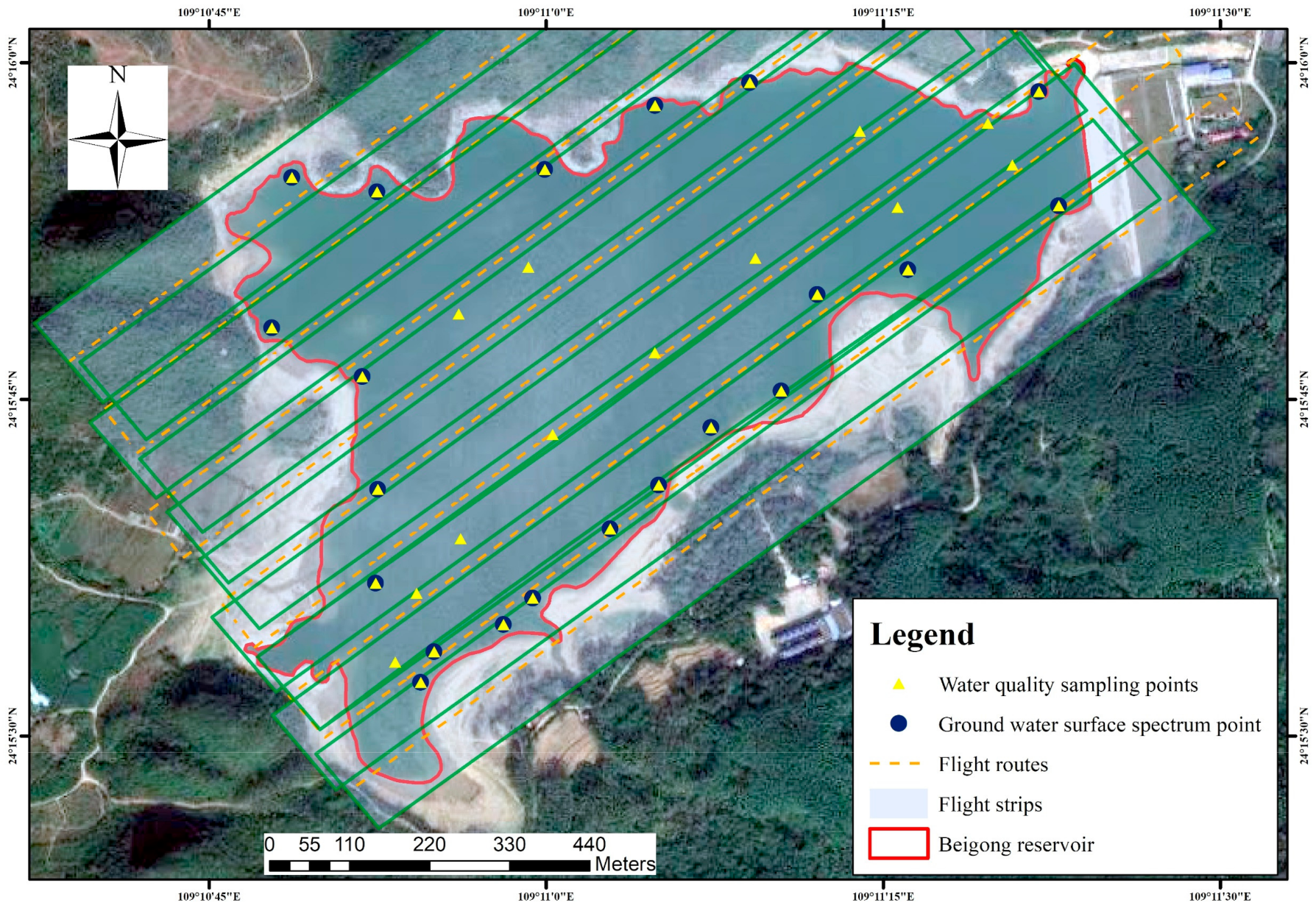
2.1. Study Area

The study area was Beigong Reservoir (114°21′14.15″ E, 30°35′5.52″ N) with a catchment area of 6.8 ${\mathrm{km}}^2$ and a storage capacity of 12.2 × 10⁶ m³, which is the primary supply source for the tributary of the Liu River, namely the Pearl River basin of the Xijiang river system. Beigong Reservoir is located in the Beigong village southwest of Liuzhou, Guangxi Zhuang Autonomous Region, China. Additionally, Liuzhou is an essential industrial city in Guangxi and is key to the “three wastes” emissions of exhaust gas, wastewater, and waste residue. Moreover, the Liuzhou Municipal Government attaches great importance to the local water pollution problem. Beigong Reservoir is a medium-sized reservoir, utilized for irrigation, flood control, and power generation. It is a famous tourist attraction with a beautiful scenery surrounded by mountains that integrates entertainment, tourism, and life functions. Hence, the Beigong Reservoir is of great significance for the residents and policymakers.

2.2. Data Collection

Liuzhou’s summers are long, hot, sultry, humid, and cloudy, and the winters are short, cold, and mostly sunny. During the year, the temperature usually varies between 6 °C and 33 °C, and is rarely below 2 °C or above 36 °C. Therefore, the best time to conduct a water quality sampling survey is from the last ten-day period of September to October. Therefore, field investigations were uniformly conducted in Beigong Reservoir from 9 to 10 September 2018. On the basis of the field data collection regulations, 33 sample points at Beigong Reservoir were collected for Chl-a and SS inversion. The field sampling data were analyzed in the laboratory. The statistical information of the water sampling data is shown in

Table 1. Statistical information of the water sampling data in Beigong Reservoir including Chl-a (mg/m³) and SS (mg/L).

Water Quality Parameters	Range	Average Value	Standard Deviation
Chl-a (n = 33)	3.54~14.2 (mg/m3)	8.03	2.32
SS (n = 33)	2~18 (mg/L)	5.86	4.54

. Detailed information about the Beigong Reservoir is presented in Figure 1, in which the water quality sampling points, ground water surface spectrum point, the UAV-flight routes, and the obtained UAV-borne flight strips are shown.

The ground water surface spectral reflectance data will be discussed next. The ground water surface spectrum was collected by the ASD FieldSpec 3 field-portable spectrometer with a wavelength range of 350–2500 nm. The spectrometer was provided by the China University of Geosciences (Wuhan, China). The measurement of the ground water surface spectrum was based on the “above-water surface method” [20]. The reference board with a reflectivity of nearly 1 was used for radiometric calibration. In windless weather, the water surface was flat. The water surface spectrum, sky spectrum, and synchronously the spectral data of the reference board were collected. The reference board was utilized to perform the calibration of the water surface spectrum and to obtain the water-leaving reflectance data. The ground water surface spectral reflectance collection was repeated three times in situ and the average value of the three collected data was used as the final reflectance data. The total radiance received by the spectrometer can be expressed as:

$$L\_sw=L_w+r{L}_{sky}$$

(1)

where $L\_sw$ is the total radiance received by the spectrometer. $L_w$ is the water-leaving radiance. $L_{sky}$ is the diffuse radiance of the sky. r is the air–water interface reflectance rate. When the water surface is flat, r can be set as 0.022; when the wind speed is about 5 m/s, r can be set as 0.025; and when the wind speed is about 10 m/s, r can be set as 0.026–0.028. $L_w$ can be expressed as follows [21]:

$$R_{rs}=\frac{L_w}{E_d(0^{+})}=\frac{(L_{\_sw}-r{L}_{sky})}{\pi L_p}{\rho }_p$$

(2)

$$E_d(0^{+})={\mathrm{L}}_p\frac{\pi }{{\rho }_p}$$

(3)

where $E_d(0^{+})$ is the incident total irradiance. ${\mathrm{L}}_p$ is the 100% converted value of the reference board. $R_{rs}$ is the water-leaving reflectance.

The UAV-borne hyperspectral data will be discussed next. We adopted the six-rotor DJ M600 Pro UAV as the airborne platform and the sensor installed on it was the Headwall NANO-Hyperspec manufactured by Headwall Photonics Lnc. The spectral resolution was 6.0 nm [22,23]. The resampling interval was set to 2.2 nm, which is the sensor parameter. At the UAV flight process, the field of view was 16° and the flying height of the UAV was 400 m with a real-time wind speed of 5.2 m/s. According to the area of the reservoir, 10 routes of flight have been designed, where the along-track overlap was 80% and the side overlap was 60% [24]. With 270 spectral bands in the range of 400–1000 nm, the spatial resolution of the hyperspectral imagery was 0.173 m/pixel. Due to the low flight altitude, atmospheric influence can be ignored [25]. The UAV-borne hyperspectral image preprocessing was conducted, including water body extraction, sensor calibration, geometric correction, and in situ radiation correction. Firstly, the normalized difference water index (NDWI) was used to extract the water information in the UAV-borne image [26,27,28]. Secondly, we performed geometric correction for the image. The NANO-Hyperspec hyperspectral imaging spectrometer has a global positioning system and an inertial measurement unit (GPS/IMU) navigation system that can contribute to geometrically correcting the image by recording the position and attitude information of the spectrometer. Thirdly, regarding the calibration of the sensors, the signal output by the sensor unit was converted into the actual radiation intensity value. Finally, by constructing the linear relationship between the pixel spectrum of the UAV hyperspectral image and the ground water spectrum, the in situ radiation calibration was performed [29]. The water quality sampling data, the ground water surface spectral reflectance data, and UAV-borne hyperspectral data were all collected at the same time.

2.3. Method

2.3.1. Machine Learning Algorithms Used for the Estimation of Water Quality Parameters

Adaboost Regression (ABR)

ABR is a typical boosting algorithm introduced by Freund [30]. ABR trains the weak learners and then integrates the trained weak learners to obtain a final model [31]. ABR assigns different weights to each sample according to the prediction error rate of the learner, then adjusts the weight of the sample, and finally accumulates and weights the prediction results of all learners to generate a predicted value.

Gradient Boost Regression tree (GBRT)

GBRT is a machine learning algorithm based on ensemble decision trees [32], which is the regression form of gradient boost decision trees (GBDT). The GBRT model first builds a regression tree with equal weights based on the original data. It evaluates the prediction results by minimizing the square error. The smaller the mean square error, the lower the weight of the decision tree. The GBRT model uses the negative gradient of the loss function in the current model to approximate the residual between the current model’s predicted value and the observed value, so that the model optimizes the weight of the regression tree along the direction of the negative gradient of the loss function. In each round of the training process, the model reduces the loss function and accelerates the convergence to reach the local optimal solution or the global optimal solution. Through continuous iteration, the predicted values of all the regression trees are combined to obtain the final prediction result.

Extreme Gradient Boosting Regression (XGBR)

XGBR is an improved decision tree algorithm based on the GBDT algorithm [33]. The core of the algorithm is to continuously add and train new decision trees to fit the residuals of the previous iteration [34] and the prediction values of all the decision trees are accumulated to obtain the final prediction result. XGBR improves prediction performance by reducing model bias. Compared with the traditional GBDT algorithm, XGBR modifies the objective function of the GBDT algorithm. The formula of the loss function is defined as follows:

$${\mathrm{Loss}}^{(\mathrm{t})}={\displaystyle \sum _{i=1}^T[g_i{f}_t(x_i)+\frac{1}{2}{h}_i{f}_t^2(x_i)]}+\Omega (f_t)$$

(4)

$$g_i={\partial }_{{\widehat{y}}^{(t-1)}}l(y_{i,}{\widehat{y}}_i^{{}^{(t-1)}}),h_i={\partial }_{{\widehat{y}}^{(t-1)}}^{2}l(y_{i,}{\widehat{y}}_i^{{}^{(t-1)}})$$

(5)

$$\Omega (f_{\mathrm{t}})=\gamma T+\frac{1}{2}\lambda {\displaystyle \sum _{n=1}^T{w}_n^2}$$

(6)

where $g_i$ and $h_i$ are the first and second partial derivatives of the loss function. ${\widehat{y}}_i$ is the predicted value of the model, while $y_i$ is the observed value. $f_{\mathrm{t}}(x_i)$ represents the score of the i-th sample in the t-th decision tree, $\Omega (f_{\mathrm{t}})$ is the regular term of the model, $l$ represents the number of trees, $\gamma$ represents the complexity of the leaves, T represents the number of the leaves,$\lambda$ represents the scaler factor, and $w_n$ represents the weight of the n-th leaf node in the tree.

After removing the constant term, the final objective function can be expressed as:

$$\mathrm{Loss}=-\frac{1}{2}{\displaystyle \sum _{j=1}^T\frac{G_n^2}{H_n+\lambda }+\gamma T}$$

(7)

where $\frac{G_n^2}{H_n+\lambda }$ represents the contribution of each leaf node to the current model loss function. XGBR uses a greedy algorithm to traverse all split leaf nodes in the model. When the gain of the target after the split is less than the set threshold, we can ignore the split.

$$\begin{array}{l}\mathrm{Gain}=\frac{1}{2}[\frac{G_L^2}{H_L+\lambda }+\frac{G_R^2}{H_R+\lambda }-\frac{{(G_L+G_R)}^2}{H_L+H_R+\lambda }]-\gamma >0\\ \end{array}$$

(8)

where $\frac{G_L^2}{H_L+\lambda }$ represents the left subtree score, $\frac{G_R^2}{H_R+\lambda }$ represents the right subtree score, and $\frac{{(G_L+G_R)}^2}{H_L+H_R+\lambda }$ represents the score when it is not divided.

Catboost Regression (CBR)

CBR is a new decision tree based on a gradient boosting frame [35] and uses oblivious decision trees as a based learner. Oblivious trees use the same criteria for splitting at each level of the tree. Each leaf index can be encoded as a binary vector whose length is equal to the depth of the tree, which helps to avoid overfitting and speed up the prediction of the model. CBR differs from the traditional GBDT algorithm in three aspects: (1) CBR can efficiently process categorical features. The categorical feature refers to a category or label. Unlike other numerical characteristics, the numerical variables of categorical characteristics cannot be compared with other numerical variables. Therefore, they are also called non-ordered features. Discrete numbers are also categorical features. In the traditional GBDT algorithm, when the structure and distribution of the training data set and the test data set are different, the conditional offset problem will appear. Furthermore, CBR uses the improved greedy target statistics method to add prior distribution items to reduce the influence of noise and low-frequency data on the data distribution. For regression, prior items can take the mean of the data set label. (2) When CBR constructs a new split node for the current tree, it uses a greedy method to consider all combinations which combine different types of features into new features and dynamically transform the new composite categorical features into numeric features. (3) CBR replaces the gradient estimation method in the traditional algorithm by ordered boosting, which helps to overcome the prediction shift caused by gradient bias.

Random Forest (RF)

RF uses the bootstrap method to randomly select n samples from the original data to construct a decision tree. Each sample has M attributes. In the node split of the decision tree, m attributes are randomly selected from the M attributes using the information gain method, where in the attribute with the largest gain is selected as the best split attribute of the node. Then, the prediction results of multiple decision trees are averaged to obtain the final prediction result [36].

Extremely Randomized Trees (ERT)

The structure of the ERT [37] is similar to the RF. The difference between the ERT and RF is that the ERT uses all the samples to construct a decision tree in the training process. For node splitting, the RF algorithm selects the best attribute split, while the ERT randomly selects the attribute split [38], which results in the size of the generated decision tree being larger than that generated by the RF model. Therefore, the variance of the ERT model is reduced compared to the RF model.

Support Vector Machine (SVM)

SVR is a kernel-based algorithm that improves the model’s generalization ability by seeking the minimum structured risk and realizing the experience risk minimization. SVR can obtain good prediction results with a small sample size [39].

Multi-Layer Perceptron Regression (MLPR)

MLPR is the most commonly used artificial neural network model, which is composed of three types of layers: an input layer, an output layer, and one or more hidden layers with activation functions [40]. It uses a subset of the training set to adjust the weight and biases on each node of layers. MLPR takes input data, multiplies them with weights, and then inputs them into the activation function to produce final results. MLPR can obtain non-linear relationships and real-time learning. However, MLPR requires many hyperparameters to be adjusted, which is time-consuming.

Elastic Net (EN)

EN is a mixture of the Lasso regression (LR) and the Ridge regression (RR) [41], and the optimization objective function of elastic net regression is defined as follows:

$$\underset{\beta \in R^p}{\arg \min }\{\parallel y-X\beta {\parallel }^2+ \lambda [(1-\alpha )\parallel \beta {\parallel }_2+ \alpha \parallel \beta {\parallel }_1]\}$$

(9)

where $\parallel \cdot {\parallel }_2$ represents the L2 norm and $\parallel \cdot {\parallel }_1$ represents the L1 norm. The EN regression penalty function uses the convex combination of the L1 norm and L2 norm, which is equally the convex combination of the RR penalty function and LR penalty function. Therefore, the EN has the advantages of both RR and LR, which not only achieves the purpose of variable selection but also improves the stability of the model. It automatically selects variables and retains important features, as well as eliminates irrelevant features.

2.3.2. Model Evaluation

In this study, we evaluate the models’ performance via three indicators, including the coefficient of determination (R²), root mean square errors (RMSE) and mean absolute error (MAE). These indicator metrics can be calculated as follows:

$${\mathrm{R}}^2(y,\widehat{y})=1-\frac{{\displaystyle {\sum }_{i=1}^N{(y_i-{\widehat{y}}_i)}^2}}{{\displaystyle {\sum }_{i=1}^N{(y_i-{\overline{y}}_i)}^2}}$$

(10)

$$\mathrm{RMSE}(y,\widehat{y})=\sqrt{\frac{{\displaystyle {\sum }_{i=1}^N{(y_i-{\widehat{y}}_i)}^2}}{N}}$$

(11)

$$\mathrm{MAE}(y,\widehat{y})=\frac{1}{N}{\displaystyle \sum _{i=1}^N|{\widehat{y}}_i-y_i|}$$

(12)

where $y_i$ is the observed value, ${\overline{y}}_i$ is the average of the observed value, and N is the number of valid samples used for the evaluation. ${\widehat{y}}_i$ is the predicted value. The value of R² ranges from 0 to 1. An R² score of 1 indicates perfect precision, while a score of 0 indicates that the model has the worst prediction performance. The value range of RMSE is (0,$+\infty$). If the dispersion of the predicted value of the model is high, the RMSE will be enlarged. MAE is the mean of the absolute value of the error between the predicted value and the observed value. The value range of MAE is (0,$+\infty$). Model with high R², low RMSE, and low MAE is deemed as a suitable model for quantitative inversion.

The data set was divided into training and validation sets using random split sampling. In total, 80% of the inputting data was used for training the model and 20% of the inputting data was used to assess the prediction accuracy of the model. In this study, all the above model operations were based on the anaconda platform and the modeling of water quality parameters with the ABR, GBRT, RF, ERT, SVM, MLPR, and EN algorithms was implemented with the scikit-learn 0.23.2 machine learning library on the anaconda platform. The XGBR and CBR algorithms were implemented by the xgboost and catboost libraries, respectively.

3. Results

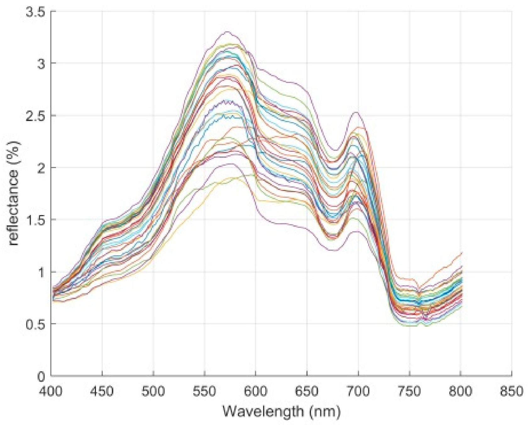
3.1. Spectral Analysis

The spectral signature of Chl-a is characterized by strong absorption in the blue (443 nm) and red wavelengths (near 675 nm), and by high reflectance in the green (550–555 nm) and red-edge spectrum regions (685–710 nm) [42,43,44,45]. Existing studies have shown that the most suitable spectral range for monitoring suspended solids in water is 700–800nm [46]. Therefore, the 181 bands with 400 to 800 nm were used for the determination of water constituents in this study. The band ratio method can eliminate background noise and rough water surface interference, and can enhance the fine spectrum characteristics that are beneficial for water quality parameter estimation [47]. This study used the band ratio method to preprocess the original spectrum. The exhaustive method was used to calculate the ratio of the bands. To identify and select the major wavelengths for the estimation of water quality parameters’ concentration, we conducted the Pearson correlation analysis.

The spectral curves of the 33 samples in the preprocessed UAV-borne hyperspectral remote sensing imagery are shown in Figure 2. The correlation coefficient between the raw spectral data and the Chl-a concentration value was negative, ranging from 0 to −0.7952. The 84 spectral absolute correlation coefficients were greater than 0.7, which were mainly concentrated in the 400–590 nm wavelength range. The correlation coefficient between the raw spectral data and the SS concentration values ranged from 0.1755 to 0.7685. The 46 spectral correlation coefficients were greater than 0.7, which were mainly concentrated in the 700~800 nm wavelength range.

This study calculated the ratio of 181 bands of the original spectra by using the exhaustive method and obtained 32580 characteristic variables. The correlation coefficients between the characteristic variables and the Chl-a concentration values ranged from −0.8196 to 0.8243. There were 12 ratio variable correlation coefficients greater than 0.81. These variables’ spectra were mainly concentrated in the 400~480 nm wavelength range. The band ratio preprocessing method improves the absorption valley characteristics of the original Chl-a spectral. The correlation of processed spectra is significantly improved compared to that of the original spectra. The correlation coefficients between the characteristic variables and the SS concentration values ranged from −0.7653 to 0.7823. There were 43 ratio variable correlation coefficients greater than 0.76. These variables’ spectra were mainly concentrated in the 592~606 nm wavelength range. When compared to the raw spectra, the correlation of the processed spectra is considerably enhanced.

3.2. Hyperparameters for the Machine Learning Algorithms

The model performance is influenced by its hyperparameters when estimating the concentration of water quality parameters. Tuning the hyperparameters is a critical step before the quantitative inversion. The key adjusting hyperparameters and their optimal parameter values for each model are shown in

Table 2. Tuned hyperparameters and their settings for each model in the prediction of Chl-a.

Models	Hyperparameters	Meanings	Search Ranges	Optimal Values
CBR	Learning rate	Shrinkage coefficient of each tree	(0.01,1)	0.26
	Max depth	Maximum depth of a tree	(1,10)	4
	Estimators	Number of trees	(100,1000)	140
	L2_leaf_reg	L2 regularization	(1,10)	7
ABR	Learning rate	Shrinkage coefficient of each tree	(0.01,0.1)	0.1
	Estimators	Number of trees	(0,200)	90
XGBR	Learning rate	Shrinkage coefficient of each tree	(0.01,1)	0.1
	Max depth	Maximum depth of a tree	(1,10)	5
	Estimators	Number of trees	(10,100)	40
	Subsample	Subsample ratio of training samples	(0.1,0.9)	0.8
GBRT	Learning rate	Shrinkage coefficient of each tree	(0.010.1)	0.05
	Estimators	Number of trees	(10,200)	150
	Subsample	Subsample ratio of training samples	(0.5,0.8)	0.5
RF	Estimators	Number of trees	(1,100)	70
	Min samples split	Minimum number of samples for nodes’ split	(1,10)	2
ERT	Max depth	Maximum depth of a tree	(1,10)	6
	Estimators	Number of trees	(0,300)	200
SVR	C	Regularization parameter	(10,200)	10
	Gamma	Kernel coefficient	(0.001,0.1)	1
MLPR	Hidden layer size	The number of neurons in the ith hidden layer and the number of hidden layers	(21), (210)	(22)
EN	Alpha	The constant of the mixed penalty term	(0.0001,0.001,0.01,0.1,1,10)	0.1

and

Table 3. Tuned hyperparameters and their settings for each model in the prediction of SS.

Models	Hyperparameters	Meanings	Search Ranges	Optimal Values
CBR	Learning rate	Shrinkage coefficient of each tree	(0.01,1)	0.1
	Max depth	Maximum depth of a tree	(1,10)	7
	Estimators	Number of trees	(100,1000)	190
	L2_leaf_reg	L2 regularization	(1,30)	26
ABR	Learning rate	Shrinkage coefficient of each tree	(0.01,0.1)	0.02
	Estimators	Number of trees	(0,200)	120
XGBR	Learning rate	Shrinkage coefficient of each tree	(0.01,1)	0.05
	Max depth	Maximum depth of a tree	(1,10)	2
	Estimators	Number of trees	(100,1000)	200
GBRT	Learning rate	Shrinkage coefficient of each tree	(0.01,0.1)	0.04
	Estimators	Number of trees	(10,200)	100
	Subsample	Subsample ratio of training samples	(0.5,0.9)	0.8
RF	Estimators	Number of trees	(1,100)	7
	Min samples split	Minimum number of samples for nodes’ split	(1,10)	3
ERT	Max depth	Maximum depth of a tree	(1,10)	4
	Estimators	Number of trees	(10,100)	20
SVR	C	Regularization parameter	(10,200)	100
	Gamma	Kernel coefficient	(0.001,10)	1
MLPR	Hidden layer size	The number of neurons in the ith hidden layer and the number of hidden layers	(21,21), (28,28)	(23,23)
EN	Alpha	The constant of the mixed penalty term	(0.0001,0.001,0.01,0.1,1,10)	0.1

.

The number and types of hyperparameters in each model are different. Selecting key parameters of the model can reduce the training time of the model and improve the prediction efficiency of the model. Since CBR, ABR, GBRT, XGBR, RF, and ERT are all tree-based models, the number of trees seriously affects the performance of the model. Too many trees will cause over-fitting of the model and an insufficient number of trees will cause underfitting. The L₂ regularization can control the complexity of the model and reduce the generalization error. The GBRT model optimizes the subsample, which controls the random sampling ratio of each tree. If the subsample value is set too small, the result will be underfitting, thus the subsample value range was between 0.5 and 1. For the ERT model, the tree’s depth is tuned. The tree’s depth determines how the model learns the characteristics of individual samples. The more individual sample features are learned, the worse the generalization ability of the model. In the SVR model, the default radial basis function was selected as the kernel function, tuning the parameters of C and gamma, which control the trade-off between the slack variable penalty and the marginal width. For the MLPR model, we tuned the parameters of the hidden layer size, which include the number of hidden layers and the number of perceptrons contained in each hidden layer.

3.3. Retrieval Results for Different Water Quality

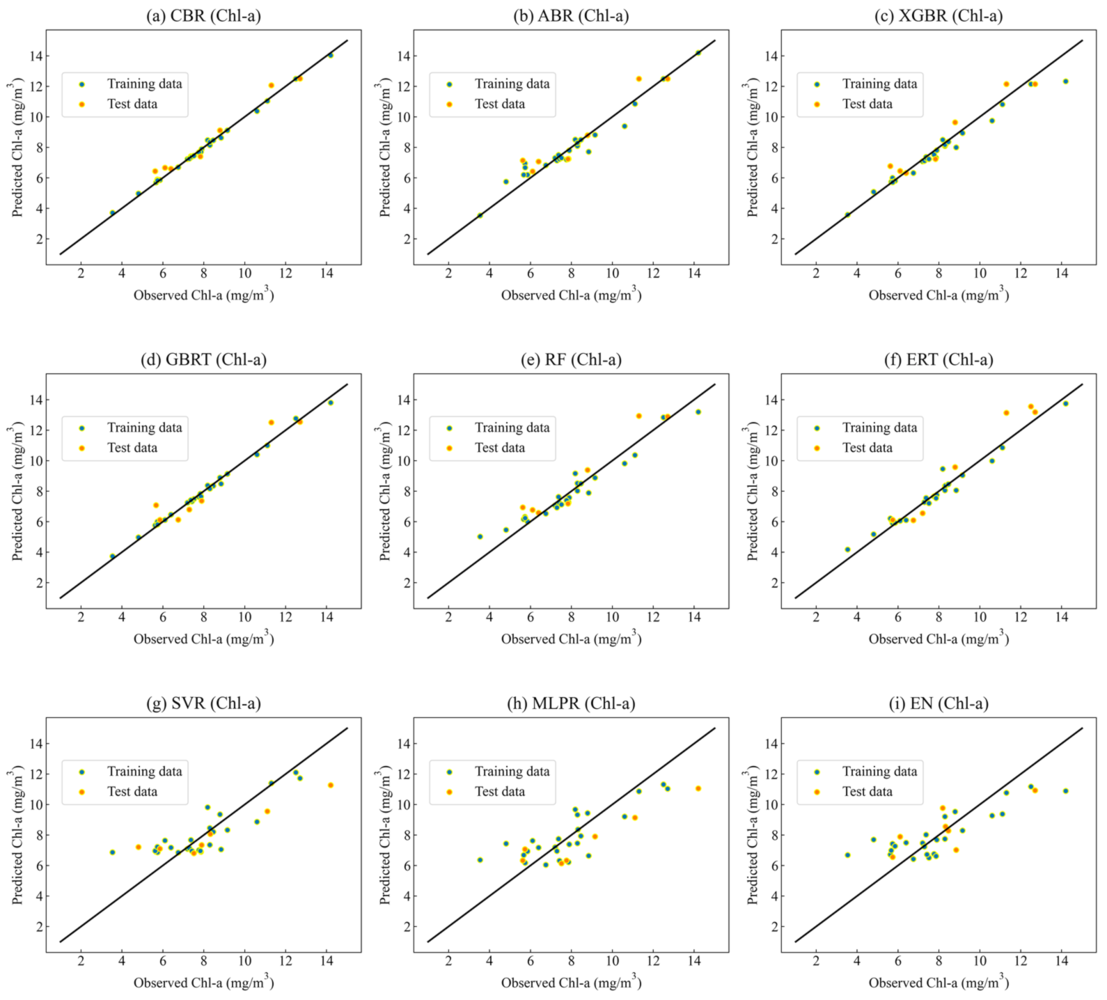
3.3.1. Retrieval Results for Chl-a

The retrieval results of each model for Chl-a are shown in

Table 4. Experimental results of Chl-a (mg/m³) using different models.

Models	Running Time (s)	Training Data Set			Test Data Set
		MAE (mg/m3)	RMSE (mg/m3)	R2	MAE (mg/m3)	RMSE (mg/m3)	R2
CBR	0.46	0.09	0.12	1.00	0.47	0.53	0.96
ABR	0.15	0.37	0.54	0.94	0.65	0.82	0.89
XGBR	0.47	0.31	0.49	0.95	0.63	0.71	0.92
GBRT	0.06	0.13	0.16	0.99	0.67	0.80	0.90
RF	0.11	0.48	0.58	0.93	0.75	0.91	0.87
ERT	0.17	0.30	0.41	0.96	0.84	0.95	0.87
SVR	0.01	0.92	1.17	0.69	1.38	1.65	0.69
MLPR	0.66	1.08	1.29	0.63	1.60	1.75	0.62
EN	0.01	1.18	1.43	0.63	1.17	1.36	0.58

. We can observe that the CBR model had the best prediction performance (R² = 0.96, MAE = 0.53 mg/m³, RMSE = 0.96 mg/m³). The prediction accuracy for the CBR validation data set (R² = 0.96, MAE = 0.53 mg/m³, RMSE = 0.96 mg/ m³) was lower than the prediction accuracy for its training data set (R² = 1.00, MAE = 0.09 mg/ m³, RMSE = 0.12 mg/m³). For the XGBR validation data set, the prediction accuracy for the XGBR model (R² = 0.92, MAE = 0.63 mg/m³, RMSE = 0.71 mg/m³) was lower than the CBR model. The prediction accuracy for the GBRT validation data set (R² = 0.90, MAE = 0.67 mg/m³, RMSE = 0.80 mg/m³) was significantly lower than the prediction accuracy for its training data set (R² = 0.99, MAE = 0.13 mg/m³, RMSE = 0.16 mg/m³). The prediction accuracy for the ABR on the training data set (R² = 0.94, MAE = 0.37 mg/m³, RMSE = 0.54 mg/m³) was also significantly higher than the prediction accuracy for its validation data set (R² = 0.89, MAE = 0.65 mg/m³, RMSE = 0.82 mg/m³). The prediction accuracy for the ERT training data set (R² = 0.96, MAE = 0.17 mg/m³, RMSE = 0.30 mg/m³) was higher than the prediction accuracy for its validation data set (R² = 0.87, MAE = 0.84 mg/m³, RMSE = 0.95 mg/m³). The prediction accuracy for the RF training data set (R² = 0.93, MAE = 0.48 mg/m³, RMSE = 0.58 mg/m³) was higher than the prediction accuracy for its validation data set (R² = 0.87, MAE = 0.75 mg/m³, RMSE = 0.91 mg/m³). The ERT model was higher than the RF model in terms of RMSE and MAE, while the ERT model and the RF model gave similar ${\mathrm{R}}^2$. The prediction performance for the SVR validation data set (R² = 0.68, MAE = 1.32 mg/m³, RMSE = 1.52 mg/m³) was comparable to the prediction performance for its training data set (R² = 0.67, MAE = 0.93 mg/m³, RMSE = 1.27 mg/m³). The prediction accuracy for the MLPR training data set (R² = 0.63, MAE = 1.08 mg/m³, RMSE = 1.29 mg/m³) was similar to the prediction accuracy for its validation data set (R² = 0.62, MAE = 1.60 mg/m³, RMSE = 1.75 mg/m³). The prediction accuracy for the EN training data (R² = 0.63, MAE = 1.18 mg/m³, RMSE = 1.43 mg/m³) was significantly decreased than the prediction accuracy for its validation data set (R² = 0.58, MAE = 1.17 mg/m³, RMSE = 1.36 mg/m³). The prediction performance of SVR, MLPR, and EN was too poor for the inversion of the concentration of Chl-a. Since these models, namely SVR, MLPR, and EN, have low R² with high MAE and RMSE, it is determined that they are not suitable for Chl-a inversion.

Scatter plots of the observed and predicted values of the nine machine learning algorithms are presented in Figure 3. The predicted and observed values of the models were evenly distributed on both sides of the regression line, indicating that the models’ prediction accuracies are excellent. The difference between the predicted values and the observed values represents the level of the model’s prediction deviation, indicating that the model may be overfitting or underfitting. From Figure 3, we can observe that the predicted values of the tree-based ensemble models, including CBR, ABR, XGBR, GBRT, RF, and ERT, were close to the regression line. Among them, the CBR, XGBR, and GBRT models have the highest prediction accuracy. The difference between the observed and the predicted values of the SVR, MLPR, and EN models is large, indicating that these models’ prediction accuracies are extremely poor.

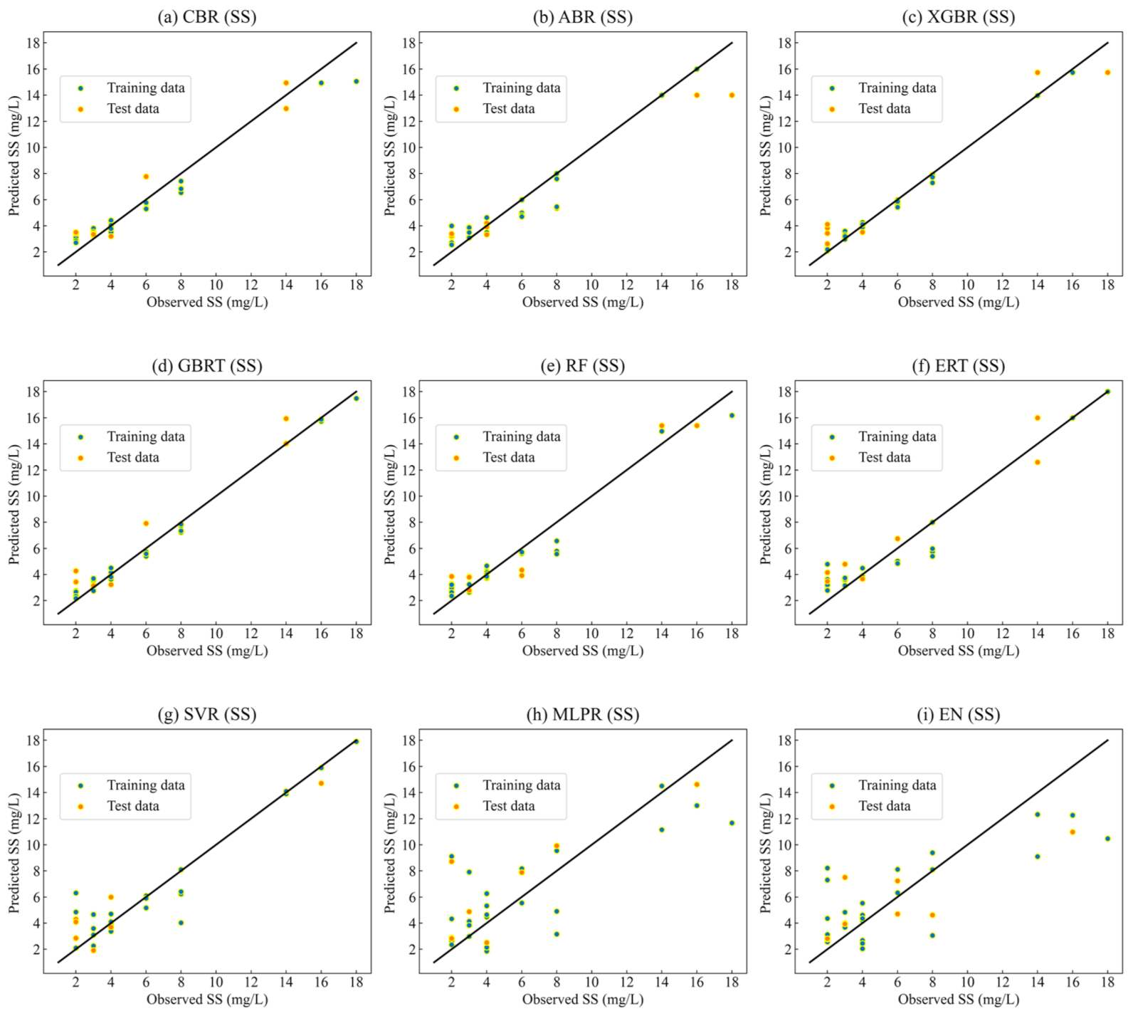
3.3.2. Retrieval Results for SS

The retrieval results of each model for SS are shown in

Table 5. Experimental results of SS (mg/L) using different models.

Models	Running Time (s)	Training Data Set			Test Data Set
		MAE (mg/L)	RMSE (mg/L)	R2	MAE (mg/L)	RMSE (mg/L)	R2
CBR	0.31	0.81	1.00	0.95	1.11	1.20	0.94
ABR	0.15	0.81	1.10	0.92	1.37	1.85	0.91
XGBR	0.51	0.22	0.29	0.99	1.50	1.64	0.93
GBRT	0.06	0.39	0.44	0.99	1.22	1.48	0.91
RF	0.02	0.86	1.11	0.93	1.23	1.39	0.93
ERT	0.03	0.85	1.17	0.93	1.41	1.54	0.90
SVR	0.12	0.84	1.44	0.90	1.42	1.57	0.89
MLPR	1.80	2.09	2.78	0.63	2.31	2.95	0.59
EN	0.01	2.12	2.91	0.60	2.46	2.97	0.55

. We can find that the CBR model had the best prediction performance (R² = 0.94, MAE = 1.11 mg/L, RMSE = 1.2 mg/L) in estimating the concentration of SS. The prediction accuracy for the CBR validation data set (R² = 0.94, MAE = 1.11 mg/L, RMSE = 1.2 mg/L) was lower than the prediction accuracy for its training data set (R² = 0.95, MAE = 0.81 mg/L, RMSE = 1 mg/L). The prediction performance for the RF validation data set (R² = 0.93, MAE = 1.23 mg/L, RMSE = 1.39 mg/L) was comparable to its training data set (R² = 0.93, MAE = 0.86 mg/L, RMSE = 1.11 mg/L). The prediction accuracy for the XGBR validation data set (R² = 0.93, MAE = 1.50 mg/L, RMSE = 1.64 mg/L) was lower than the training data set (R² = 0.99, MAE = 0.22 mg/L, RMSE = 0.29 mg/L). The prediction accuracy for the GBRT validation data set (R² = 0.91, MAE = 1.22 mg/L, RMSE = 1.48 mg/L) was significantly lower than the prediction accuracy for its training data set (R² = 0.99, MAE = 0.39 mg/L, RMSE = 0.44 mg/L). The prediction accuracy for the ABR training data set (R² = 0.91, MAE = 1.37 mg/L, RMSE = 1.85 mg/L) was similar to its validation data set (R² = 0.92, MAE = 0.81 mg/L, RMSE = 1.10 mg/L). The prediction accuracy for the ERT validation data set (R² = 0.90, MAE = 1.41 mg/L, RMSE = 1.54 mg/L) was lower than its training data set (R² = 0.93, MAE = 0.85 mg/L, RMSE = 1.17 mg/L). The prediction accuracy for the SVR validation data set (R² = 0.89, MAE = 1.42 mg/L, RMSE = 1.57 mg/L) was also lower than its training data set (R² = 0.90, MAE = 0.84 mg/L, RMSE = 1.44 mg/L). The prediction accuracy for the MLPR validation data set (R² = 0.59, MAE = 2.31 mg/L, RMSE = 2.95 mg/L) was lower than its training data set (R² = 0.63, MAE = 2.09 mg/L, RMSE = 2.78 mg/L). The prediction accuracy for the EN validation data set (R² = 0.55, MAE = 2.46 mg/L, RMSE = 2.97 mg/L) was worse than its training data set (R² = 0.60, MAE = 2.12 mg/L, RMSE = 2.91 mg/L).

Scatter plots of the observed and predicted values of CBR, ABR, XGBR, GBRT, RF, ERT, SVR, MLPR, and EN are presented in Figure 4. The scatter plots show the relationship between the predicted value of each model and the observed value. A good prediction result will be evenly distributed on both sides of the regression line. We can observe that the tree-based models’ (CBR, ABR, XGBR, GBRT, RF, ERT) predicted values and observed values were evenly distributed on both sides of the regression line, indicating that the predicted value of the model is very close to the observed value. The predicted value of the SVR model and the observed value were also evenly distributed on both sides of the regression line, and the accuracy of the SVR model was lower than that of the tree-based model. Similarly, we can observe that there was a significant difference between the predicted value and the observed value of the MLPR and EN models, indicating that the prediction errors of the MLPR and EN models are relatively large.

4. Discussion

For a further discussion, the distribution map of Chl-a obtained by CBR model for the Beigong Reservoir hyperspectral imagery is shown in Figure 5. According to the statistics of the inversion results, the maximum value of the inversion result was 14.17 mg/m³ the minimum value was 3.54 mg/m³. The observed value ranged from 2.62 mg/m³ to 14.2 mg/m³. The inversion map reveals the spatial distribution of Chl-a in the Beigong Reservoir. The concentration of Chl-a was relatively high in the west part of Beigong Reservoir and mainly concentrated along the shore.

The distribution map of SS obtained by CBR model for the Beigong Reservoir hyperspectral imagery is shown in Figure 6. According to the statistics of the inversion results, the minimum value was 2.71 mg/L and the maximum value of the inversion result was 15.04 mg/L. The observed value ranged from 2 mg/L to 18 mg/L. The inversion map shows that the SS concentration in the southwest part of the Beigong Reservoir was significantly high compared to the whole of the reservoir and there was fragmented erythema near the reservoir’s border, which may have been produced by transitory human activity.

5. Conclusions

The main purpose of this study is to compare the performance of various machine learning algorithms in predicting water quality parameters using UAV-borne hyperspectral data. Through this study, the main conclusions are as follows:

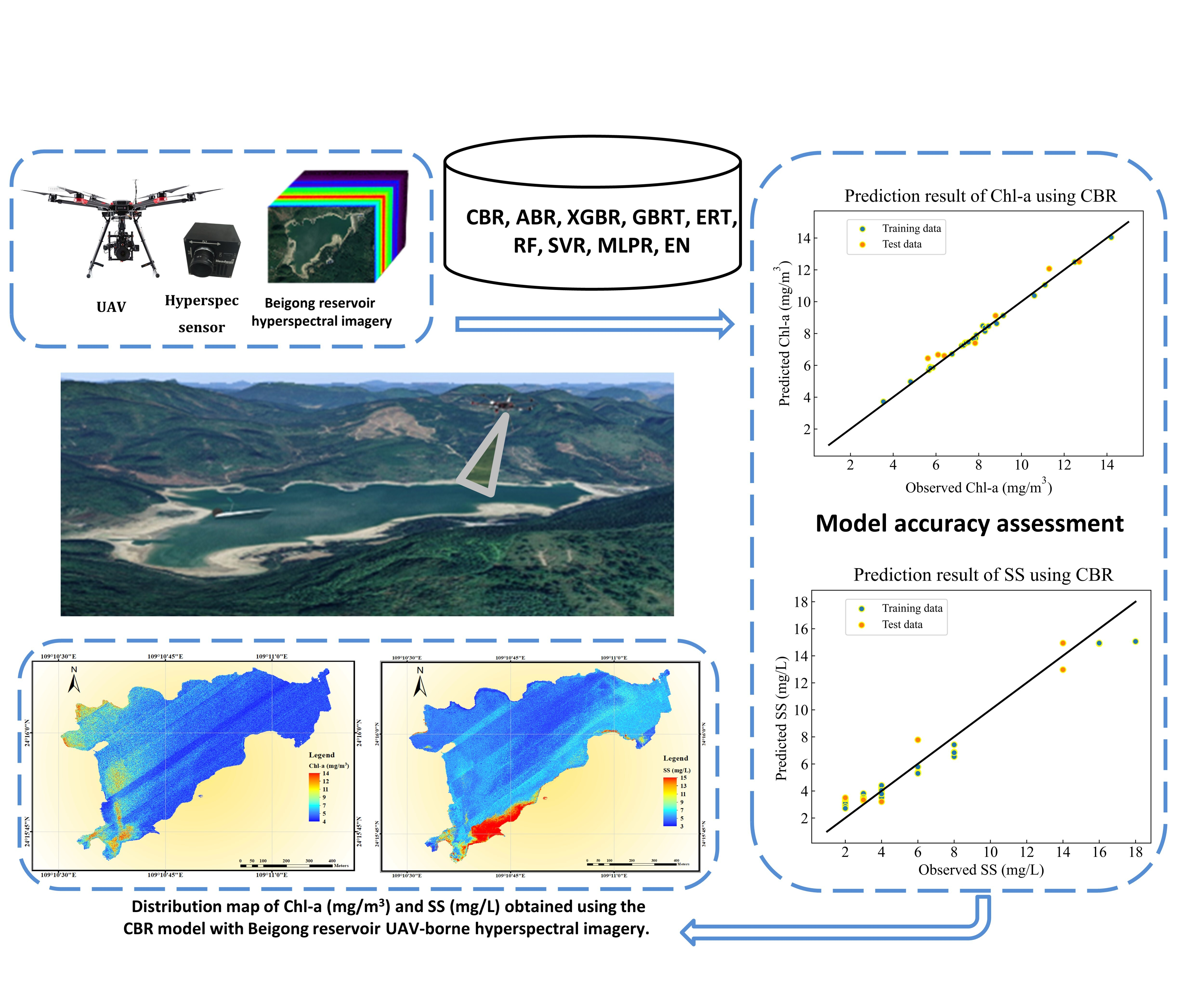
• The prediction performance of different machine learning algorithms, including CBR, XGBR, GBRT, ABR, ERT, RF, SVR, MLPR, and EN, in predicting water quality were compared. The overall prediction accuracy of the tree-based models were higher than that of the other three traditional machine learning models.
• Two water quality parameters, including Chl-a and SS, were analyzed with different machine learning models. For the prediction of Chl-a, the R² values of several models ranged from 0.58 to 0.96; the RMSE ranged from 0.53 to 1.75 mg/m³; and the MAE value ranged from 0.47 to 1.6 mg/m³. Among them, the CBR model had the highest prediction accuracy and the XGBR model had the second-highest prediction accuracy. For the prediction of SS, the R² values of the nine models ranged from 0.59 to 0.94; the RMSE ranged from 1.2 to 2.97 mg/L; and the MAE value ranged from 1.11 to 2.46 mg/L. The prediction accuracy of the CBR model was the highest and the prediction accuracies of the XGBR and RF models were lower than that of the CBR. Notably, the CBR model showed stable and satisfactory performance for predicting water quality parameters, including Chl-a and SS.
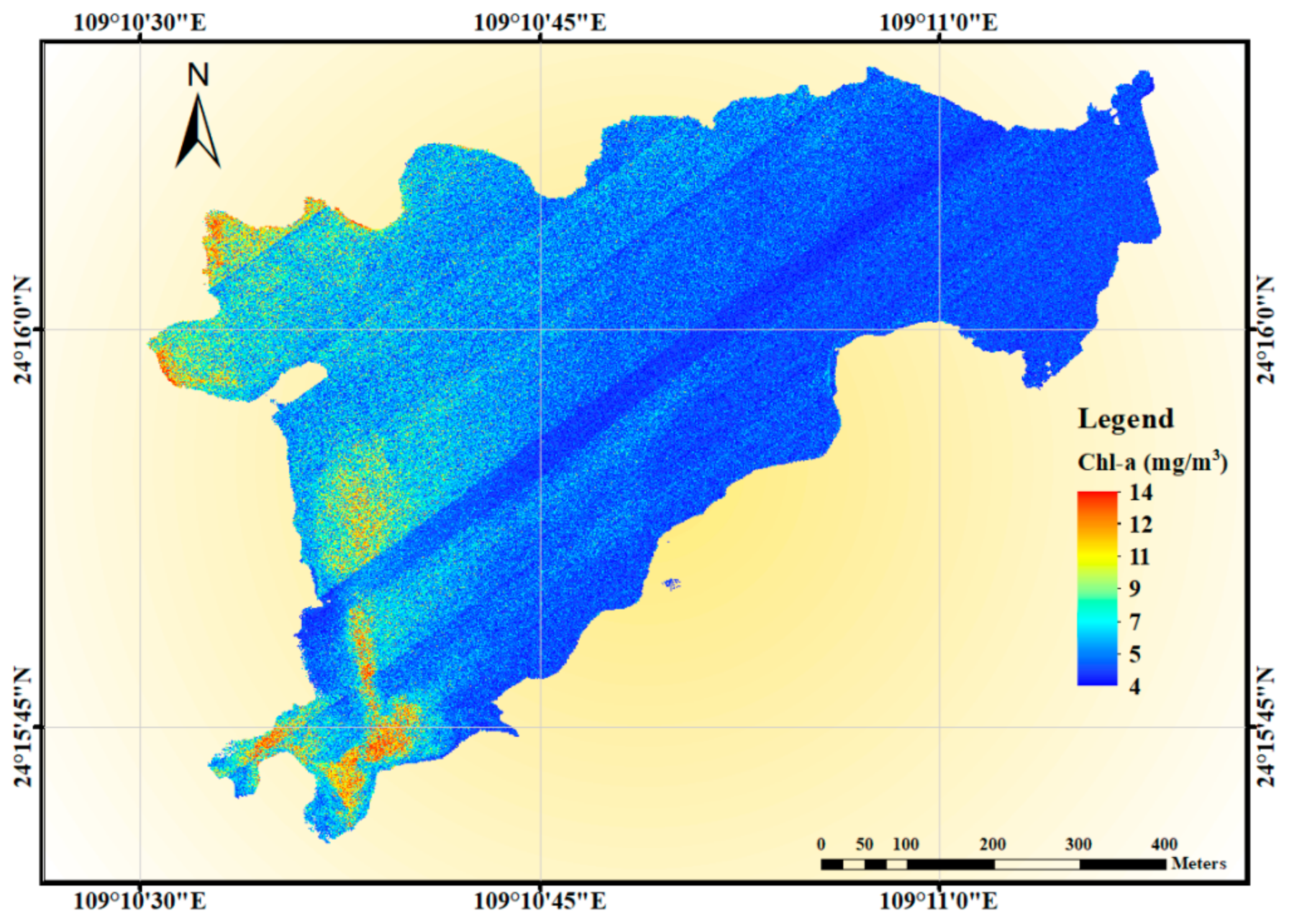
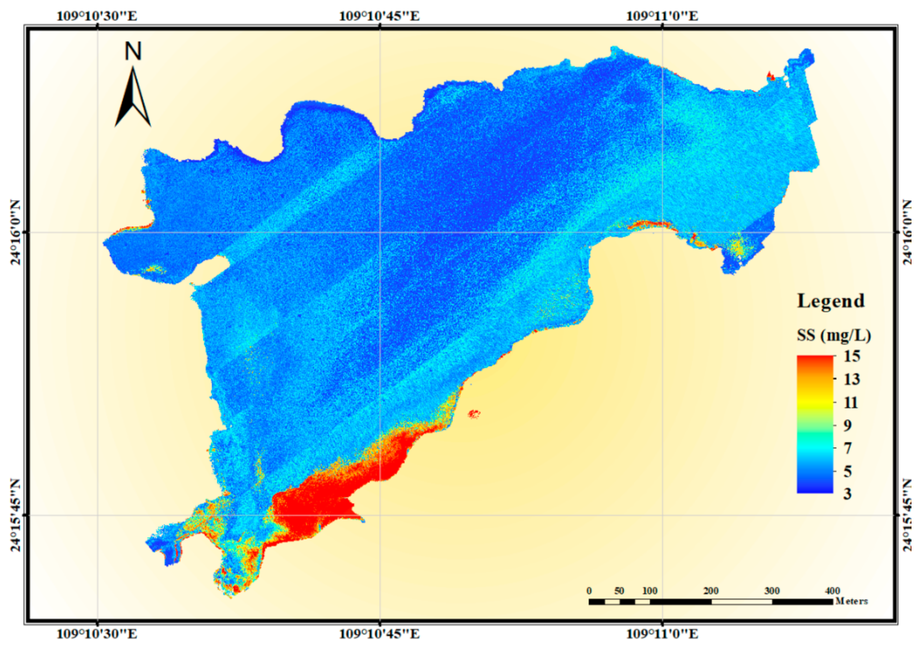
• The water quality distribution map was generated based on the UAV-borne hyperspectral data and machine learning algorithms, which can be used for large-scale and continuous inland water quality monitoring. From the water quality parameter inversion map, we observed that the pollution degree of SS in the west part of Beigong Reservoir was much higher than that in the east part. The areas with the highest Chl-a concentration mainly existed in the southern part of Beigong Reservoir and near the shore area. The management can monitor the water quality from the inversion map, improving the efficiency of water quality maintenance and saving management costs.

To conclude, this study compared and analyzed the predictive performance of nine machine learning models on different water quality parameters. In future research, we will combine multi-temporal UAV-borne hyperspectral images to analyze the dynamic change of inland water quality.

References

1. Wang, Y.; Liu, D.; Xiao, W.; Zhou, P.; Tian, C.; Zhang, C.; Du, J.; Guo, H.; Wang, B. Coastal Eutrophication in China: Trend, Sources, and Ecological Effects. Harmful Algae 2021, 107, 102058. [Google Scholar] [CrossRef] [PubMed]
2. Ding, Y.; Zhao, J.; Peng, W.; Zhang, J.; Chen, Q.; Fu, Y.; Duan, M. Stochastic Trophic Level Index Model: A New Method for Evaluating Eutrophication State. J. Environ. Manag. 2021, 280, 111826. [Google Scholar] [CrossRef] [PubMed]
3. Sun, F.; Mu, Y.; Leung, K.M.Y.; Su, H.; Wu, F.; Chang, H. China Is Establishing Its Water Quality Standards for Enhancing Protection of Aquatic Life in Freshwater Ecosystems. Environ. Sci. Policy 2021, 124, 413–422. [Google Scholar] [CrossRef]
4. Moses, W.J.; Gitelson, A.A.; Perk, R.L.; Gurlin, D.; Rundquist, D.C.; Leavitt, B.C.; Barrow, T.M.; Brakhage, P. Estimation of Chlorophyll-a Concentration in Turbid Productive Waters Using Airborne Hyperspectral Data. Water Res. 2012, 46, 993–1004. [Google Scholar] [CrossRef] [PubMed] [Green Version]
5. Birtwell, I.K.; Farrell, M.; Jonsson, A. The Validity of Including Turbidity Criteria For Aquatic Resource Protection in Land Development Guideline (Pacific and Yukon Region). In Canadian Manuscript Report of Fisheries and Aquatic Sciences; Fisheries and Oceans Canada: Ottawa, ON, Canada, 2008. [Google Scholar]
6. Bierman, P.; Lewis, M.; Ostendorf, B.; Tanner, J. A Review of Methods for Analysing Spatial and Temporal Patterns in Coastal Water Quality. Ecol. Indic. 2011, 11, 103–114. [Google Scholar] [CrossRef]
7. Huang, W.; Chen, S.; Yang, X.; Johnson, E. Assessment of Chlorophyll-a Variations in High- and Low-Flow Seasons in Apalachicola Bay by MODIS 250-m Remote Sensing. Environ. Monit. Assess. 2014, 186, 8329–8342. [Google Scholar] [CrossRef]
8. Doña, C.; Chang, N.-B.; Caselles, V.; Sánchez, J.M.; Camacho, A.; Delegido, J.; Vannah, B.W. Integrated Satellite Data Fusion and Mining for Monitoring Lake Water Quality Status of the Albufera de Valencia in Spain. J. Environ. Manag. 2015, 151, 416–426. [Google Scholar] [CrossRef] [Green Version]
9. Du, C.; Li, Y.; Wang, Q.; Liu, G.; Zheng, Z.; Mu, M.; Li, Y. Tempo-Spatial Dynamics of Water Quality and Its Response to River Flow in Estuary of Taihu Lake Based on GOCI Imagery. Environ. Sci. Pollut. Res. 2017, 24, 28079–28101. [Google Scholar] [CrossRef]
10. Syariz, M.A.; Lin, C.-H.; Nguyen, M.V.; Jaelani, L.M.; Blanco, A.C. WaterNet: A Convolutional Neural Network for Chlorophyll-a Concentration Retrieval. Remote Sens. 2020, 12, 1966. [Google Scholar] [CrossRef]
11. Rajesh, A.; Jiji, G.W.; Raj, J.D. Estimating the Pollution Level Based on Heavy Metal Concentration in Water Bodies of Tiruppur District. J. Indian Soc. Remote Sens. 2020, 48, 47–57. [Google Scholar] [CrossRef]
12. Rostom, N.G.; Shalaby, A.A.; Issa, Y.M.; Afifi, A.A. Evaluation of Mariut Lake Water Quality Using Hyperspectral Remote Sensing and Laboratory Works. Egypt. J. Remote. Sens. Space Sci. 2017, 20, S39–S48. [Google Scholar] [CrossRef] [Green Version]
13. Quan, Q.; Hao, Z.; Xifeng, H.; Jingchun, L. Research on Water Temperature Prediction Based on Improved Support Vector Regression. Neural Comput. Appl. 2020. [Google Scholar] [CrossRef]
14. Leong, W.C.; Bahadori, A.; Zhang, J.; Ahmad, Z. Prediction of Water Quality Index (WQI) Using Support Vector Machine (SVM) and Least Square-Support Vector Machine (LS-SVM). Int. J. River Basin Manag. 2021, 19, 149–156. [Google Scholar] [CrossRef]
15. Lu, H.; Ma, X. Hybrid Decision Tree-Based Machine Learning Models for Short-Term Water Quality Prediction. Chemosphere 2020, 249, 126169. [Google Scholar] [CrossRef]
16. Najah Ahmed, A.; Binti Othman, F.; Abdulmohsin Afan, H.; Khaleel Ibrahim, R.; Ming Fai, C.; Shabbir Hossain, M.; Ehteram, M.; Elshafie, A. Machine Learning Methods for Better Water Quality Prediction. J. Hydrol. 2019, 578, 124084. [Google Scholar] [CrossRef]
17. Sharafati, A.; Asadollah, S.B.H.S.; Hosseinzadeh, M. The Potential of New Ensemble Machine Learning Models for Effluent Quality Parameters Prediction and Related Uncertainty. Process. Saf. Environ. Prot. 2020, 140, 68–78. [Google Scholar] [CrossRef]
18. Parsimehr, M.; Shayesteh, K.; Godini, K.; Bayat Varkeshi, M. Using Multilayer Perceptron Artificial Neural Network for Predicting and Modeling the Chemical Oxygen Demand of the Gamasiab River. Avicenna J. Environ. Health Eng. 2018, 5, 15–20. [Google Scholar] [CrossRef]
19. Xiaojuan, L.; Mutao, H.; Jianbao, L. Remote Sensing Inversion of Lake Water Quality Parameters Based on Ensemble Modelling. E3S Web Conf. 2020, 143, 02007. [Google Scholar] [CrossRef]
20. Tang, J.W.; Tian, G.L.; Wang, X.Y.; Wang, X.M.; Song, Q.J. The Methods of Water Spectra Measurement and Analysis I: Above-Water Method. J. Remote. Sens. 2004, 8, 37–44. [Google Scholar]
21. Mobley, C.D. Estimation of the Remote-Sensing Reflectance from above-Surface Measurements. Appl. Opt. AO 1999, 38, 7442–7455. [Google Scholar] [CrossRef] [PubMed]
22. Kelcey, J.; Lucieer, A. Sensor Correction of a 6-Band Multispectral Imaging Sensor for UAV Remote Sensing. Remote. Sens. 2012, 4, 1462–1493. [Google Scholar] [CrossRef] [Green Version]
23. Qun’ou, J.; Lidan, X.; Siyang, S.; Meilin, W.; Huijie, X. Retrieval Model for Total Nitrogen Concentration Based on UAV Hyper Spectral Remote Sensing Data and Machine Learning Algorithms—A Case Study in the Miyun Reservoir, China. Ecol. Indic. 2021, 124, 107356. [Google Scholar] [CrossRef]
24. He, J.; Lin, J.; Ma, M.; Liao, X. Mapping Topo-Bathymetry of Transparent Tufa Lakes Using UAV-Based Photogrammetry and RGB Imagery. Geomorphology 2021, 389, 107832. [Google Scholar] [CrossRef]
25. Zhang, Y.; Wu, L.; Ren, H.; Liu, Y.; Zheng, Y.; Liu, Y.; Dong, J. Mapping Water Quality Parameters in Urban Rivers from Hyperspectral Images Using a New Self-Adapting Selection of Multiple Artificial Neural Networks. Remote Sens. 2020, 12, 336. [Google Scholar] [CrossRef] [Green Version]
26. Wang, X.; Xie, S.; Zhang, X.; Chen, C.; Guo, H.; Du, J.; Duan, Z. A Robust Multi-Band Water Index (MBWI) for Automated Extraction of Surface Water from Landsat 8 OLI Imagery. Int. J. Appl. Earth Obs. Geoinf. 2018, 68, 73–91. [Google Scholar] [CrossRef]
27. Campos, J.C.; Sillero, N.; Brito, J.C. Normalized Difference Water Indexes Have Dissimilar Performances in Detecting Seasonal and Permanent Water in the Sahara–Sahel Transition Zone. J. Hydrol. 2012, 464–465, 438–446. [Google Scholar] [CrossRef]
28. Ying, H.; Xia, K.; Huang, X.; Feng, H.; Yang, Y.; Du, X.; Huang, L. Evaluation of Water Quality Based on UAV Images and the IMP-MPP Algorithm. Ecol. Inform. 2021, 61, 101239. [Google Scholar] [CrossRef]
29. Wei, L.; Huang, C.; Zhong, Y.; Wang, Z.; Hu, X.; Lin, L. Inland Waters Suspended Solids Concentration Retrieval Based on PSO-LSSVM for UAV-Borne Hyperspectral Remote Sensing Imagery. Remote Sens. 2019, 11, 1455. [Google Scholar] [CrossRef] [Green Version]
30. Freund, Y. Boosting a Weak Learning Algorithm by Majority; AT&T Laboratories: Murray Hill, NJ, USA, 1995. [Google Scholar]
31. Freund, Y.; Schapire, R.E. A Decision-Theoretic Generalization of On-Line Learning and an Application to Boosting. J. Comput. Syst. Sci. 1997, 55, 119–139. [Google Scholar] [CrossRef] [Green Version]
32. Friedman, J.H. Greedy Function Approximation: A Gradient Boosting Machine. Ann. Stat. 2001, 29, 1189–1232. [Google Scholar] [CrossRef]
33. Chen, T.; Guestrin, C. XGBoost: A Scalable Tree Boosting System. In Proceedings of the 22nd ACM SIGKDD International Conference on Knowledge Discovery and Data Mining, Association for Computing Machinery. New York, NY, USA, 13 August 2016; pp. 785–794. [Google Scholar]
34. Dong, W.; Huang, Y.; Lehane, B.; Ma, G. XGBoost Algorithm-Based Prediction of Concrete Electrical Resistivity for Structural Health Monitoring. Autom. Constr. 2020, 114, 103155. [Google Scholar] [CrossRef]
35. Dorogush, A.V.; Ershov, V.; Gulin, A. CatBoost: Gradient Boosting with Categorical Features Support. arXiv 2018, arXiv:1810.11363. [Google Scholar]
36. Breiman, L. Random Forests. Mach. Learn. 2001, 45, 5–32. [Google Scholar] [CrossRef] [Green Version]
37. Geurts, P.; Ernst, D.; Wehenkel, L. Extremely Randomized Trees. Mach. Learn 2006, 63, 3–42. [Google Scholar] [CrossRef] [Green Version]
38. Cheng, H.; Shi, Y.; Wu, L.; Guo, Y.; Xiong, N. An Intelligent Scheme for Big Data Recovery in Internet of Things Based on Multi-Attribute Assistance and Extremely Randomized Trees. Inf. Sci. 2021, 557, 66–83. [Google Scholar] [CrossRef]
39. Raghavendra, N.S.; Deka, P.C. Support Vector Machine Applications in the Field of Hydrology: A Review. Appl. Soft Comput. 2014, 19, 372–386. [Google Scholar] [CrossRef]
40. Günther, F.; Fritsch, S. Neuralnet: Training of Neural Networks. R J. 2010, 2, 30. [Google Scholar] [CrossRef] [Green Version]
41. Zou, H.; Hastie, T. Regression Shrinkage and Selection via the Elastic Net, with Applications to Microarrays. JR Stat. Soc. Ser. B 2004, 67, 301–320. [Google Scholar] [CrossRef] [Green Version]
42. He, J.; Chen, Y.; Wu, J.; Stow, D.A.; Christakos, G. Space-Time Chlorophyll-a Retrieval in Optically Complex Waters That Accounts for Remote Sensing and Modeling Uncertainties and Improves Remote Estimation Accuracy. Water Res. 2020, 171, 115403. [Google Scholar] [CrossRef] [PubMed]
43. Beck, R.; Zhan, S.; Liu, H.; Tong, S.; Yang, B.; Xu, M.; Ye, Z.; Huang, Y.; Shu, S.; Wu, Q.; et al. Comparison of Satellite Reflectance Algorithms for Estimating Chlorophyll-a in a Temperate Reservoir Using Coincident Hyperspectral Aircraft Imagery and Dense Coincident Surface Observations. Remote. Sens. Environ. 2016, 178, 15–30. [Google Scholar] [CrossRef] [Green Version]
44. Soomets, T.; Uudeberg, K.; Jakovels, D.; Brauns, A.; Zagars, M.; Kutser, T. Validation and Comparison of Water Quality Products in Baltic Lakes Using Sentinel-2 MSI and Sentinel-3 OLCI Data. Sensors 2020, 20, 742. [Google Scholar] [CrossRef] [PubMed] [Green Version]
45. Buma, W.G.; Lee, S.-I. Evaluation of Sentinel-2 and Landsat 8 Images for Estimating Chlorophyll-a Concentrations in Lake Chad, Africa. Remote Sens. 2020, 12, 2437. [Google Scholar] [CrossRef]
46. Gholizadeh, M.H.; Melesse, A.M.; Reddi, L. A Comprehensive Review on Water Quality Parameters Estimation Using Remote Sensing Techniques. Sensors 2016, 16, 1298. [Google Scholar] [CrossRef] [PubMed] [Green Version]
47. Huang, M.; Kim, M.S.; Delwiche, S.R.; Chao, K.; Qin, J.; Mo, C.; Esquerre, C.; Zhu, Q. Quantitative Analysis of Melamine in Milk Powders Using Near-Infrared Hyperspectral Imaging and Band Ratio. J. Food Eng. 2016, 181, 10–19. [Google Scholar] [CrossRef] [Green Version]
Figure 1. The study area and sampling information.
Remotesensing 13 03928 g001
Figure 2. The spectral curves of the 33 samples in the preprocessed UAV-borne hyperspectral remote sensing imagery.
Remotesensing 13 03928 g002
Figure 3. Scatter plot of the observed values and predicted values of Chl-a concentration (mg/m3) using nine machine learning models including CBR, ABR, XGBR, GBRT, RF, ERT, SVR, MLPR, and EN.
Remotesensing 13 03928 g003
Figure 4. Scatter plot of the observed values and the predicted values of the SS (mg/L) concentration using nine machine learning models including CBR, ABR, XGBR, GBRT, RF, ERT, SVR, MLPR, and EN.
Remotesensing 13 03928 g004
Figure 5. Distribution map of Chl-a (mg/m3) obtained using the CBR model with Beigong UAV-borne hyperspectral imagery.
Remotesensing 13 03928 g005
Figure 6. Distribution map of SS (mg/L) obtained using the CBR model with Beigong UAV-borne hyperspectral imagery.
Remotesensing 13 03928 g006