Drought Assessment in the São Francisco River Basin Using Satellite-Based and Ground-Based Indices

Abstract

The São Francisco River Basin (SFRB) plays a key role for the agricultural and hydropower sectors in Northeast Brazil (NEB). Historically, in the low part of the SFRB, people have to cope with strong periods of drought. However, there are incipient signs of increasing drought conditions in the upper and middle parts of the SFRB, where its main reservoirs (i.e., Três Marias, Sobradinho, and Luiz Gonzaga) and croplands are located. Therefore, the assessment of the impacts of extreme drought events in the SFRB is of vital importance to develop appropriate drought mitigation strategies. These events are characterized by widespread and persistent dry conditions with long-term impacts on water resources and rain-fed agriculture. The purpose of this study is to provide a comprehensive evaluation of extreme drought events in terms of occurrence, persistence, spatial extent, severity, and impacts on streamflow and soil moisture over different time windows between 1980 and 2020. The Standardized Precipitation-Evapotranspiration Index (SPEI) and Standardized Streamflow Index (SSI) at 3- and 12-month time scales derived from ground data were used as benchmark drought indices. The self-calibrating Palmer Drought Severity Index (scPDSI) and the Soil Moisture and Ocean Salinity-based Soil Water Deficit Index (SWDIS) were used to assess the agricultural drought. The Water Storage Deficit Index (WSDI) and the Groundwater Drought Index (GGDI) both derived from the Gravity Recovery and Climate Experiment (GRACE) were used to assess the hydrological drought. The SWDISa and WSDI showed the best performance in assessing agricultural and hydrological droughts across the whole SFRB. A drying trend at an annual time scale in the middle and south regions of the SFRB was evidenced. An expansion of the area under drought conditions was observed only during the southern hemisphere winter months (i.e., JJA). A marked depletion of groundwater levels concurrent with an increase in soil moisture content was observed during the most severe drought conditions, indicating an intensification of groundwater abstraction for irrigation. These results could be useful to guide social, economic, and water resource policy decision-making processes.

1. Introduction

Drought is one of the most important extreme events that threatens food and water security in many parts of the world [1], especially in developing countries and particularly in Brazil [2,3]. With the advent of climate change, the severity, duration, and spatial extent of droughts are projected to increase in some Brazilian regions, such as the São Francisco River Basin (SFRB) [4,5]. The SFRB plays an important role in supplying water for human consumption, agricultural irrigation, and hydropower production in Northeast Brazil (NEB) [6], which is a vast region marked by socioeconomic disparities and high societal vulnerability to drought [7,8].

Over the past years, the SFRB has been experiencing more frequent and extreme drought events [9,10,11]. Numerous studies conducted in this basin show that the occurrence of extreme and severe meteorological drought events is linked to distinct climate systems modulated by El Niño–Southern Oscillation (ENSO) conditions [11], sea surface temperature (SST) anomalies in the tropical Atlantic [12], Pacific Decadal Oscillation (PDO) [13], or to an interaction of these indices at different time scales [10,13,14]. This situation carries serious implications for the agriculture and hydroelectric sectors, such as those observed between 2012 and 2015 [13]. Furthermore, it threatens the sustainability and economic viability of the water transfer project from the São Francisco River to the semiarid NEB [15]. This water infrastructure project aims to improve water security for more than 12 million people in the semiarid region of the NEB [16]. In this context, there is a need for a comprehensive exploration of this natural hazard and a deeper understanding on their spatial distribution to support the development of strategies of planning and managing water resources during drought and water scarcity conditions.

Drought is classified into four major types: meteorological, hydrological, agricultural, and socioeconomic drought [17]. A prolonged deficit of precipitation corresponds to meteorological drought [18]. When the deficit is persistent in time and begins to negatively impact crops it is referred to as an agricultural drought [19]. Hydrological drought often occurs after the onset of meteorological drought, and is characterized by abnormally low streamflow in rivers and abnormally low levels in lakes, reservoirs, and groundwater [20]. Socioeconomic drought refers to conditions in which the water supply cannot satisfy the demand related to human activities [21].

The simplest way for monitoring drought conditions is to use standardized drought indices which are derived from observed measurements such as precipitation, soil moisture, streamflow, and groundwater levels [17]. They aim to categorize and quantify droughts in terms of the severity, duration, and spatial extent [22]. Despite the wide variety of available drought indices [22,23], they have limitations when applied to large regions with scarce ground-based data because the local features of the drought cannot be generalized [22]. However, in recent years, the increased availability of satellite missions dedicated to earth observation have allowed the calculation of various drought indices using remote sensing data, modeled data, and merged data to overcome this problem in data scarce regions [24,25,26,27,28].

Although the SFRB is a region where observed measurements are scarce, very few studies have used satellite-based drought indices to assess the impacts of drought in this basin. For example, Santos et al. [29] used the SPI at different time scales derived from Tropical Rainfall Measuring Mission (TRMM) to investigate the spatiotemporal behavior of meteorological droughts in the SFRB. They found that the southwest and south/southeast parts of the basin have been the most affected by droughts in term of drought event severity between January 1998 and December 2013. Su et al. [11] assessed the spatiotemporal extent of the 2012–2015 drought event in the SFRB by using GRACE-derived TWS fields. They pointed out that the SFRB experienced a water linear depletion rate of 27.63 km³/year during 02/2012–01/2015. Nevertheless, as far as we know, there is no recent study that assesses the interaction between the different types of droughts in the SFRB. In light of this, meaningful value will be added to the literature on the large-scale impact of drought in the SFRB through state-of-the-art satellite-based drought indices.

Some drought indices commonly used for drought assessment include the Standardized Precipitation Evapotranspiration Index (SPEI) [30], Soil Water Deficit Index (SWDI) [31], self-calibrating Palmer Drought Severity Index (scPDSI) [32], Standardized Streamflow Index (SSI) [33], Water Storage Deficit Index (WSDI) [34], and Groundwater Drought Index (GGDI) [35], among others.

The SPEI has been widely used to monitor meteorological drought impacts in different parts of the world due to its multi-scalar nature and its sensitivity to long-term temperature variability [30]. It is similar to the Standardized Precipitation Index (SPI) in the way in which it is calculated, but the SPEI is based on a simplified climatic water balance (precipitation (P) minus potential evapotranspiration (PET)) computed at different time scales [36] and normalized with a log-logistic probability distribution function to remove the seasonal effect [37]. Therefore, the SPEI is better suited than the SPI for evaluating the impacts of drought under global climate change [36].

The scPDSI has been used for identifying and monitoring agricultural droughts [22]. It is based on a simple two-layer bucket soil moisture balance in the rooting zone where the soil water capacity, precipitation, and PET are used as inputs. The calculation of the scPDSI includes a self-calibrating procedure by replacing its empirical constants with dynamically calculated values based on the characteristics of the local climate [32]. The SWDI is a relatively new agricultural drought index, which is based on the ratio of the difference between soil moisture and field capacity and the difference between field capacity and wilting point [38]. Because the SWDI is independent of record length, it has been applied for operational monitoring of agricultural drought integrating surface soil moisture estimates from the Soil Moisture and Ocean Salinity (SMOS) mission [7,39].

The SSI is a hydrological drought index based on the same theoretical basis as the SPI [22]. It is used to characterize anomalies in observed streamflow data at different time scales [40,41]. Moreover, the WSDI and GGDI are hydrological drought indices [42]. Unlike the SSI, the WDSI and GGDI are derived from the Gravity Recovery and Climate Experiment (GRACE) satellite missions and are applicable to study large-scale terrestrial water storage (TWS) changes [34,35]. Each of the abovementioned drought indices has strengths, weaknesses, and limitations. Hence, in order to have a complete picture of drought features in a region, the integration of several drought indices is needed [22].

This work aims to analyze the concomitant impacts between the different types of droughts in order to understand their short-term and long-term characteristics in the entire SFRB. The major novelty of this study with respect to similar previous studies is the use of the latest version of the GRACE, SMOS-based soil moisture, and satellite-based scPDSI datasets together with high-quality ground-based data to delineate those areas of the SFRB where drought events are becoming more frequent and persistent.

2. Materials and Methods

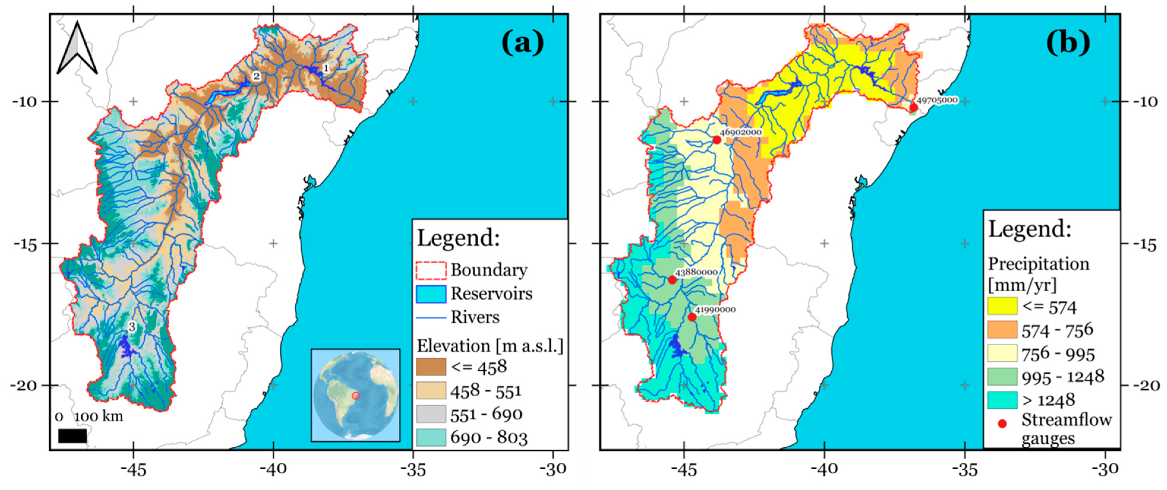
2.1. Study Area

The study was carried out over the SFRB, which is located between 7.2–21.1° S and 36.3–47.6° W (Figure 1a), with a drainage area of 621,812 km² at the basin outlet and an annual mean discharge of 1961 m³/s at Propriá on its mainstream [43]. The SFRB has approximately 14 million inhabitants (71.7 4 inhabitants per square kilometer) distributed among seven states: Bahia, Minas Gerais, Pernambuco, Alagoas, Sergipe, Goiás, and part of the Federal District [44]. Its mainstream is 2696 km long [10], starting in the Serra da Canastra (Minas Gerais) and reaching the Atlantic Ocean between the border of Alagoas and Sergipe. The main reservoirs are Três Marias, Sobradinho, and Itaparica (Luíz Gonzaga), whose useful reservoir volumes are 15,278 hm³, 28,669 hm³, and 3549 hm³, respectively [45]. Roughly 68% of the SFRB climate is Aw (tropical with wet summers and dry winters) according to the Köppen–Geiger type-climate classification [46]. The mean annual temperature in the SFRB is approximately 24 °C, ranging from 18 °C in the more elevated areas of the Serra da Canastra to 27 °C in the northern lowlands [47]. The mean annual precipitation across the SFRB is around 910 mm, ranging from around 400 mm to >1500 mm [10] (Figure 1b). The temporal variability of precipitation is largely modulated by SST anomalies over the tropical Atlantic region and the ENSO phenomenon [12,48]. Over the middle SFRB, the rainy season occurs during November to January, and from January to March in the northern basin [10]. The elevation of the SFRB gradually rises from the northern lowlands (near the mouth of the São Francisco River) to the Serra da Canastra (above 1800 m above sea level (a.s.l.)). The cropland is the most prominent land cover in the SFRB and covers about 44% of its entire surface [49], with 6,902,960 ha devoted to irrigated annual crops such as soybean, wheat, and maize in 2017 [50].

2.2. Datasets

2.2.1. Ground-Based Data

Precipitation and Potential Evapotranspiration Data

P and PET were derived from a gridded product (version 2.0) developed by Xavier et al. [52] using ground-based climate data provided by the Brazilian Water Agency (ANA), the National Institute of Meteorology (INMET), and the Water and Electric Energy Department of São Paulo state (DAEE). The PET is based on the Food and Agriculture Organization of the United Nations-56 (FAO-56) Penman–Monteith formulation [53]. The procedure to generate this product involved a quality control and homogeneity check. Further information on the generation and validation of this dataset can be found at Xavier et al. [54]

Streamflow Data

Daily streamflow time series were obtained from the Brazilian National Water Agency (ANA). Propriá, Várzea da Palma, Boqueirão, and Santo Inácio were selected as reliable benchmark streamflow gauges (see Figure 1b) because they exhibit less than 3% missing data per month. To verify whether the daily streamflow time series are stationary, the Augmented Dickey–Fuller (ADF) test was computed omitting the missing observations as shown in Ryan and Giles [55]. All time series were stationary at the 5% significance level (Supplementary Material Table S1). Hence, missing data were filled using autoregressive integrated moving average (ARIMA) models with the lowest Akaike Information Criterion (AIC) and Bayesian Information Criterion (BIC) values through the R package imputeTS (version 3.2; Moritz and Bartz-Beielstein [56]).

2.2.2. Satellite-Based Data

SMOS Surface Soil Moisture Data

SMOS is an L-band passive microwave satellite dedicated to global surface soil moisture (SSM, top 0–5 cm) monitoring [57]. For this study, the SSM estimates were extracted from the SMOS L3 SSM product (version 3.0) provided by the Barcelona Expert Center. This product was averaged considering its ascending and descending orbits to minimize the influence of the radio frequency interference (RFI) on retrieved SSM values [58]. The choice of this product was based on its acceptable performance in the identification of agricultural drought when compared to in situ measurements in the SFRB [7,59].

GRACE/GRACE-FO Data

The GRACE twin-satellite mission and its follow-on (GRACE-Follow-On) is a joint mission of the National Aeronautics and Space Administration (NASA) and the German Aerospace Center (DLR) that measures the surface mass changes which, in turn, are related to the terrestrial water storage anomalies (TWSA) [60]. The TWSA integrates snowpack water equivalent, canopy water storage, surface water storage, soil moisture storage, and groundwater storage relative to a time baseline [61]. The GRACE/GRACE-FO-derived TWSA products developed by the Center for Space Research at the University of Texas (CSR v2.0; [62]), the German Research Center for Geoscience (GFZ v3; [63]), and the Jet Propulsion Laboratory (JPL v2; [64]) were used. To minimize the noise and systematic errors from different products [65], they were resampled using the nearest neighbor technique to 1° × 1° and then averaged in each grid point [11]. The stationarity of the averaged TWSA time series was verified with the ADF test [55] on a per-pixel basis. Since the TWSA time series were stationary (Supplementary Material Figure S1), the data gaps in all GRACE/GRACE-FO products (i.e., caused by satellite batteries and accelerometer failure; [42]) were filled using ARIMA models. The AIC and BIC values were used as goodness-of-fit measures. The TWSA data are relative to the baseline mean over January 2004 to December 2009 (except the GFZ product, which is referred to during the period April 2002 to March 2020) [63]. Therefore, for comparisons against other datasets used in this study, a new baseline was computed by averaging each grid point from April 2002 to March 2020 and subtracting that value from all time steps [42]. The reason for choosing these products is that they have shown an acceptable performance in quantifying the impact of drought events over the SFRB through different TWSA-based drought indexes [11,66].

2.3. Drought Indices

2.3.1. Ground-Based Drought Indices

Standardized Precipitation Evapotranspiration Index (SPEI)

The SPEI was used to assess meteorological drought conditions and their variability in time. For the calculation of the SPEI, P and PET were derived from the gridded product developed by Xavier et al. [52]. In this study, the aggregation of P minus PET for a set of n months, followed by standardization to zero mean and unit standard deviation, is called SPEIn. Regardless of the time scale, the physical meaning of positive SPEI values is the occurrence of wetter than average conditions (i.e., water surplus), while negative values denote drier than average conditions (i.e., water deficit). This dataset provides reliable information for drought assessment in Brazil, as confirmed in previous studies [67,68,69]. The spatial and temporal consistency of the SPEI was checked and their area-averaged time series were visually inspected to detect any problems before use. In this study, the SPEI was adopted as a benchmark drought index because of its traceable feature. The SPEI at 3- and 12-month time scales was calculated using the R package SPEI (version 1.7; Vicente-Serrano et al. [30]). The reference period for computing SPEI was 01/1980 to 12/2015. The rationale behind the choice of the SPEI is related to the fact that it is appropriate to assess meteorological droughts in the context of global warming due to its high sensibility to temperature changes [70]. The 3- and 12-month time scales were selected to focus attention on both short-term (i.e., SPEI3) and long-term (i.e., SPEI12) drought events. For more details about the mathematical basis of the SPEI, see Vicente-Serrano et al. [30].

Standardized Streamflow Index (SSI)

Understanding the role of the propagation of meteorological droughts into hydrological droughts on recent droughts over the SFRB is a relevant topic. The SSI was used to identify the occurrence and the intensity of hydrological droughts and its propagation on some reaches of the São Francisco River. For its calculation at 3- and 12-month time scales (i.e., SSI3 and SSI12), daily streamflow time series obtained from the ANA were used. The motivation behind the use of SSI came out of its good performance in the characterization of hydrological drought events over the NEB [71]. More details about the theoretical background of SSI can be found in Tijdeman et al. [72].

2.3.2. Satellite-Based Drought Indices

SMOS-Based Soil Water Deficit Index (SWDIS)

In this study, the SWDIS was used to assess the impact of drought conditions on SSM. The SWDIS was proposed by Martínez-Fernández et al. [31] as follows:

$$\mathrm{SWDIS}=10\left(\frac{\mathsf{\theta }-{\mathsf{\theta }}_{\mathrm{FC}}}{{\mathsf{\theta }}_{\mathrm{AWC}}}\right)$$

(1)

where θ is the soil water content derived from SMOS-based SSM time series (m³/m³) FC denotes field capacity (m³/m³), and AWC available water content (m³/m³), which is the difference between FC and WP (wilting point). The 5th and 95th percentiles derived from SMOS-based SSM time series were used as estimators of WP and FC, respectively [73]. For calculation of the monthly SWDIS at each SMOS pixel, the SSM estimates were extracted from the SMOS L3 SSM product. To remove the seasonal signal, the SWDIS time series were standardized by removing the climatology mean and dividing by standard deviation (SWDISa). Thus, positive SWDISa values indicate greater-than-mean SWDIS (excess moisture), while negative values indicate less-than-mean SWDIS (deficit moisture). Further details of the SWDIS can be found in Martínez-Fernández et al. [31].

Self-Calibrating Palmer Drought Severity Index (scPDSI)

In order to assess the impact of drought conditions on the plant root zone soil moisture (i.e., 0–100 cm), a global scPDSI dataset was used [32]. It was obtained from the Climatic Research Unit (CRU) of University of East Anglia, who used the fields of monthly precipitation (P) and temperature (T) registers available in the CRU high-resolution surface climate data set (CRU TS) as inputs in its calculation [74]. For this study, a subset of this dataset spanning 1981 to 2020 with monthly resolution was used. The rationale behind the choice of this dataset is related to the fact that the scPDSI has a high sensitivity to agricultural drought in the NEB [71], has moderate spatial resolution, and that it was recently updated by the CRU (version 4.05). More details and information on the scPDSI can be found at van der Schrier et al. [74].

Water Storage Deficit Index (WSDI)

Once the TWSA monthly time series over the SRFB was obtained, the WSDI was computed in each grid point as proposed by Thomas et al. [34]:

$${\mathrm{WSD}}_{\mathrm{i},\mathrm{j}}={\mathrm{TWSA}}_{\mathrm{i},\mathrm{j}}-\overline{{\mathrm{TWSA}}_{\mathrm{i}}}$$

(2)

$$\mathrm{WSDI}=\frac{\mathrm{WSD}-\mathsf{\mu }}{\mathsf{\sigma }}$$

(3)

where WSD is the Water Storage Deficit [dimensionless] for the month i (from 1 to 12) and the year j (from 2002 to 2020); TWSA_i,j represents the value of TWSA [cm] for the i month and the j year; and $\overline{\mathrm{TWSA}}$_i the long-term mean for all values of TWSA [cm] at the i month. The obtained time series of WSD in each grid point was normalized by its long-term mean (µ) and standard deviation (σ), resulting in the WSDI (Equation (3)). Further details about the WSDI are presented by Nigatu et al. [42].

GRACE-Based Groundwater Drought Index (GGDI)

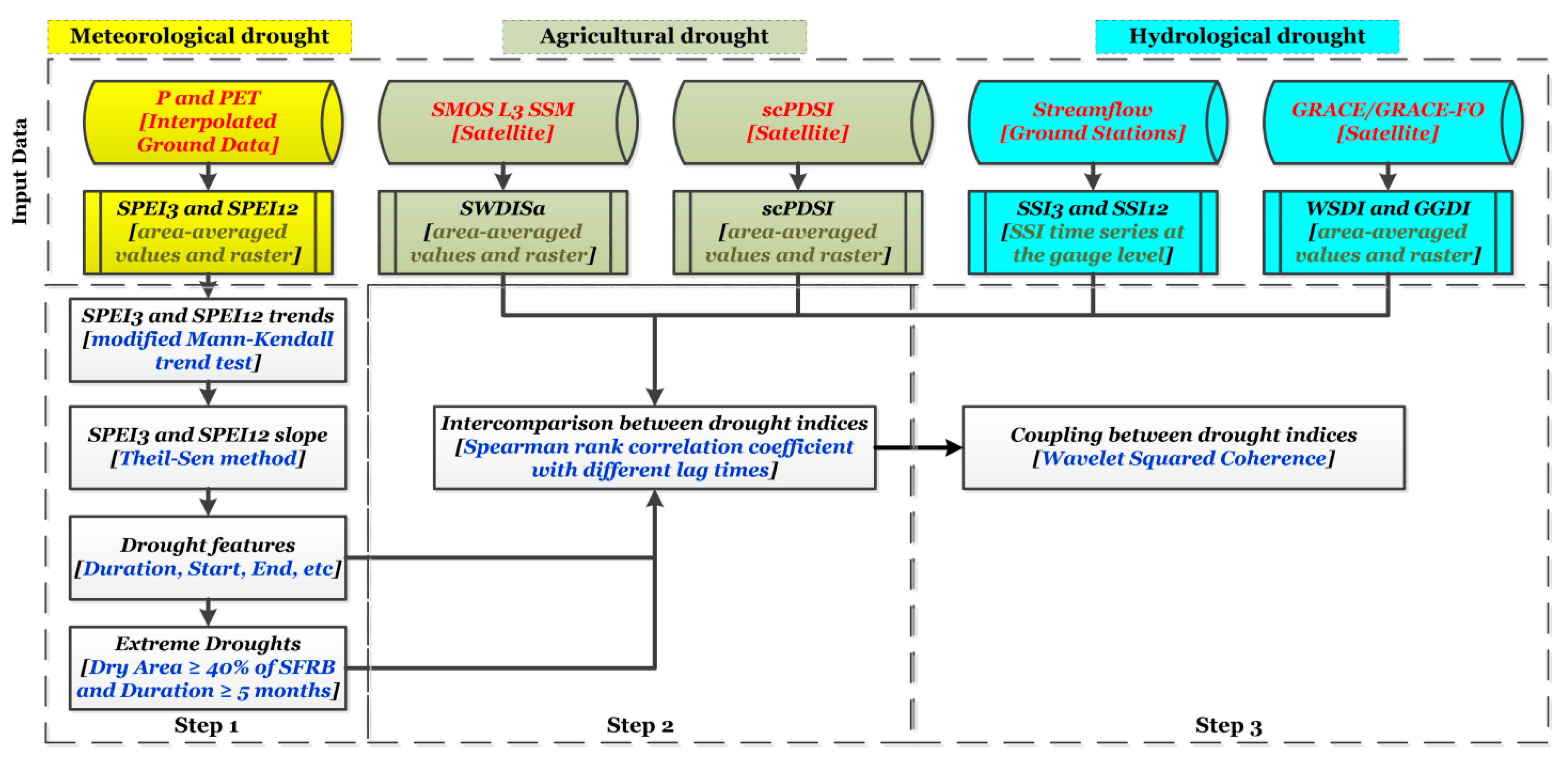
Since drought can affect groundwater storage in the SFRB [75], the GGDI developed by Wang et al. [76] was implemented to investigate the spatiotemporal characteristics of groundwater drought. Firstly, the groundwater storage anomalies changes (GWSAΔ) were computed by subtracting the incremental change of the snowpack water equivalent anomalies (SWEAΔ), canopy water storage anomalies (CWSAΔ), surface water storage anomalies (SWSAΔ), and soil moisture storage anomalies (SMSAΔ) from the changes of GRACE-based TWSA (TWSAΔ) according to the Equations (4)–(8).

$$\mathrm{GWSA}\mathsf{\Delta }=\mathrm{TWSA}\mathsf{\Delta }-\left(\mathrm{SWEA}\mathsf{\Delta }-\mathrm{CWSA}\mathsf{\Delta }-\mathrm{SWSA}\mathsf{\Delta }-\mathrm{SMSA}\mathsf{\Delta }\right)$$

(4)

$$\mathrm{TWSA}\mathsf{\Delta }={\mathrm{TWSA}}_{\mathrm{i}}-{\mathrm{TWSA}}_{\mathrm{i}-1}$$

(5)

$$\mathrm{SWEA}\mathsf{\Delta }={\mathrm{SWEA}}_{\mathrm{i}}-{\mathrm{SWEA}}_{\mathrm{i}-1}$$

(6)

$$\mathrm{CWSA}\mathsf{\Delta }={\mathrm{CWSA}}_{\mathrm{i}}-{\mathrm{CWSA}}_{\mathrm{i}-1}$$

(7)

$$\mathrm{SWSA}\mathsf{\Delta }={\mathrm{SWSA}}_{\mathrm{i}}-{\mathrm{SWSA}}_{\mathrm{i}-1}$$

(8)

where TWSA_i (SWEA_i, CWSA_i, and SWSA_i) is the TWSA (SWEA, CWSA, and SWSA) [cm] for the i month; and TWSA_i−1 signifies the value of TWSA (SWEA, CWSA, and SWSA) [cm] for the i − 1 month between April 2002 and March 2020.

The SWE, CWS, and SMS were extracted from the Global Land Data Assimilation System (GLDAS) Noah Land Surface Model L4 monthly v2.1 dataset [77]. The SWS was calculated using TerraClimate data [78]. For consistency, the SWE, CWS, SMS, and SWS were resampled through the nearest neighbor technique to match the 1° × 1° grid of GRACE-based TWSA. Then, these variables were converted to monthly anomalies (i.e., SWEA, CWSA, SMSA, and SWSA) considering the baseline period April 2002 to March 2020 (i.e., as with the GRACE-based TWSA). Secondly, the time series of GWSAΔ was normalized subtracting the climatology mean for the i month (from 1 to 12) and all j years (from 2002 to 2020), and then dividing by their standard deviation (sd) to remove seasonality in the time series of GWSAΔ as suggested by Nigatu et al. [42], resulting in the GGDI (equation 9). Similar to the WSDI, this processing was applied to each TWSA grid point.

Table 1. Summary of the drought indices used in this study.

Drought Index	Product/Data Name	Time Period	Temporal Resolution	Spatial Resolution	Data Source	Accessed on
SPEI	P	01/1980 to 12/2015	Monthly	0.25°	https://bit.ly/2QyPvbm	15 Jan 2021
	PET	01/1980 to 12/2015	Monthly	0.25°	https://bit.ly/2QyPvbm	15 Jan 2021
SWDIS	SMOS L3 SSM (asc)	06/2010 to 03/2020	Monthly	0.225°	http://bec.icm.csic.es	10 Feb 2021
	SMOS L3 SSM (des)	06/2010 to 03/2020	Monthly	0.225°	http://bec.icm.csic.es	10 Feb 2021
scPDSI	CRU TS-based P	01/1981 to 12/2020	Monthly	0.5°	https://bit.ly/3v8sUl1	10 Jun 2021
	CRU TS-based T	01/1981 to 12/2020	Monthly	0.5°	https://bit.ly/3v8sUl1	10 Jun 2021
SSI	Streamflow	01/1980 to 03/2020	Daily	---	https://bit.ly/3vb2LSn	10 Jun 2021
WSDI and GGDI	GRACE-based CSR v2.0	04/2002 to 03/2020	Monthly	0.25°	https://bit.ly/3bOqNeg	04 Aug 2021
	GRACE-based GFZ v3	04/2002 to 03/2020	Monthly	1°	https://bit.ly/2Sm2ldE	04 Aug 2021
	GRACE-based JPL v2	04/2002 to 03/2020	Monthly	0.5°	https://grace.jpl.nasa.gov	04 Aug 2021
GGDI	GLDAS Noah Model	04/2002 to 03/2020	Monthly	0.25°	https://disc.gsfc.nasa.gov	04 Aug 2021
	TerraClimate	04/2002 to 03/2020	Monthly	1/24°	https://bit.ly/3c550iL	04 Aug 2021

summarizes the datasets employed in this study.

$$\mathrm{GGDI}=\frac{\mathrm{GWSA}{\mathsf{\Delta }}_{\mathrm{i},\mathrm{j}}-{\overline{\mathrm{GWSA}\mathsf{\Delta }}}_{\mathrm{i}}}{\mathrm{sd}(\mathrm{GWSA}{\mathsf{\Delta }}_{\mathrm{i}})}$$

(9)

2.4. Methodology

The study involved three steps in sequence. In the first step, the seasonal and annual SPEI trends at 3- and 12-month time scales were studied to determine whether there have been any significant changes in meteorological drought trends from 1980 to 2015. To do so, the modified Mann–Kendall trend test was applied to the area-averaged time series of SPEI3 and SPEI12 via the mean. This is a non-parametric test widely used to verify the presence of long-term trends in time series regardless of the existence of serial correlation [79,80]. The threshold levels of statistical significance to identify a monotonic trend were 5% (p value ≤ 0.05, high statistical significance) and 10% (0.05 < p value ≤ 0.10, moderate statistical significance), with the null hypothesis of no trend. The Theil–Sen method was used to compute the slope of said trends [81]. Furthermore, to calculate the spatial characteristics of this type of drought the following criteria were applied at each grid point. A dry spell starts when SPEI ≤ −1.00 for at least two consecutive months, and it ends when SPEI > −1.00. These thresholds were adopted to focus attention on the drought categories referred to as moderate dry, severe dry, and extremely dry (

Table 2. Drought categories for the values of SPEI, SSI, SWDISa, scPDSI, WSDI, and GGDI.

Drought Category	SPEI/SSI	Probability [%] 1	SWDISa	scPDSI	WSDI	GGDI
Extreme wet	>2.00	84.14	>0.44	>4.00	>0.96	>0.62
Severe wet	1.50 to 1.99	81.86	0.34 to 0.44	4.00 to 3.00	0.84 to 0.96	0.52 to 0.62
Moderate wet	1.00 to 1.49	77.45	0.23 to 0.33	2.99 to 2.00	0.64 to 0.83	0.33 to 0.51
Near normal	0.99 to −0.99	68.27	0.24 to −0.82	1.99 to −1.99	0.63 to −1.30	0.32 to −1.08
Moderate dry	−1.00 to −1.49	9.18	−0.83 to −1.15	−2.00 to −2.99	−1.31 to −1.49	−1.09 to −1.34
Severe dry	−1.50 to −1.99	4.41	−1.16 to −1.27	−3.00 to −3.99	−1.50 to −1.67	−1.35 to −1.49
Extreme dry	<−2.00	2.28	<−1.28	<−4.00	<−1.68	<−1.50

¹ The cumulative probability of non-exceedance for each SPEI/SSI drought category according to Junqueira et al. [83].

), which can trigger severe impacts on agriculture and hydroelectric sectors in the SFRB. The duration of a dry spell is the number of months between its onset and end. The intensity is the minimum SPEI value during the occurrence of a dry spell. The severity of a drought event is the absolute value of the sum of the values of SPEI from the beginning to end of said drought event. For a given month, the drought spatial coverage is the percentage of pixels with values of SPEI ≤ −1.00. For this study, seven meteorological drought categories were considered according to the criteria proposed by McKee et al. [82], as shown in Table 2.

A comprehensive analysis of the extreme drought events in the SFRB was also carried out. The approach adopted considers that they occur when the drought spatial coverage is greater than 40% for at least five consecutive months. During these episodes, the temporal persistence was assessed. In this study, this refers to the time period (as a percentage of the duration of the extreme drought event) in which a pixel shows values of SPEI ≤ −1.00 [84]. Under this condition, significant impacts on the surface soil moisture and the root zone, streamflow, and reservoir and groundwater levels would be expected. Based on this premise, in a second step, the linear association between the area-averaged values of SPEI3 and SPEI12 against SWDISa, scPDSI, SSI3, SSI12, WSDI, and GGDI during their coincident time periods was analyzed. To that end, the Spearman rank correlation coefficient was considered. In order to make the Spearman correlation analysis more reliable, all time series were previously detrended using linear regression for removing trend and seasonal components [85]. The use of this statistical measure was motivated by the fact that it does not require normally distributed data and can be interpreted as the Pearson coefficient [86]. To perform a consistent comparison between the drought indices categories, seven drought categories equivalent to the corresponding values of SPEI3 were developed considering the same cumulative probability of non-exceedance in each SPEI drought category for the corresponding quantiles in the area-averaged time series of SWDISa, WSDI, and GGDI during their common period (see Table 2). The scPDSI was classified following the categories proposed by Well et al. [32]

Droughts exhibit non-stationary properties due to their association with different large-scale oceanic-climatic drivers (e.g., ENSO) in the SFRB [11,87]. Therefore, in a third step, we applied a wavelet squared coherence (WSC) analysis to reveal underlying oscillation patterns and changes in periodicities in a time-frequency domain between the area-averaged values of SPEI against SWDISa, scPDSI, SSI, WSDI, and GGDI during their common time periods. These time series were previously detrended using linear regression to remove the effects of any underlying trend and seasonal components [85]. The WSC is defined as the absolute value squared of a smoothed cross-wavelet spectrum, normalized by the smoothed wavelet power (more details in Labat et al. [88]). The computational procedure of the WCA described by Torrence and Compo [89] was used. The Monte Carlo approach was used in the estimation of the level of statistical significance [90]. Both metrics were calculated through the R package biwavelet (version 0.20.21) developed by Gouhier et al. [91]. The rationale behind the use of the WSC is that it has been recognized as a robust statistical approach to evaluate the coupling between different drought indices where multiple underlying oscillations are present [13,88,92]. For the sake of clarity, Figure 2 provides the overall picture of the methodology used in the study.

3. Results

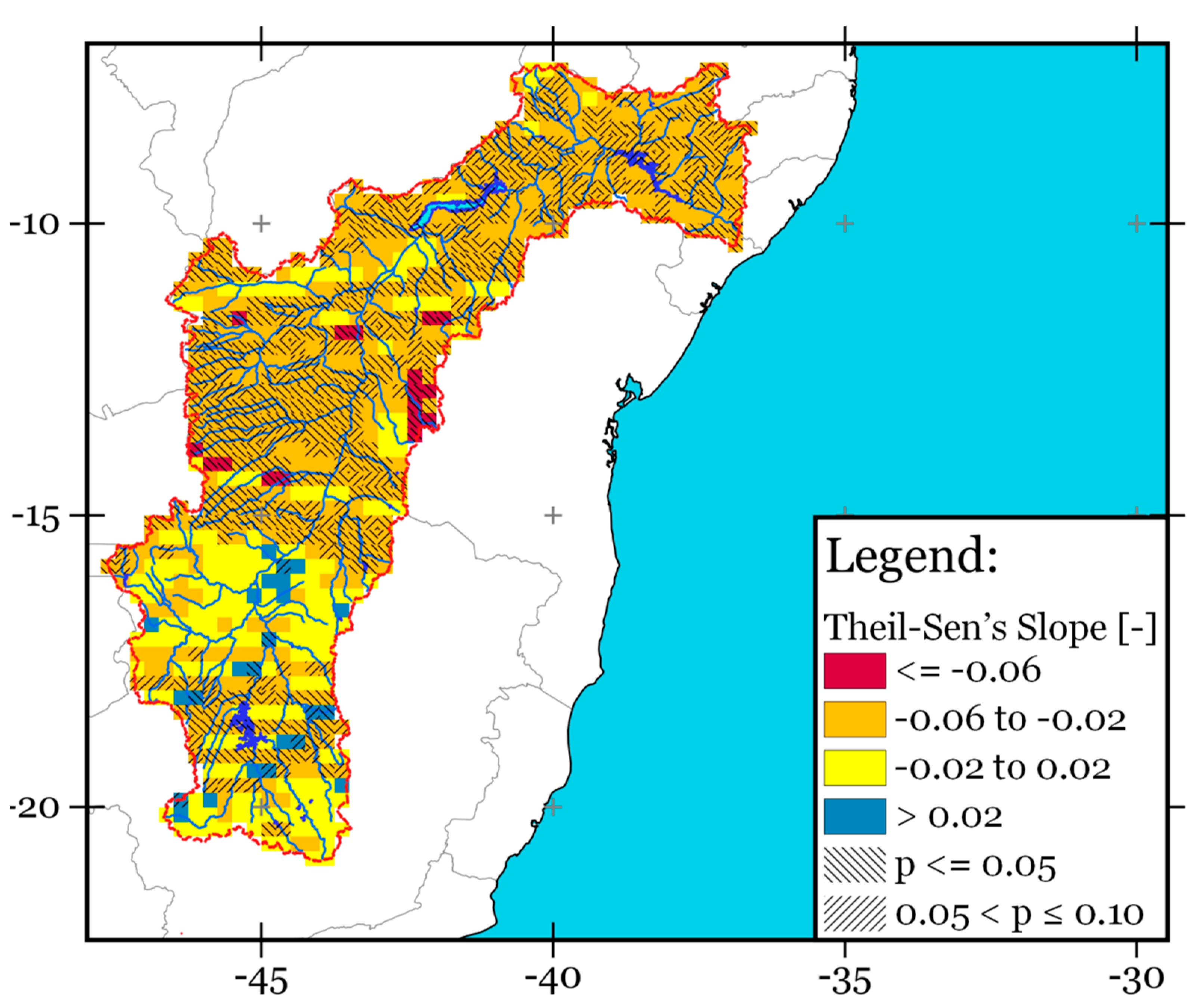
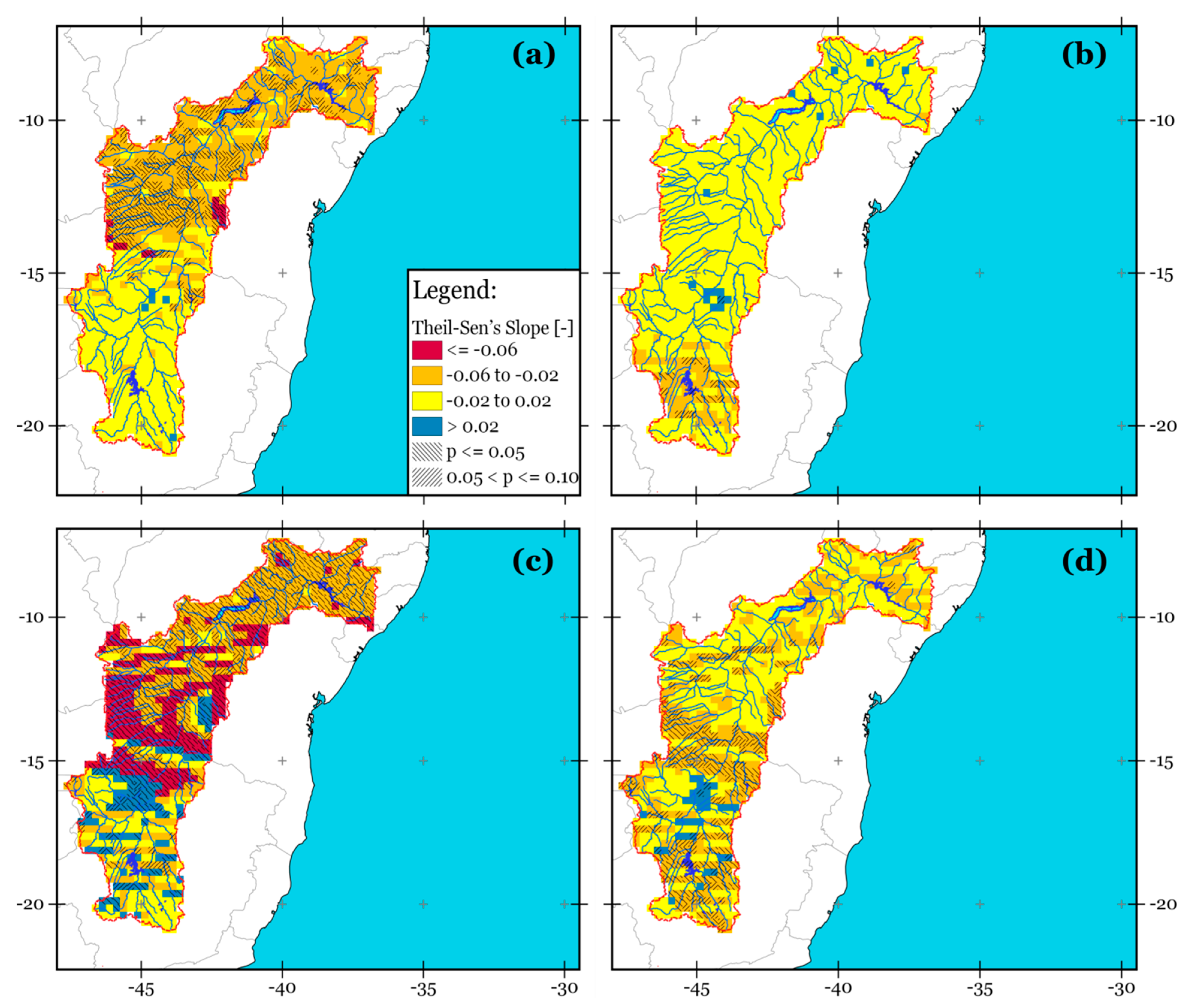
3.1. Spatial–Temporal Trends of SPEI3 and SPEI12

The SPEI12 at December (hereinafter SPEI12-December) uses as input the cumulative precipitation from January to December for each year. Therefore, it is sensitive to interannual variability of precipitation. Figure 3 shows the spatial–temporal trend of SPEI12-December over the SFRB during the period 1980–2015. The values of SPEI12-December with significant Theil–Sen’s slope shown in orange and red indicate the dominance of drying trends at annual time scale, whereas ones shown in blue indicate the dominance of wetting trends. Around 37% of the SFRB experienced a significant drying trend (p ≤ 0.05) concentrated in the middle and south regions of the basin, while 17% showed a possible drying trend (0.05 < p value ≤ 0.10). The more intensive drying trend with high statistical significance (Theil–Sen’s slope < –0.06 and p ≤ 0.05) occurred on the upper part of the Paramirim River sub-basin near the Serra do Espinhaço (roughly 7000 km²).

Unlike the SPEI12, the SPEI3 takes into account the cumulative precipitation for three consecutive months. For this reason, it serves as a reasonable proxy to evaluate the long-term trend of seasonal droughts. Based on this premise, the SPEI3 was chosen in order to characterize the seasonal trend of the climatic water balance (i.e., Precipitation - Potential Evapotranspiration) over the SFRB. In terms of trends of SPEI3-February (DJF), -May (MAM), -August (JJA), and -November (SON) for each year and during 1980–2015, a strong drought exacerbation (significant at 95% confidence level) in the middle and southern sub-basins during the June–July–August (JJA) and December–January–February (DJF) seasons was observed (Figure 4a,c). Overall, 59% of the SFRB showed a significant drying trend (p ≤ 0.05) during the JJA season, while for the DJF, SON, and MAM seasons it was 16%, 14%, and 1%. For the SON and MAM seasons, although a predominant drying trend was evident (Figure 4b,d), it was only significant over some regions of middle SFRB and the major tributaries of the Três Marias reservoir in the Minas Gerais State (see Figure 1a). DJF is the main rainfall season in the basin so its failure often triggers a shortage of water in the NEB [10,18].

These results indicate the occurrence of a long-term drying trend (p ≤ 0.05) over a large portion of the SFRB throughout the 1980–2015 period, particularly in the JJA season. To gain further insights on the drying trend, the temporal variation of the area under drought conditions was analyzed.

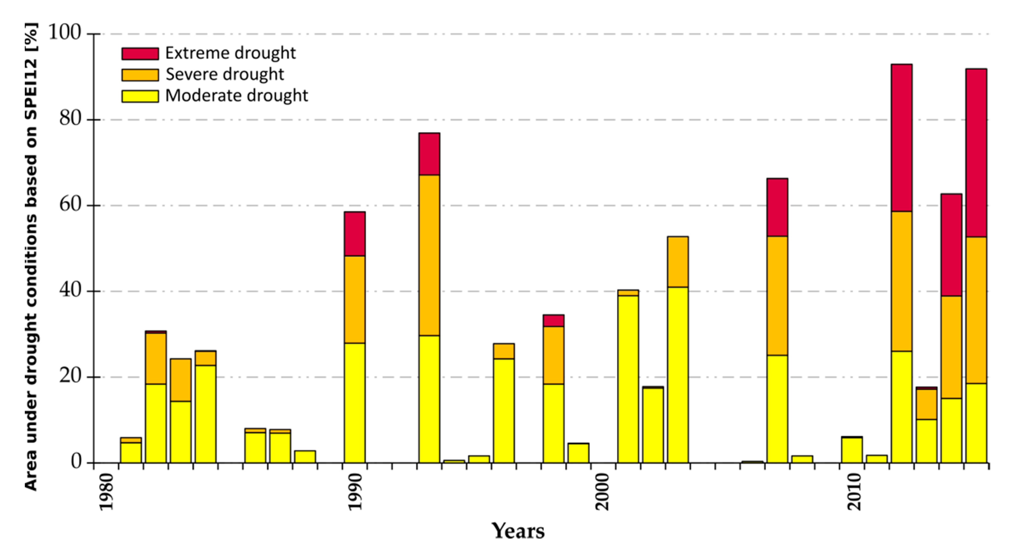
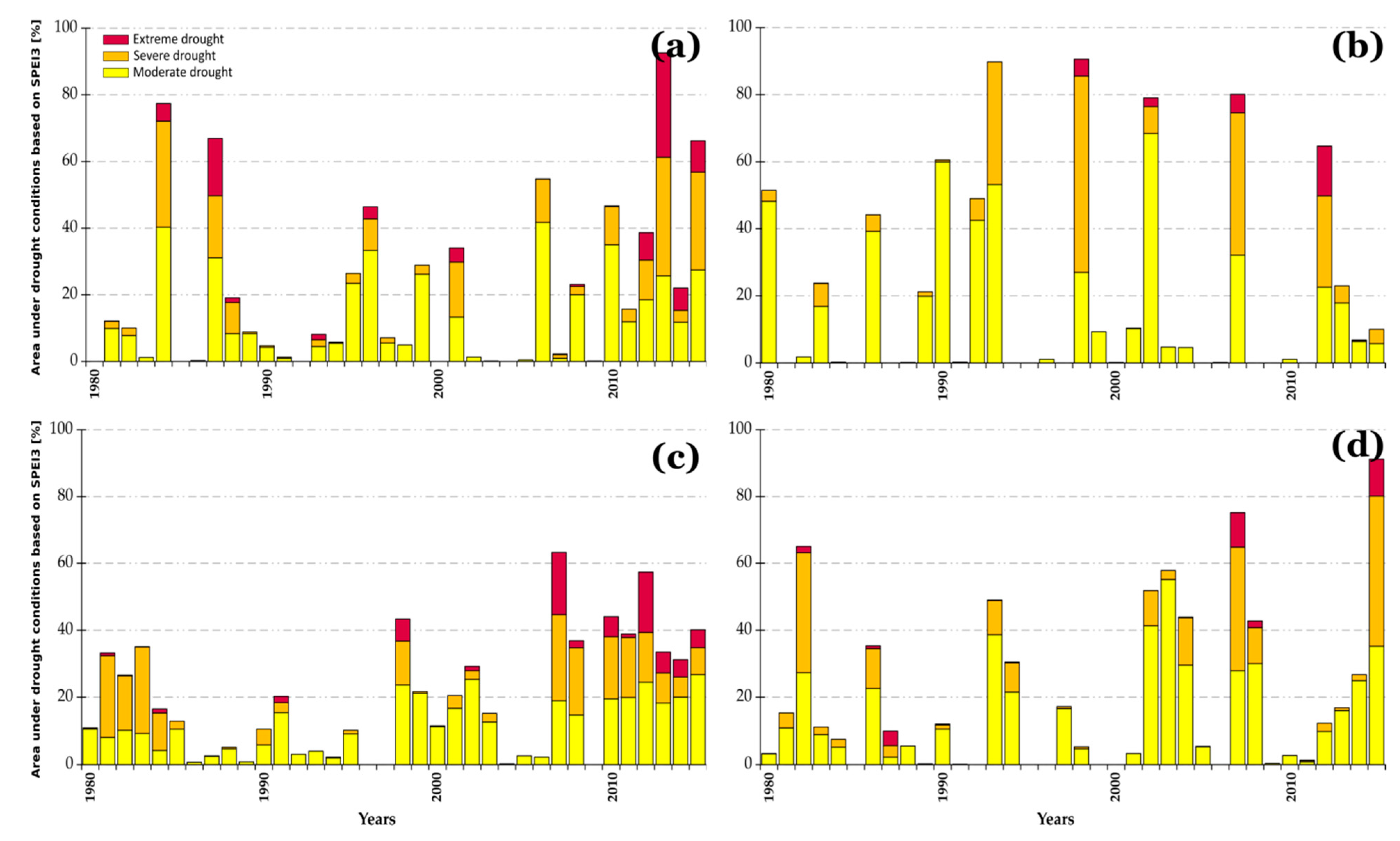
3.2. Temporal Variations of the Area under Drought Condition Based on SPEI12 and SPEI3

The percentage of the area under drought conditions relative to the total area over SFRB for each SPEI12 drought category (see Table 2) was used to investigate whether there was an expansion of areas impacted by drought at an interannual scale during 1980–2015. From Figure 5, one can see that all SPEI12-December drought categories have different magnitudes of trend in terms of Theil–Sen’s slope, ranging from 0.001% to 0.015%. Those categorized as moderate drought showed the greatest magnitude of slope. However, neither of them was found to be significant (α = 0.05).

In order to have a more complete picture of the area under drought conditions in the SFRB, the SPEI3 drought categories for each season were analyzed (Figure 6). All SPEI3 drought categories showed a positive Theil–Sen’s slope, which indicates the increasing of the area under drought conditions. However, only those classified as moderate drought or extreme drought exhibited a significant monotonic trend (Theil–Sen’s slope: 0.379% and 0.01% with α = 0.05 for moderate and extreme droughts) into the winter season (i.e., JJA) since the 1980s.

The winter months correspond to the dry season in the SFRB. Thus, these findings indicate an intensification of drought conditions in the basin, with a dry season becoming drier and geographically more extensive (see Figure 4c and Figure 6c). The next section further explores the incidence of extreme drought events which are characterized by an area under drought conditions greater than 40% for at least five consecutive months.

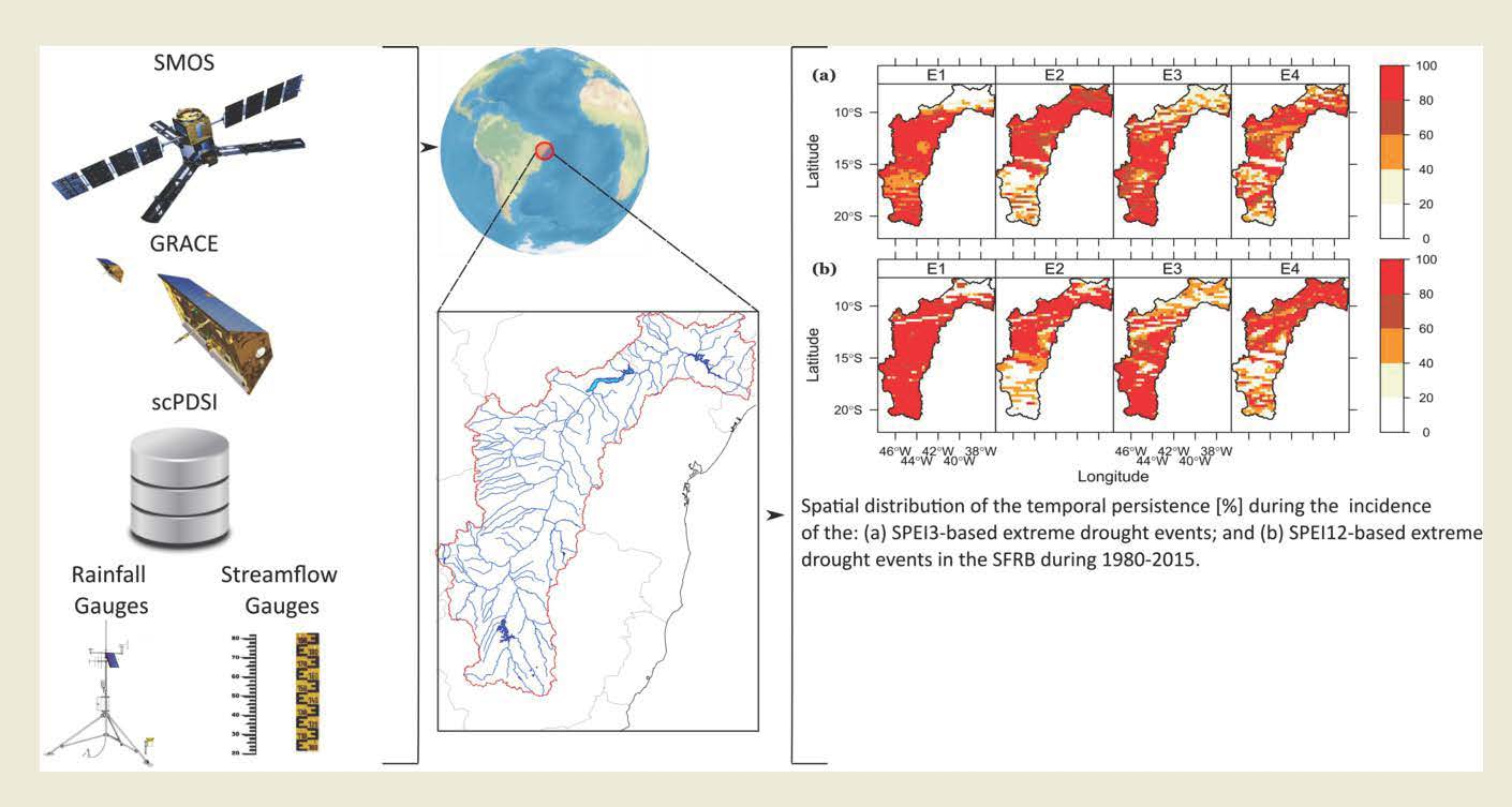
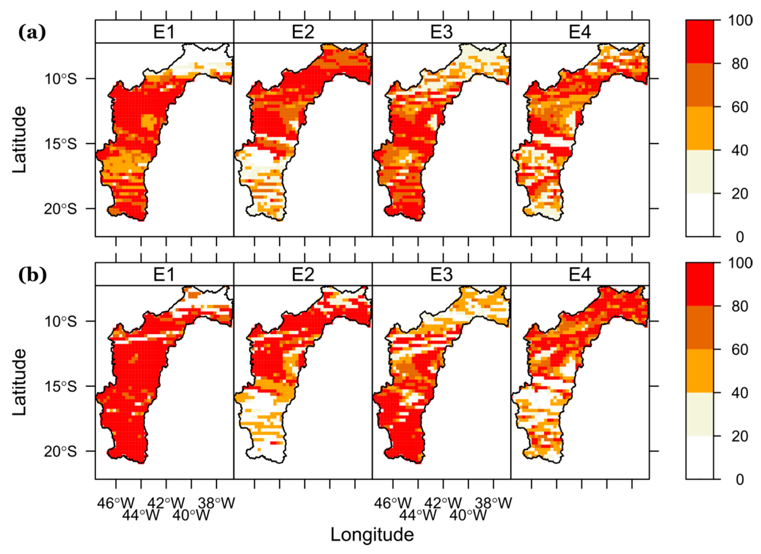
3.3. Extreme Drought Events for the Period 1980–2015

Table 3. Main features of the extreme drought events identified over the SFRB during 1980–2015.

Time Scale [Months]	Event	Start [Date]	End [Date]	Duration [Months]	Average SPEI [-] 1	Dry Area Peak [%] 2	Severity [-]
SPEI3	E1	April-98	October-98	7	−1.69	90.58	11.82
	E2	May-07	January-08	9	−1.73	80.09	15.61
	E3	March-12	October-12	8	−1.78	94.67	14.27
	E4	August-15	December-15	5	−1.75	95.99	8.76
SPEI12	E1	April-98	November-98	8	−1.76	90.69	14.06
	E2	October-07	August-08	11	−1.73	87.16	19.00
	E3	April-12	November-13	20	−1.83	92.93	36.55
	E4	January-14	December-15	21	−1.86	91.86	44.63

For the extreme drought event shown: ¹ it was calculated considering only values of SPEI ≤ −1.00; ² it is the maximum value of the percentage of pixels with values of SPEI ≤ −1.00. The values in bold correspond to the extreme value for each time scale and feature.

shows the main characteristics of the extreme drought events in the SFRB during 1980−2015. As has already been mentioned, the severity is defined as the absolute value of the sum of the values of the SPEI from the start to end of the dry spell. The most severe event for each time scale occurred from May 2007 to January 2008 (SPEI3) and from January 2014 to December 2015 (SPEI12). This last event was the worst extreme drought event in terms of severity (44.63), duration (21 months), and spatial coverage (91.86%). From Table 3, it can also be seen that the temporal distribution of the severity and duration of the SPEI3-based extreme drought events is approximately bell-shaped, with a peak during the occurrence of the E2 event. According to this result, there was no clear evidence of trends in the observed severity and duration for this type of event. On the other hand, the severity of the SPEI12-based events tended to increase between 1980 and 2015, which is consistent with the long-term drying trend observed over a large part of the SFRB (see Figure 3) and agrees with previous studies [11,29,45].

To explore the extreme drought events in terms of their temporal persistence, each of them was isolated. Then, the temporal persistence was calculated for each pixel using the procedure described in Section 2.3. Figure 7 shows the spatial distribution of the temporal persistence over the SFRB during the incidence of the SPEI3 and SPEI12 extreme drought events. For a given pixel, the value 100% means that the drought conditions prevailed throughout the entire duration. When this particular situation was assessed for each time scale, the results revealed that it occurred in a relatively constant proportion of the SFRB during the incidence of the SPEI3 extreme drought events (from 30% to 34% of the SFRB) compared to that caused by the SPEI12 extreme drought events (from 8% to 48% of the SFRB). Although the northern SFRB is located in the NEB, the areas with the highest temporal persistence of drought conditions tended to be slightly more frequent in the upper and middle parts of the basin. This outcome is in line with the findings reported in recent studies that found higher incidence of dry spells over that region than at the lower portion of the SFRB [11,29]. This fact has been mainly attributed to large-scale oceanic-climatic drivers and their interactions [10], such as ENSO [12], the Madden Julian Oscillation (MJO [14]), Pacific Decadal Oscillation (PDO [93]), and Atlantic Multidecadal Oscillation (AMO [94]).

Naturally, meteorological drought has a strong association with the soil moisture, streamflow, and groundwater variations. Therefore, different agricultural and hydrological drought indices have been used to assess their impacts on these components of the basin-scale hydrologic cycle [17,22,95]. The next two sections present a detailed examination of the land–atmosphere coupling during the drought events in the SFRB.

3.4. Paired Intercomparison between the Drought Indices

Unlike in Section 3.1 and Section 3.2, detrended full time series of all drought indices have been used in this and the following section. The Spearman correlation coefficient (R) for the SPEI3 against the SWDISa (R value: 0.665) and scPDSI (R value: 0.680), and for the SPEI12 against the WSDI (R value: 0.772) and scPDSI (R value: 0.700) showed the highest magnitudes (

Table 4. Spearman rank correlation coefficients between the SPEI3 and SPEI12 and the SWDISa, scPDSI, SSI, WSDI, and GGDI in the SFRB during their common time periods ¹.

Type of Drought	Drought Index	Site	Common Time Period	SPEI3 [-]	SPEI12 [-]
Agricultural	SWDISa [-]	-	Jun 2010 to December 2015	0.665 *	0.388 *
	scPDSI [-]	-	Jan 1981 to December 2015	0.680 *	0.700 *
Hydrological	SSI3	Propriá	Mar/Dec 1980 to December 2015	0.028	0.362 *
	SSI12	Propriá	Dec 1980 to December 2015	−0.026	0.221 *
	WSDI	-	Apr 2002 to December 2015	0.555 *	0.772 *
	GGDI	-	May 2002 to December 2015	−0.036	−0.007

¹ For each drought index, the Spearman correlation coefficient with the highest magnitude is reported in bold; * statistical significance at 95% level based on an asymptotic t approximation.

). Note that the SWDISa and scPDSI are more sensitive than other drought indices to short-term changes in precipitation reflected by the SPEI3. This was an expected result, since during the short-term droughts, the surface and root-zone SM are largely controlled by evaporation losses [24].

Strikingly, the corresponding values of Spearman R for the SPEI12-WSDI (R value: 0.772) and SPEI12-scPDSI (R value: 0.700) were similar to those for SPEI3. Figure 1b and Figure 8 help to explain this apparent inconsistency. The discharge of the São Francisco River at Propriá and other sites located downstream is profoundly affected in terms of magnitude and temporal regime by the operational management of the major reservoirs situated in the upper and middle parts of the SFRB (e.g., Três Marias, Sobradinho, and Itaparica; see Figure 1b). This situation, in turn, delays the propagation process of meteorological drought to hydrological drought [20] (see Figure 8). This feature also explains the weak correlation between the SPEI and SSI, particularly on a short-term time scale. Therefore, these correlations should be considered as spurious correlations that lack a causal basis. The reservoirs are filled during the rainy season and then during the dry season the stored water volume is progressively drained to approximately half its capacity [45], masking the climate signal triggered by droughts. Regarding the weak correlation between SPEI and GDDI, this can be attributed to the effect of aquifers in the SFRB. These results agree with the well-known fact that these aquifers respond very slowly to drought conditions [96].

As expected, the SPEI12-based extreme drought events E2, E3, and E4 were concomitant with downward trends in the soil moisture (Figure 8b,c), streamflow (Figure 8e,f), and total water storage (Figure 8g). Furthermore, the GGDI showed a moderate negative correlation with the SWDISa (Spearman R: −0.491) during 2010–2015, suggesting that there was an increase in groundwater abstractions which is in line with the expansion of irrigated agriculture in the basin [50]. A more detailed comparison of Figure 8b,h reveals that the GGDI and SWDISa had different degrees of temporal coherence in the time domain. However, this was most evident during the E4 event which was the worst long-term drought in terms of severity (see Table 3). A better understanding of coupling between different abovementioned drought indices can help to explain land–atmosphere interactions during the drought episodes in the SFRB. This has been the main motivation for using a wavelet squared coherence (WSC) analysis in next section.

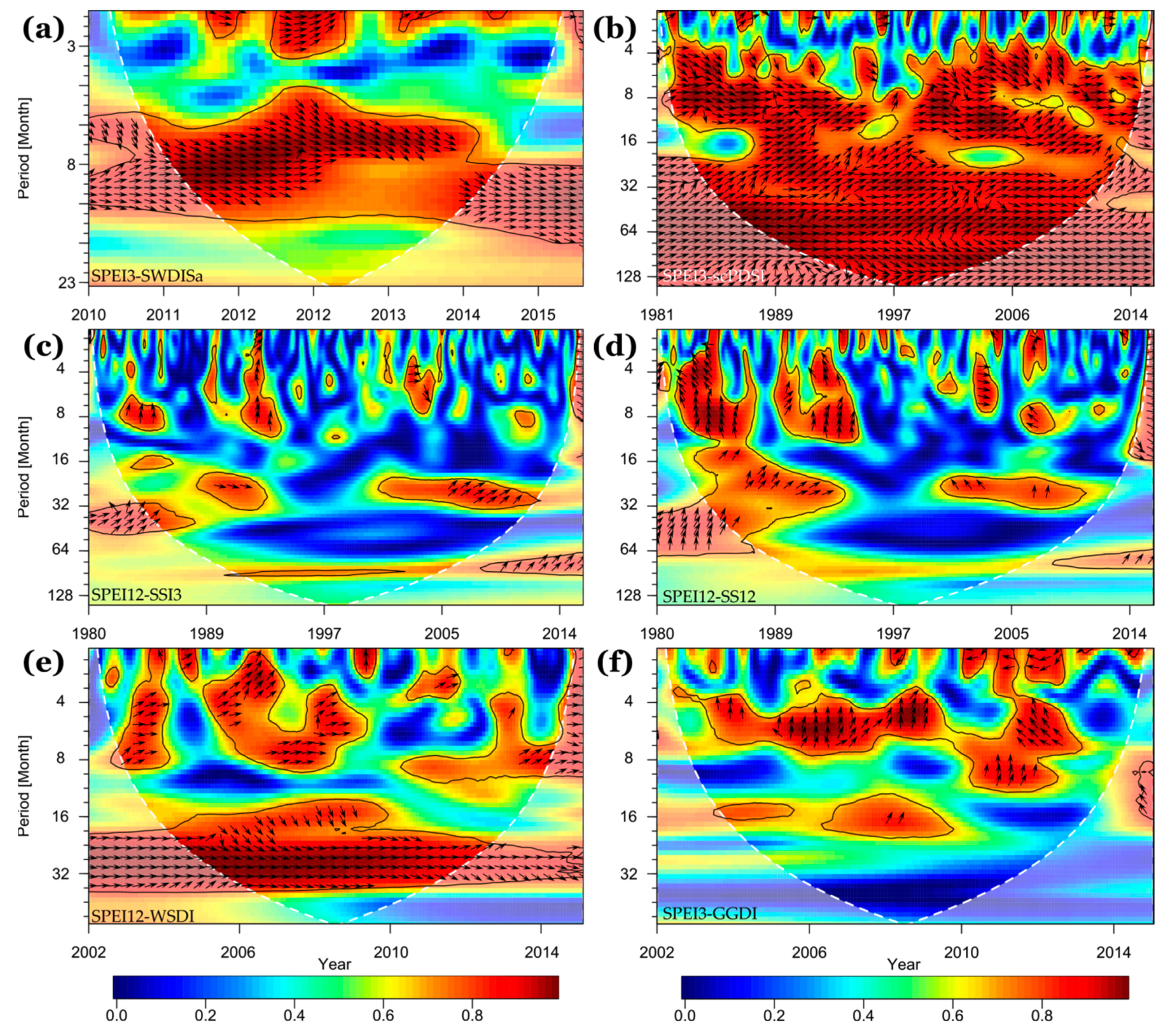
3.5. Coupling between the Drought Indices

Figure 9 displays the squared wavelet coherence together with their phases for SPEI3 and SPEI12 paired with those drought indices that showed the highest values of Spearman rank correlation coefficients in Table 4. The blue color indicates low wavelet coherence (near zero), whereas the red color shows areas of high wavelet coherence (near one).

The wavelet coherence between the SPEI3 and SWDISa revealed areas with the highest common power at recurrence intervals of 8–12 months from 2010 to 2015 (significant at 95% level). In this region, the signals of SPEI3 and SWDISa tended to be in phase (Figure 9a), indicating that there was a synchronous coupling at an interannual time scale. It should, however, be noted that the SPEI6/SPEI12-based E3 extreme drought events (see Table 3; from March 2012 to October 2012, and from April 2012 to November 2013, respectively), coincided with a strong relationship between both signals with recurrence times of 1–3 months. This means that, due to lack of precipitation and high temperature, the SSM in the SFRB was drastically affected in a very short period. Similarly, the scPDSI showed a synchronous and persistent coupling with the SPEI3 during the entire study period 1981–2015 (Figure 9b).

The SPEI12-SSI3 and SPEI12-SSI12 exhibited an asynchronous coupling in intensity and direction of the correlation during 1980–2015 (Figure 8c,d and Figure 9c,d). The SSI3 and SSI12 signals tended to lead the SPEI12 signal at recurrence intervals of 4–12 months (significant at 95% level). Obviously, the presence of a large number of reservoirs in the SFRB favored a better correspondence between these signals during the presence of extreme drought events and recurrence intervals greater than one year, which is congruent with the results in Figure 8.

Regarding the SPEI12-WSDI, they tended to show a strong coupling (significant at 95% level) in both short-term (i.e., 8–12 months) and long-term (i.e., ≥12 months) drought conditions (Figure 8e and Figure 9e), which was also reflected by the highest linear association shown in Table 4. This result highlights the effect of drought on water resources in the SFRB.

The SPEI3-GGDI revealed clear evidence of non-linearity between them (Figure 8e and Figure 9f). The areas with the highest common power were mainly concentrated at recurrence intervals less than a year. The GGDI signal tended to lead the SPEI3 signal, which is concurrent with the seasonal use of water for irrigation in the SFRB [49]. Nevertheless, it is important to mention that the signals of SPEI3 and GGDI tended to be in anti-phase from 2012 to 2015, implying that the drought conditions at interannual time scale increased groundwater abstraction, which, in turn, reduced groundwater storage.

Overall, these results indicate that the SWDISa and scPDSI capture reasonably well the short-term drought conditions. The WSDI represent adequately the hydrological droughts in terms of total water resources, while the GGDI has an acceptable performance in capturing the groundwater abstractions. In relation to the SSI3 and SSI12 at the streamflow gauge Propriá, due to the large number of reservoirs in the SFRB, they should not be used for decision making.

Among the drought indices evaluated, the scPDSI and WSDI have the advantage of providing updated information until 2020 (see Table 1) and both show the highest correlation with SPEI3 and SPEI12 in both frequency and time domains (Figure 9b,e), respectively. Thus, they were used in order to explore the more recent evolution of the agricultural and hydrological droughts in the SFRB. The more relevant results are presented in the following section.

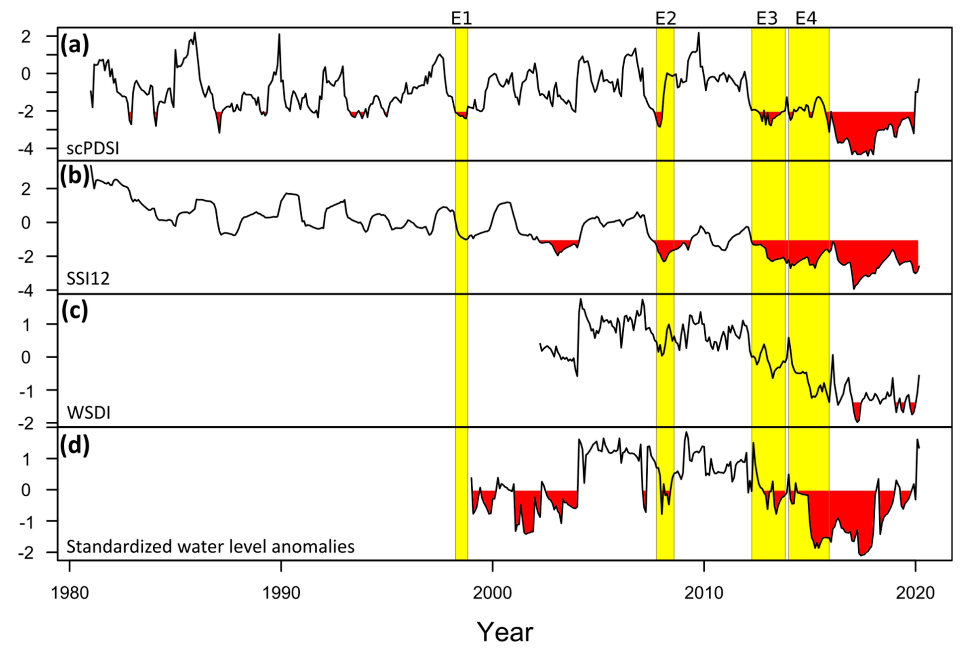
3.6. Recent Variations in Agriculture and Hydrological Drougths Based on scPDSI and WSDI

For this analysis, the water level of the Sobradinho reservoir and the discharge at the Boqueirão streamflow gauge (see Figure 1) were used as benchmark time series to infer the drought conditions in the upper and middle parts of the basin. Unlike the Propriá streamflow gauge, the tributary sub-basins to Boqueirão (about 69,995 km²) do not have relevant hydraulic and diversion structures, so the SSI12 time series can provide reliable information on hydrological drought conditions over this region of the basin. On the other hand, Sobradinho is the largest reservoir of the SFRB and is located in the lower part of the basin; hence, its depletion in terms of water level is a reasonable proxy of long-term drought impact in the upper and middle parts of the SFRB. Figure 10 summarizes the temporal variation of these variables. As noted by Sun et al. [11], and congruent with previous results, this basin experienced an overall soil moisture and water resources depletion situation since the beginning of 2012, coinciding with the occurrence of the SPEI12-based E3 and E4 extreme drought events.

An aspect relevant in Figure 10b is the presence of a moderate tendency towards drier-than-normal conditions over the Grande River basin, which drains into the Sao Francisco River near Boqueirão. This confirms the predominance of drought conditions in the western middle part of the SFRB shown in Figure 3 and Figure 4, persisting beyond the end of the 2020. Another key aspect observed in Figure 10 was an evident bounce-back effect in the scPDSI time series (January 2018), which may be attributed to the irrigation expansion policy throughout the SFRB [50]. Interestingly, the water level at the Sobradinho reservoir since 2019 showed a partial recovery from the 2012 and 2015 extreme drought events (Figure 10d) concurrent with the basin-scale WSDI (Spearman R: 0.760). This might be interpreted as an incipient signal of generalized recovery in the SFRB. However, this needs further investigation as it goes beyond the goal of this study.

4. Discussion

In this study, the concomitant impacts between the different types of droughts were analyzed in order to obtain a better understanding of their main features in the SFRB. The results revealed that a moderate basin-wide drying trend affected large parts of the middle and south regions of the SFRB from 1980 to 2015 (see Figure 3), where its main tributaries and reservoirs are located (see Figure 1a). The basin-scale drying was previously evidenced by Sun et al. [11], who identified an overall water depletion concomitant with a prolonged rainfall reduction, which in turn coincided with high SST anomalies over the Tropical North Atlantic (TNA) and strong El Niño episodes [10,12,97]. Although the degree of drying varied spatially, the severity of the drought increased during the JJA season and, to a lesser degree, in DJF and SON, respectively (see Figure 4). According to the assessment carried out by the Intergovernmental Panel for Climate Change (IPCC) in its Sixth Assessment Report, these variations are ascribed to the effects of climate change in this region of Brazil [98]. This carries significant implications for the agriculture and hydropower sectors [45,50] due to their high dependence on seasonal rainfall [8].

Regarding the performance of satellite-based drought indices in the characterization of droughts, the results revealed that the SWDISa and WSDI have the greatest potential for assessing and monitoring agricultural and hydrological droughts across the basin (see Figure 8). For the SWDISa case, this strength is due to the SMOS capacity to detect small variations in soil moisture at the top soil [7,97], whereas that the good performance of WSDI may be attributed to the capacity of the GRACE satellites to integrate terrestrial water storage vertically [42]. These satellite-based drought indices are periodically updated and upgraded as the GRACE and SMOS record lengths grow. This implies that they can provide complementary information on regional drought conditions which is useful to decision and policy makers in the SFRB.

Both satellite-based and ground-based drought indices used in this study revealed that there was no clear evidence of a trend in the short-term extreme drought events in terms of their spatial coverage, severity, or duration during 1980–2015. In contrast, the long-term extreme drought events tended to be spatially more extensive and temporally persistent (see Table 3 and Figure 7), which is consistent with the conclusions of previous studies [10,11]. Nevertheless, this finding is not necessarily indicative of an irreversible transition to drier-than-normal conditions in the basin. The concurrence of different climate modes of natural variability may explain part of the intensification of drought conditions in recent decades, as suggested by Kayano et al. [97]. They may act in synergy blocking the moisture transport from different oceanic regions to the basin, triggering strong drought conditions [99,100]. This statement is confirmed by several studies that found that the extreme drought events during the austral rainy season have been consistent with near surface atmospheric circulation changes and a reduced moisture flow coming from the tropical Atlantic region [10,12,18]. However, as a consequence of climate change, this synergistic effect is becoming more frequent after the 2000s (see Figure 10), leading to unprecedented drought events in the SFRB [4,101]. In this context, it is important to mention that the social, economic, and environmental impacts of drought are aggravated by anthropogenic factors such as the expansion of the irrigated agriculture and the building of small dams and other hydraulic infrastructures for human consumption and irrigation, which in turn pushes water demand [50]. In spite of this pessimistic situation, the agricultural expansion might be limited by the recurrent droughts (see Figure 8) in the short term. This is particularly relevant for crops with high water use demand such as rice and sugarcane.

The southern half of the SFRB already experiences high socioeconomic vulnerability and precarious conditions to face the impacts resulting from extreme droughts [8]. Nevertheless, the intensification on drought occurrence over the upper and middle regions of the SFRB (see Figure 5 and Figure 6) is of particular concern because the agricultural production is heavily based on rainfed crops in most of their municipalities [50]. On the other hand, the hydropower sector is not excluded from this reality. The hydropower generation in this region has shown a low resilience and adaptive capacity to strong drought conditions that continued until 2020 (see Figure 10d), resulting in blackouts, water supply restrictions, and energy shortages [102].

Another key aspect observed in our results was a marked depletion of groundwater levels (see Figure 8h) during the severe drought conditions, which was inversely proportional to the surface soil moisture content (see Figure 8b), implying an increase in groundwater abstraction for irrigation. This is not a good sign for the SFRB. An over-abstraction of groundwater stock during the occurrence of the prolonged extreme droughts can lead to irreversible depletion, particularly in the shallow aquifers [103].

The reduction of water availability due to recurrent drought events together with the expansion of irrigated agriculture and the increasing demand for hydraulic energy could increase the number of water use conflicts in the SFRB. Furthermore, an increased risk of food insecurity, environmental degradation among other potential impacts related to extreme drought episodes, would be expected in future. Last, but not least, this scenario leaves doubts about the long-term sustainability of the São Francisco River Integration Project conducted by the Brazilian federal government. However, according to the most recent data from the SWDISa and WSDI, prolonged drought conditions appear to be reversing (Figure 10a,c). In any case, the design and implementation of effective adaptation strategies will be necessary in the face of future droughts in the SFRB.

5. Conclusions

Several satellite-based and ground-based drought indices were used to better understand how climate variability is affecting the spatiotemporal distribution of extreme droughts in the SFRB. The newest version of the GRACE-based terrestrial water storage anomalies and SMOS-based soil moisture together with the scPDSI were used as satellite-based drought indices during different periods between 1981 and 2020. The SPEI and SSI at different time scales were used as ground-based drought indices and as benchmark data against which to assess the performance of the satellite-based drought indices in capturing drought conditions. This set of drought indices provided a comprehensive picture of drought risk in the basin. The following conclusions can be drawn from this study.

• A moderate basin-wide drying trend at annual time scale affected the middle and south regions of the SFRB from 1980 to 2015, coinciding with the ENSO phenomenon and SST anomalies in the tropical Atlantic, as already mentioned in previous studies.
• An expansion of the area under drought conditions was observed during the winter months (i.e., JJA), but there was no evidence of a significant positive trend in the remaining seasons in terms of spatial coverage between 1980 and 2015.
• The long-term extreme drought events showed increasing trends in terms of severity and duration, but this characteristic was not observed on a seasonal time scale during 1980–2015.
• The SWDISa and WSDI showed a good performance in assessing agricultural and hydrological droughts across the whole SFRB.
• A marked depletion of groundwater levels concurrent with increase in soil moisture content was observed during the most severe drought conditions, which means an intensification of the groundwater abstraction for irrigation.
• According to the most recent data from the SWDISa and WSDI, prolonged drought conditions appear to be reversing.

Overall, this paper has shown that drought conditions were worsening over the SFRB in terms of spatial coverage, duration, and severity during 1980–2015, which was particularly evident on longer time scales. Although it is too early to indicate a general decline in basin-scale drought conditions, the time series of water level at the Sobradinho reservoir shows incipient signs of a reversion of drought conditions since the end of 2019 (see Figure 10d). Consequently, this aspect will be explored as further information becomes available to improve our knowledge about how climate variability is affecting the distribution of extreme droughts in the SFRB.

References

1. Bakker, K. Water Security: Research Challenges and Opportunities. Science 2012, 337, 914–915. [Google Scholar] [CrossRef] [PubMed]
2. de Assis Souza Filho, F.; Formiga-Johnsson, R.M.; de Carvalho Studart, T.M.; Abicalil, M.T. From Drought to Water Security: Brazilian Experiences and Challenges. In Global Water Security; Springer: Berlin/Heidelberg, Germany, 2018; pp. 233–265. [Google Scholar]
3. Awange, J.L.; Mpelasoka, F.; Goncalves, R.M. When every drop counts: Analysis of Droughts in Brazil for the 1901–2013 period. Sci. Total Environ. 2016, 566–567, 1472–1488. [Google Scholar] [CrossRef] [PubMed] [Green Version]
4. Marengo, J.A.; Torres, R.R.; Alves, L.M. Drought in Northeast Brazil—Past, present, and future. Theor. Appl. Climatol. 2017, 129, 1189–1200. [Google Scholar] [CrossRef]
5. Marengo, J.A.; Chou, S.C.; Kay, G.; Alves, L.M.; Pesquero, J.F.; Soares, W.R.; Santos, D.C.; Lyra, A.A.; Sueiro, G.; Betts, R.; et al. Development of regional future climate change scenarios in South America using the Eta CPTEC/HadCM3 climate change projections: Climatology and regional analyses for the Amazon, São Francisco and the Paraná River basins. Clim. Dyn. 2012, 38, 1829–1848. [Google Scholar] [CrossRef]
6. Maneta, M.P.; Torres, M.; Wallender, W.W.; Vosti, S.; Kirby, M.; Bassoi, L.H.; Rodrigues, L.N. Water demand and flows in the São Francisco River Basin (Brazil) with increased irrigation. Agric. Water Manag. 2009, 96, 1191–1200. [Google Scholar] [CrossRef] [Green Version]
7. Paredes-Trejo, F.; Barbosa, H. Evaluation of the SMOS-Derived Soil Water Deficit Index as Agricultural Drought Index in Northeast of Brazil. Water 2017, 9, 377. [Google Scholar] [CrossRef]
8. Buriti, C.; Barbosa, H.A.; Paredes-Trejo, F.J.; Kumar, T.V.L.; Thakur, M.K.; Rao, K.K. Un Siglo de Sequías: ¿Por qué las Políticas de Agua no Desarrollaron la Región Semiárida Brasileña? Rev. Bras. Meteorol. 2020, 35, 683–688. [Google Scholar] [CrossRef]
9. Oliveira, D.H.M.C.; Lima, K.C.; Spyrides, M.H.C. Rainfall and streamflow extreme events in the São Francisco hydrographic region. Int. J. Climatol. 2021, 41, 1279–1291. [Google Scholar] [CrossRef]
10. Paredes Trejo, F.; Brito-Castillo, L.; Barbosa Alves, H.; Guevara, E. Main features of large-scale oceanic-atmospheric circulation related to strongest droughts during rainy season in Brazilian São Francisco River Basin. Int. J. Climatol. 2016, 36, 4102–4117. [Google Scholar] [CrossRef]
11. Sun, T.; Ferreira, V.; He, X.; Andam-Akorful, S. Water Availability of São Francisco River Basin Based on a Space-Borne Geodetic Sensor. Water 2016, 8, 213. [Google Scholar] [CrossRef]
12. Jimenez, J.C.; Marengo, J.A.; Alves, L.M.; Sulca, J.C.; Takahashi, K.; Ferrett, S.; Collins, M. The role of ENSO flavours and TNA on recent droughts over Amazon forests and the Northeast Brazil region. Int. J. Climatol. 2019, 41, 3761–3780. [Google Scholar] [CrossRef]
13. Santos, M.S.; Costa, V.A.F.; dos Santos Fernandes, W.; de Paes, R.P. Time-space characterization of droughts in the São Francisco river catchment using the Standard Precipitation Index and continuous wavelet transform. Rev. Bras. Recur. Hidricos 2019, 24, 1–12. [Google Scholar] [CrossRef] [Green Version]
14. Giovannettone, J.; Paredes-Trejo, F.; Barbosa, H.; Santos, C.A.C.; Kumar, T.V.L. Characterization of links between hydro-climate indices and long-term precipitation in Brazil using correlation analysis. Int. J. Climatol. 2020, 40, 5527–5541. [Google Scholar] [CrossRef]
15. Stolf, R.; de S Piedade, S.M.; da Silva, J.R.; da Silva, L.C.F.; Maniero, M.Â. Water transfer from São Francisco river to semiarid northeast of Brazil: Technical data, environmental impacts, survey of opinion about the amount to be transferred. Eng. Agrícola 2012, 32, 998–1010. [Google Scholar] [CrossRef] [Green Version]
16. Guimarães, J.A., Jr. Reforma hidrica do Nordeste como alternativa à transposição do rio São Francisco. Cad. CEAS Rev. Crítica Humanid. 2016, 80–88. Available online: https://cadernosdoceas.ucsal.br/index.php/cadernosdoceas/article/view/135 (accessed on 15 January 2021).
17. Mishra, A.K.; Singh, V.P. A review of drought concepts. J. Hydrol. 2010, 391, 202–216. [Google Scholar] [CrossRef]
18. Cunha, A.P.M.A.; Zeri, M.; Deusdará Leal, K.; Costa, L.; Cuartas, L.A.; Marengo, J.A.; Tomasella, J.; Vieira, R.M.; Barbosa, A.A.; Cunningham, C.; et al. Extreme Drought Events over Brazil from 2011 to 2019. Atmosphere 2019, 10, 642. [Google Scholar] [CrossRef] [Green Version]
19. Cunha, A.P.M.; Alvalá, R.C.; Nobre, C.A.; Carvalho, M.A. Monitoring vegetative drought dynamics in the Brazilian semiarid region. Agric. For. Meteorol. 2015, 214–215, 494–505. [Google Scholar] [CrossRef]
20. Van Loon, A.F.; Laaha, G. Hydrological drought severity explained by climate and catchment characteristics. J. Hydrol. 2015, 526, 3–14. [Google Scholar] [CrossRef] [Green Version]
21. Mehran, A.; Mazdiyasni, O.; AghaKouchak, A. A hybrid framework for assessing socioeconomic drought: Linking climate variability, local resilience, and demand. J. Geophys. Res. Atmos. 2015, 120, 7520–7533. [Google Scholar] [CrossRef]
22. Zargar, A.; Sadiq, R.; Naser, B.; Khan, F.I. A review of drought indices. Environ. Rev. 2011, 19, 333–349. [Google Scholar] [CrossRef]
23. Sheffield, J.; Wood, E.F. Drought; Earthscan: London, UK, 2012; ISBN 9781849775250. [Google Scholar]
24. Park, S.-Y.; Sur, C.; Kim, J.-S.; Lee, J.-H. Evaluation of multi-sensor satellite data for monitoring different drought impacts. Stoch. Environ. Res. Risk Assess. 2018, 32, 2551–2563. [Google Scholar] [CrossRef]
25. Sur, C.; Hur, J.; Kim, K.; Choi, W.; Choi, M. An evaluation of satellite-based drought indices on a regional scale. Int. J. Remote Sens. 2015, 36, 5593–5612. [Google Scholar] [CrossRef]
26. Mu, Q.; Zhao, M.; Kimball, J.S.; McDowell, N.G.; Running, S.W. A Remotely Sensed Global Terrestrial Drought Severity Index. Bull. Am. Meteorol. Soc. 2013, 94, 83–98. [Google Scholar] [CrossRef] [Green Version]
27. Jafari, S.M.; Nikoo, M.R.; Dehghani, M.; Alijanian, M. Evaluation of two satellite-based products against ground-based observation for drought analysis in the southern part of Iran. Nat. Hazards 2020, 102, 1249–1267. [Google Scholar] [CrossRef]
28. Shahzaman, M.; Zhu, W.; Ullah, I.; Mustafa, F.; Bilal, M.; Ishfaq, S.; Nisar, S.; Arshad, M.; Iqbal, R.; Aslam, R.W. Comparison of Multi-Year Reanalysis, Models, and Satellite Remote Sensing Products for Agricultural Drought Monitoring over South Asian Countries. Remote Sens. 2021, 13, 3294. [Google Scholar] [CrossRef]
29. Santos, C.A.G.; Brasil Neto, R.M.; Passos, J.S.d.A.; da Silva, R.M. Drought assessment using a TRMM-derived standardized precipitation index for the upper São Francisco River basin, Brazil. Environ. Monit. Assess. 2017, 189, 250. [Google Scholar] [CrossRef] [PubMed]
30. Vicente-Serrano, S.M.; Beguería, S.; López-Moreno, J.I. A Multiscalar Drought Index Sensitive to Global Warming: The Standardized Precipitation Evapotranspiration Index. J. Clim. 2010, 23, 1696–1718. [Google Scholar] [CrossRef] [Green Version]
31. Martínez-Fernández, J.; González-Zamora, A.; Sánchez, N.; Gumuzzio, A.; Herrero-Jiménez, C.M. Satellite soil moisture for agricultural drought monitoring: Assessment of the SMOS derived Soil Water Deficit Index. Remote Sens. Environ. 2016, 177, 277–286. [Google Scholar] [CrossRef]
32. Wells, N.; Goddard, S.; Hayes, M.J. A Self-Calibrating Palmer Drought Severity Index. J. Clim. 2004, 17, 2335–2351. [Google Scholar] [CrossRef]
33. Vicente-Serrano, S.M.; López-Moreno, J.I.; Begueria, S.; Lorenzo-Lacruz, J.; Azorin-Molina, C.; Morán-Tejeda, E. Accurate computation of a streamflow drought index. J. Hydrol. Eng. 2012, 17, 318–332. [Google Scholar] [CrossRef] [Green Version]
34. Thomas, A.C.; Reager, J.T.; Famiglietti, J.S.; Rodell, M. A GRACE-based water storage deficit approach for hydrological drought characterization. Geophys. Res. Lett. 2014, 41, 1537–1545. [Google Scholar] [CrossRef] [Green Version]
35. Thomas, B.F.; Famiglietti, J.S.; Landerer, F.W.; Wiese, D.N.; Molotch, N.P.; Argus, D.F. GRACE Groundwater Drought Index: Evaluation of California Central Valley groundwater drought. Remote Sens. Environ. 2017, 198, 384–392. [Google Scholar] [CrossRef]
36. Beguería, S.; Vicente-Serrano, S.M.; Reig, F.; Latorre, B. Standardized precipitation evapotranspiration index (SPEI) revisited: Parameter fitting, evapotranspiration models, tools, datasets and drought monitoring. Int. J. Climatol. 2014, 34, 3001–3023. [Google Scholar] [CrossRef] [Green Version]
37. Stagge, J.H.; Tallaksen, L.M.; Gudmundsson, L.; Van Loon, A.F.; Stahl, K. Candidate Distributions for Climatological Drought Indices (SPI and SPEI). Int. J. Climatol. 2015, 35, 4027–4040. [Google Scholar] [CrossRef]
38. Martinez-Fernández, J.; González-Zamora, A.; Sánchez, N.; Gumuzzio, A. A soil water based index as a suitable agricultural drought indicator. J. Hydrol. 2015, 522, 265–273. [Google Scholar] [CrossRef]
39. Scaini, A.; Sánchez, N.; Vicente-Serrano, S.M.; Martínez-Fernández, J. SMOS-derived soil moisture anomalies and drought indices: A comparative analysis using in situ measurements. Hydrol. Process. 2015, 29, 373–383. [Google Scholar] [CrossRef]
40. Modarres, R. Streamflow drought time series forecasting. Stoch. Environ. Res. Risk Assess. 2007, 21, 223–233. [Google Scholar] [CrossRef]
41. Telesca, L.; Lovallo, M.; Lopez-Moreno, I.; Vicente-Serrano, S. Investigation of scaling properties in monthly streamflow and Standardized Streamflow Index (SSI) time series in the Ebro basin (Spain). Phys. A Stat. Mech. Its Appl. 2012, 391, 1662–1678. [Google Scholar] [CrossRef]
42. Nigatu, Z.M.; Fan, D.; You, W.; Melesse, A.M. Hydroclimatic Extremes Evaluation Using GRACE/GRACE-FO and Multidecadal Climatic Variables over the Nile River Basin. Remote Sens. 2021, 13, 651. [Google Scholar] [CrossRef]
43. Almagro, A.; Oliveira, P.T.S.; Meira Neto, A.A.; Roy, T.; Troch, P. CABra: A novel large-sample dataset for Brazilian catchments. Hydrol. Earth Syst. Sci. Discuss. 2020, 2020, 1–40. [Google Scholar]
44. Torres, M.d.O.; Vosti, S.A.; Maneta, M.P.; Wallender, W.W.; Rodrigues, L.N.; Bassoi, L.H.; Young, J.A. Spatial patterns of rural poverty: An exploratory analysis in the São Francisco River Basin, Brazil. Nov. Econ. 2011, 21, 45–66. [Google Scholar] [CrossRef]
45. de Jong, P.; Tanajura, C.A.S.; Sánchez, A.S.; Dargaville, R.; Kiperstok, A.; Torres, E.A. Hydroelectric production from Brazil’s São Francisco River could cease due to climate change and inter-annual variability. Sci. Total Environ. 2018, 634, 1540–1553. [Google Scholar] [CrossRef] [PubMed]
46. Beck, H.E.; Zimmermann, N.E.; McVicar, T.R.; Vergopolan, N.; Berg, A.; Wood, E.F. Present and future Köppen-Geiger climate classification maps at 1-km resolution. Sci. Data 2018, 5, 180214. [Google Scholar] [CrossRef] [Green Version]
47. Braga, B.P.F.; Lotufo, J.G. Integrated River Basin Plan in Practice: The São Francisco River Basin. Int. J. Water Resour. Dev. 2008, 24, 37–60. [Google Scholar] [CrossRef]
48. Marengo, J.A.; Alves, L.M.; Alvala, R.C.; Cunha, A.P.; Brito, S.; Moraes, O.L.L. Climatic characteristics of the 2010–2016 drought in the semiarid Northeast Brazil region. An. Acad. Bras. Cienc. 2018, 90, 1973–1985. [Google Scholar] [CrossRef]
49. Liu, X.; Yu, L.; Si, Y.; Zhang, C.; Lu, H.; Yu, C.; Gong, P. Identifying patterns and hotspots of global land cover transitions using the ESA CCI Land Cover dataset. Remote Sens. Lett. 2018, 9, 972–981. [Google Scholar] [CrossRef]
50. Ferrarini, A.d.S.F.; Ferreira Filho, J.B.d.S.; Cuadra, S.V.; Victoria, D.d.C. Water demand prospects for irrigation in the São Francisco River: Brazilian public policy. Water Policy 2020, 22, 449–467. [Google Scholar] [CrossRef] [Green Version]
51. Berry, P.A.M.; Garlick, J.D.; Smith, R.G. Near-global validation of the SRTM DEM using satellite radar altimetry. Remote Sens. Environ. 2007, 106, 17–27. [Google Scholar] [CrossRef]
52. Xavier, A.C.; King, C.W.; Scanlon, B.R. Daily gridded meteorological variables in Brazil (1980–2013). Int. J. Climatol. 2016, 36, 2644–2659. [Google Scholar] [CrossRef] [Green Version]
53. Allen, R.G.; Pereira, L.S.; Raes, D.; Smith, M. Crop Evapotranspiration-Guidelines for Computing Crop Water Requirements; FAO Irrigation and Drainage Paper 56; FAO: Rome, Italy, 1998. [Google Scholar]
54. Xavier, A.C. An update of Xavier, King and Scanlon (2016) daily precipitation gridded data set for the Brazil. In Proceedings of the 18th Brazilian Symposium on Remote Sensing, Santos, São Paulo, Brazil, 28–31 May 2017; pp. 28–33. [Google Scholar]
55. Ryan, K.F.; Giles, D.E.A. Testing for Unit Roots with Missing Observations; Econometrics Working Papers 9802; University of Victoria: Victoria, BC, Canada, 1998. [Google Scholar]
56. Moritz, S.; Bartz-Beielstein, T. imputeTS: Time series missing value imputation in R. R J. 2017, 9, 207–218. [Google Scholar] [CrossRef] [Green Version]
57. Kerr, Y.H.; Al-Yaari, A.; Rodriguez-Fernandez, N.; Parrens, M.; Molero, B.; Leroux, D.; Bircher, S.; Mahmoodi, A.; Mialon, A.; Richaume, P.; et al. Overview of SMOS performance in terms of global soil moisture monitoring after six years in operation. Remote Sens. Environ. 2016, 180, 40–63. [Google Scholar] [CrossRef]
58. González-Zamora, Á.; Sánchez, N.; Martínez-Fernández, J.; Gumuzzio, Á.; Piles, M.; Olmedo, E. Long-term SMOS soil moisture products: A comprehensive evaluation across scales and methods in the Duero Basin (Spain). Phys. Chem. Earth Parts A/B/C 2015, 83–84, 123–136. [Google Scholar] [CrossRef]
59. Spatafora, L.R.; Vall-llossera, M.; Camps, A.; Chaparro, D.; Alvalá, R.C.d.S.; Barbosa, H. Validation of SMOS L3 AND L4 Soil Moisture Products In The Remedhus (SPAIN) AND CEMADEN (BRAZIL) Networks. Rev. Bras. Geogr. Física 2020, 13, 691. [Google Scholar] [CrossRef]
60. Kornfeld, R.P.; Arnold, B.W.; Gross, M.A.; Dahya, N.T.; Klipstein, W.M.; Gath, P.F.; Bettadpur, S. GRACE-FO: The Gravity Recovery and Climate Experiment Follow-On Mission. J. Spacecr. Rockets 2019, 56, 931–951. [Google Scholar] [CrossRef]
61. Tapley, B.D.; Bettadpur, S.; Watkins, M.; Reigber, C. The gravity recovery and climate experiment: Mission overview and early results. Geophys. Res. Lett. 2004, 31. [Google Scholar] [CrossRef] [Green Version]
62. Save, H.; Bettadpur, S.; Tapley, B.D. High-resolution CSR GRACE RL05 mascons. J. Geophys. Res. Solid Earth 2016, 121, 7547–7569. [Google Scholar] [CrossRef]
63. Boergens, E.; Dobslaw, H.; Dill, R.; Thomas, M.; Dahle, C.; Murböck, M.; Flechtner, F. Modelling spatial covariances for terrestrial water storage variations verified with synthetic GRACE-FO data. GEM—Int. J. Geomath. 2020, 11, 24. [Google Scholar] [CrossRef]
64. Watkins, M.M.; Wiese, D.N.; Yuan, D.-N.; Boening, C.; Landerer, F.W. Improved methods for observing Earth’s time variable mass distribution with GRACE using spherical cap mascons. J. Geophys. Res. Solid Earth 2015, 120, 2648–2671. [Google Scholar] [CrossRef]
65. Sakumura, C.; Bettadpur, S.; Bruinsma, S. Ensemble prediction and intercomparison analysis of GRACE time-variable gravity field models. Geophys. Res. Lett. 2014, 41, 1389–1397. [Google Scholar] [CrossRef]
66. Getirana, A. Extreme Water Deficit in Brazil Detected from Space. J. Hydrometeorol. 2016, 17, 591–599. [Google Scholar] [CrossRef]
67. Melo, D.C.D.; Xavier, A.C.; Bianchi, T.; Oliveira, P.T.S.; Scanlon, B.R.; Lucas, M.C.; Wendland, E. Performance evaluation of rainfall estimates by TRMM Multi-satellite Precipitation Analysis 3B42V6 and V7 over Brazil. J. Geophys. Res. Atmos. 2015, 120, 9426–9436. [Google Scholar] [CrossRef] [Green Version]
68. Gadelha, A.N.; Coelho, V.H.R.; Xavier, A.C.; Barbosa, L.R.; Melo, D.C.D.; Xuan, Y.; Huffman, G.J.; Petersen, W.A.; Almeida, C. das N. Grid box-level evaluation of IMERG over Brazil at various space and time scales. Atmos. Res. 2019, 218, 231–244. [Google Scholar] [CrossRef] [Green Version]
69. Lima, C.H.R.; AghaKouchak, A. Droughts in Amazonia: Spatiotemporal Variability, Teleconnections, and Seasonal Predictions. Water Resour. Res. 2017, 53, 10824–10840. [Google Scholar] [CrossRef] [Green Version]
70. Bai, X.; Shen, W.; Wu, X.; Wang, P. Applicability of long-term satellite-based precipitation products for drought indices considering global warming. J. Environ. Manag. 2020, 255, 109846. [Google Scholar] [CrossRef]
71. Junqueira, R.; Viola, M.R.; de Mello, C.R.; Vieira-Filho, M.; Alves, M.V.G.; Amorim, J. da S. Drought severity indexes for the Tocantins River Basin, Brazil. Theor. Appl. Climatol. 2020, 141, 465–481. [Google Scholar] [CrossRef]
72. Tijdeman, E.; Stahl, K.; Tallaksen, L.M. Drought Characteristics Derived Based on the Standardized Streamflow Index: A Large Sample Comparison for Parametric and Nonparametric Methods. Water Resour. Res. 2020, 56, e2019WR026315. [Google Scholar] [CrossRef]
73. Hunt, E.D.; Hubbard, K.G.; Wilhite, D.A.; Arkebauer, T.J.; Dutcher, A.L. The development and evaluation of a soil moisture index. Int. J. Climatol. 2009, 29, 747–759. [Google Scholar] [CrossRef]
74. van der Schrier, G.; Barichivich, J.; Briffa, K.R.; Jones, P.D. A scPDSI-based global data set of dry and wet spells for 1901–2009. J. Geophys. Res. Atmos. 2013, 118, 4025–4048. [Google Scholar] [CrossRef]
75. Hu, K.; Awange, J.L.; Khandu; Forootan, E.; Goncalves, R.M.; Fleming, K. Hydrogeological characterisation of groundwater over Brazil using remotely sensed and model products. Sci. Total Environ. 2017, 599–600, 372–386. [Google Scholar] [CrossRef] [Green Version]
76. Wang, F.; Wang, Z.; Yang, H.; Di, D.; Zhao, Y.; Liang, Q. Utilizing GRACE-based groundwater drought index for drought characterization and teleconnection factors analysis in the North China Plain. J. Hydrol. 2020, 585, 124849. [Google Scholar] [CrossRef]
77. Rodell, M.; Houser, P.R.; Jambor, U.; Gottschalck, J.; Mitchell, K.; Meng, C.-J.; Arsenault, K.; Cosgrove, B.; Radakovich, J.; Bosilovich, M.; et al. The Global Land Data Assimilation System. Bull. Am. Meteorol. Soc. 2004, 85, 381–394. [Google Scholar] [CrossRef] [Green Version]
78. Abatzoglou, J.T.; Dobrowski, S.Z.; Parks, S.A.; Hegewisch, K.C. TerraClimate, a high-resolution global dataset of monthly climate and climatic water balance from 1958–2015. Sci. Data 2018, 5, 170191. [Google Scholar] [CrossRef] [PubMed] [Green Version]
79. Hu, Z.; Liu, S.; Zhong, G.; Lin, H.; Zhou, Z. Modified Mann-Kendall trend test for hydrological time series under the scaling hypothesis and its application. Hydrol. Sci. J. 2020, 65, 2419–2438. [Google Scholar] [CrossRef]
80. Yue, S.; Wang, C. The Mann-Kendall Test Modified by Effective Sample Size to Detect Trend in Serially Correlated Hydrological Series. Water Resour. Manag. 2004, 18, 201–218. [Google Scholar] [CrossRef]
81. Theil, H. A Rank-Invariant Method of Linear and Polynomial Regression Analysis. In Henri Theil’s Contributions to Economics and Econometrics; Springer: Berlin/Heidelberg, Germany, 1992; pp. 345–381. [Google Scholar]
82. McKee, T.B.; Doesken, N.J.; Kleist, J. The relationship of drought frequency and duration to time scales. In Proceedings of the 8th Conference on Applied Climatology, Anaheim, CA, USA, 17–22 January 1993; Volume 17, pp. 179–183. [Google Scholar]
83. Junqueira, R.; Viola, M.R.; Amorim, J.S.; Mello, C.R. Hydrological Response to Drought Occurrences in a Brazilian Savanna Basin. Resources 2020, 9, 123. [Google Scholar] [CrossRef]
84. Paredes-Trejo, F.; Barbosa, H.A.; Giovannettone, J.; Lakshmi Kumar, T.V.; Thakur, M.K.; de Oliveira Buriti, C. Long-Term Spatiotemporal Variation of Droughts in the Amazon River Basin. Water 2021, 13, 351. [Google Scholar] [CrossRef]
85. Podobnik, B.; Stanley, H.E. Detrended Cross-Correlation Analysis: A New Method for Analyzing Two Nonstationary Time Series. Phys. Rev. Lett. 2008, 100, 084102. [Google Scholar] [CrossRef] [Green Version]
86. Yue, S.; Pilon, P.; Cavadias, G. Power of the Mann–Kendall and Spearman’s rho tests for detecting monotonic trends in hydrological series. J. Hydrol. 2002, 259, 254–271. [Google Scholar] [CrossRef]
87. Wu, H.; Zou, Y.; Alves, L.M.; Macau, E.E.N.; Sampaio, G.; Marengo, J.A. Uncovering episodic influence of oceans on extreme drought events in Northeast Brazil by ordinal partition network approaches. Chaos Interdiscip. J. Nonlinear Sci. 2020, 30, 053104. [Google Scholar] [CrossRef]
88. Labat, D.; Ronchail, J.; Callede, J.; Guyot, J.L.; De Oliveira, E.; Guimarães, W. Wavelet analysis of Amazon hydrological regime variability. Geophys. Res. Lett. 2004, 31, 3–6. [Google Scholar] [CrossRef] [Green Version]
89. Torrence, C.; Compo, G.P. A Practical Guide to Wavelet Analysis. Bull. Am. Meteorol. Soc. 1998, 79, 61–78. [Google Scholar] [CrossRef] [Green Version]
90. Grinsted, A.; Moore, J.C.; Jevrejeva, S. Application of the cross wavelet transform and wavelet coherence to geophysical time series. Nonlinear Process. Geophys. 2004, 11, 561–566. [Google Scholar] [CrossRef]
91. Gouhier, T.C.; Grinsted, A.; Simko, V.; Gouhier, M.T.C.; Rcpp, L. R Package Biwavelet: Conduct Univariate and Bivariate Wavelet Analyses (Version 0.20.21). 2019. Available online: https://cran.r-project.org/web/packages/biwavelet/ (accessed on 15 January 2021).
92. Joshi, N.; Gupta, D.; Suryavanshi, S.; Adamowski, J.; Madramootoo, C.A. Analysis of trends and dominant periodicities in drought variables in India: A wavelet transform based approach. Atmos. Res. 2016, 182, 200–220. [Google Scholar] [CrossRef]
93. Kayano, M.T.; Andreoli, R. V Relations of South American summer rainfall interannual variations with the Pacific Decadal Oscillation. Int. J. Climatol. 2007, 27, 531–540. [Google Scholar] [CrossRef]
94. Kayano, M.T.; Capistrano, V.B. How the Atlantic multidecadal oscillation (AMO) modifies the ENSO influence on the South American rainfall. Int. J. Climatol. 2014, 34, 162–178. [Google Scholar] [CrossRef]
95. Van Loon, A.F. Hydrological drought explained. Wiley Interdiscip. Rev. Water 2015, 2, 359–392. [Google Scholar] [CrossRef]
96. Peters, E.; van Lanen, H.A.J.; Torfs, P.; Bier, G. Drought in groundwater—Drought distribution and performance indicators. J. Hydrol. 2005, 306, 302–317. [Google Scholar] [CrossRef]
97. Kayano, M.T. Decadal variability of northern northeast Brazil rainfall and its relation to tropical sea surface temperature and global sea level pressure anomalies. J. Geophys. Res. 2004, 109, C11011. [Google Scholar] [CrossRef] [Green Version]
98. IPCC; Masson-Delmotte, V.; Zhai, P.; Pirani, A.; Connors, S.L.; Péan, C.; Berger, S.; Caud, N.; Chen, Y.; Goldfarb, L.; et al. Climate Change 2021: The Physical Science Basis. Contribution of Working Group I to the Sixth Assessment Report of the Intergovernmental Panel on Climate Change. 2021. Available online: https://www.ipcc.ch/report/ar6/wg1/ (accessed on 10 August 2021).
99. Pereira, V.; Gris, D.; Marangoni, T.; Frigo, J.; Azevedo, K.; Grzesiuck, A. Exigências agroclimáticas para a cultura do feijão (Phaseolus vulgaris L.). Rev. Bras. Energias Renov. 2014, 3, 32–42. [Google Scholar] [CrossRef]
100. Penna, A.C.; Torres, R.R.; Garcia, S.R.; Marengo, J.A. Moisture flows on Southeast Brazil: Present and future climate. Int. J. Climatol. 2021, 41, E935–E951. [Google Scholar] [CrossRef]
101. Marengo, J.A.; Bernasconi, M. Regional differences in aridity/drought conditions over Northeast Brazil: Present state and future projections. Clim. Chang. 2015, 129, 103–115. [Google Scholar] [CrossRef]
102. Kuwajima, J.I.; Fan, F.M.; Schwanenberg, D.; Assis Dos Reis, A.; Niemann, A.; Mauad, F.F. Climate change, water-related disasters, flood control and rainfall forecasting: A case study of the São Francisco River, Brazil. Geol. Soc. Lond. Spec. Publ. 2019, 488, 259–276. [Google Scholar] [CrossRef]
103. Gonçalves, R.D.; Stollberg, R.; Weiss, H.; Chang, H.K. Using GRACE to quantify the depletion of terrestrial water storage in Northeastern Brazil: The Urucuia Aquifer System. Sci. Total Environ. 2020, 705, 135845. [Google Scholar] [CrossRef]
Figure 1. The study area: (a) the hydrographic network together with terrain elevation based on 90 m Digital Elevation Model—Shuttle Radar Topographic Mission (DEM-SRTM) images [51]. The spatial distribution of reservoirs Itaparica (1), Sobradinho (2), and Três Marias (3) is shown; (b) mean annual rainfall derived from ground-based gridded precipitation dataset developed by Xavier et al. [51] for the reference period 1980–2015. The spatial location of the streamflow gauges Propriá (49705000), Várzea da Palma (41990000), Boqueirão (46902000), and Santo Inácio (43880000) operated by the Brazilian National Water Agency (ANA) is shown.
Remotesensing 13 03921 g001
Figure 2. Flowchart of the methodological stages for the study.
Remotesensing 13 03921 g002
Figure 3. Spatial–temporal trend of SPEI12 at December over the SFRB during 1980–2015. The blue and orange–red tones represent areas with wetting and drying trends, respectively. The black hatched lines show those regions with statistically significant Theil–Sen’s slope. The reference period of 1980–2015 was chosen for the calculation of the SPEI.
Remotesensing 13 03921 g003
Figure 4. Same as Figure 3, but for SPEI3 at: (a) February (DJF), (b) May (MAM), (c) August (JJA), and (d) November (SON).
Remotesensing 13 03921 g004
Figure 5. Percentage of area under drought conditions according to the values of SPEI12 at December in the SFRB during 1980–2015. The calculation of the area under drought conditions is based on the number of pixels within the SPEI drought categories: moderate dry, severe dry, and extreme dry shown in Table 2. The reference period of 1980–2015 was chosen for the calculation of the SPEI.
Remotesensing 13 03921 g005
Figure 6. Same as Figure 5, but for the values of SPEI3 at: (a) February (DJF), (b) May (MAM), (c) August (JJA), and (d) November (SON).
Remotesensing 13 03921 g006
Figure 7. Spatial distribution of the temporal persistence [%] during the incidence of the (a) SPEI3-based extreme drought events and (b) SPEI12-based extreme drought events in the SFRB during 1980–2015. The main features of the extreme drought events are shown in Table 3. The temporal persistence is the percentage of the total duration of the extreme drought event on a pixel level.
Remotesensing 13 03921 g007
Figure 8. Temporal variation of the area-averaged values over the entire SFRB of the (a) SPEI3 during 2000–2015, (b) SWDISa during 2010–2015, (c,d) scPDSI and SPEI12 during 2000–2015, (e,f) SSI3 and SSI12 at the streamflow gauge Propriá during 2000–2015, and (g,h) WSDI and GGDI during 2002–2015. The yellow shaded periods on the panels (ah) indicate the occurrence of the SPEI12-based extreme drought events E2, E3, and E4 shown in Table 3. Red shaded area corresponds to drought conditions for each drought index (see Table 3).
Remotesensing 13 03921 g008
Figure 9. The squared wavelet coherence between the area-averaged values over the entire SFRB of the (a) SPEI3 against SWDISa during 2010–2015, (b) SPEI3 against scPDSI during 1981–2015, (c) SPEI12 against SSI3 during 1980–2015, (d) SPEI12 against SS12 during 1980–2015, (e) SPEI12 against WSDI during 2002–2015, and (f) SPEI3 against GGDI during 2002–2015. Thick contours enclose the areas with correlations statistically significant at 95% confidence level against red noise. Semitransparent areas indicate the ‘cone of influence’ where the edge effects become important; therefore, they were not analyzed. The relative phase relationship is shown as arrows (with in-phase pointing right, anti-phase pointing left, SPEI3 or SPEI12 leading paired variable by 90° pointing straight down, and paired variable leading SPEI3 or SPEI12 by 90 pointing straight up).
Remotesensing 13 03921 g009
Figure 10. Temporal variation of the area-averaged values over the entire SFRB of the (a) scPDSI during 1981–2020 and (c) WSDI during 2002–2020. Temporal variation of values of (b) SSI12 at the Boqueirão streamflow gauge during 1981–2020 and (d) standardized anomalies for the water level at the Sobradinho reservoir during 1999–2020 (reference period: 1999–2020). The yellow shaded periods on the panels (ad) indicate the occurrence of the SPEI12-based extreme drought events E1, E2, E3, and E4 shown in Table 3. Red shaded area corresponds to drought conditions for each drought index (see Table 3), while this corresponds to negative anomalies for the water level at the Sobradinho reservoir. The water level at the Sobradinho reservoir provided by the National Electric System Operator (https://bit.ly/3hhz3p3; accessed on 8 May 2021).
Remotesensing 13 03921 g010