
An Adaptive Non-Uniform Vertical Stratification Method for Troposphere Water Vapor Tomography


Abstract
:1. Introduction
2. Principle of GNSS Tomography
3. Adaptive Non-Uniform Exponential Stratification Method
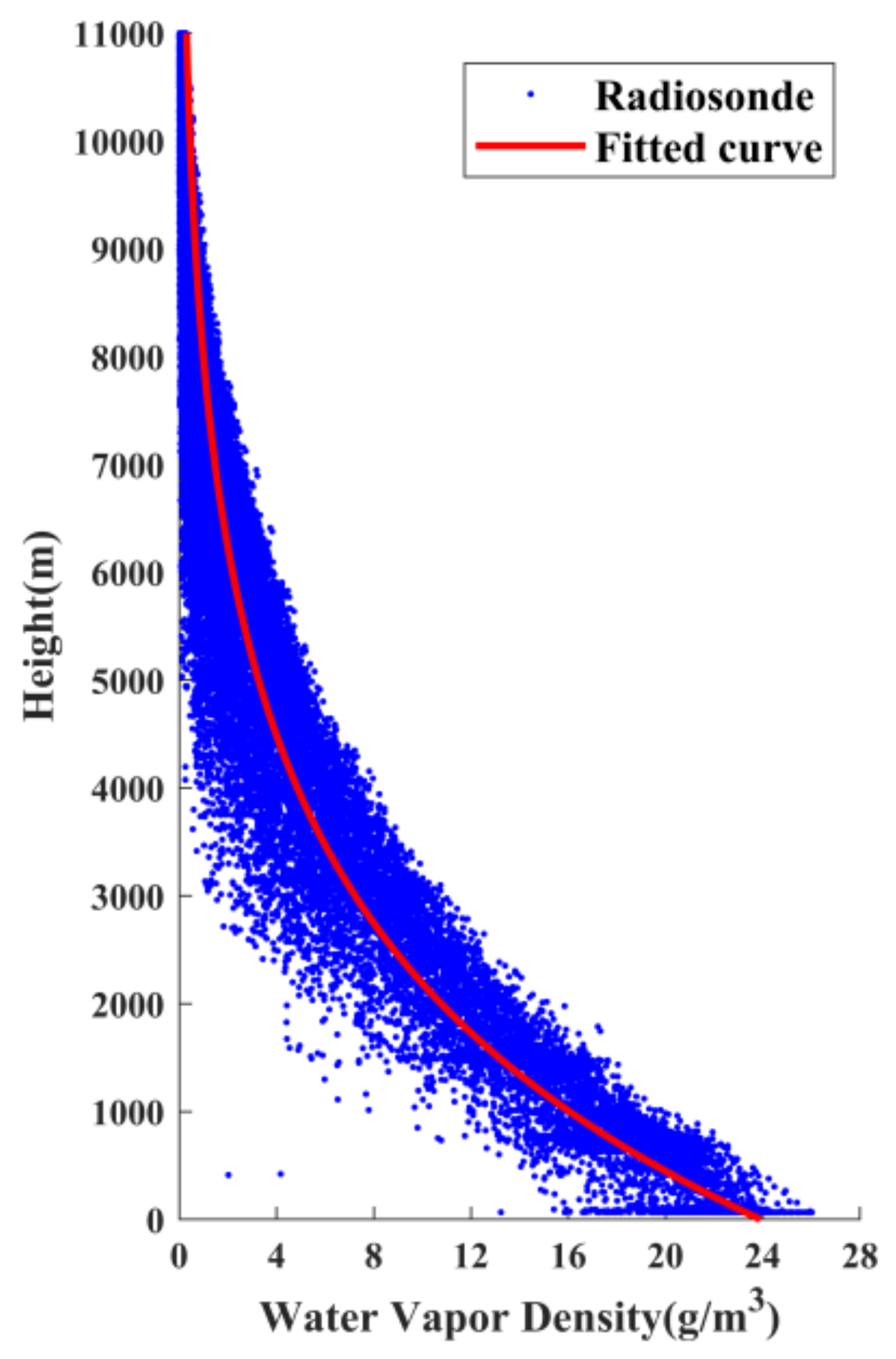
3.1. Modeling of Vertical Distribution Characteristics of Atmospheric Water Vapor
3.2. Adaptive Non-Uniform Exponential Stratification Method
4. Results and Validations
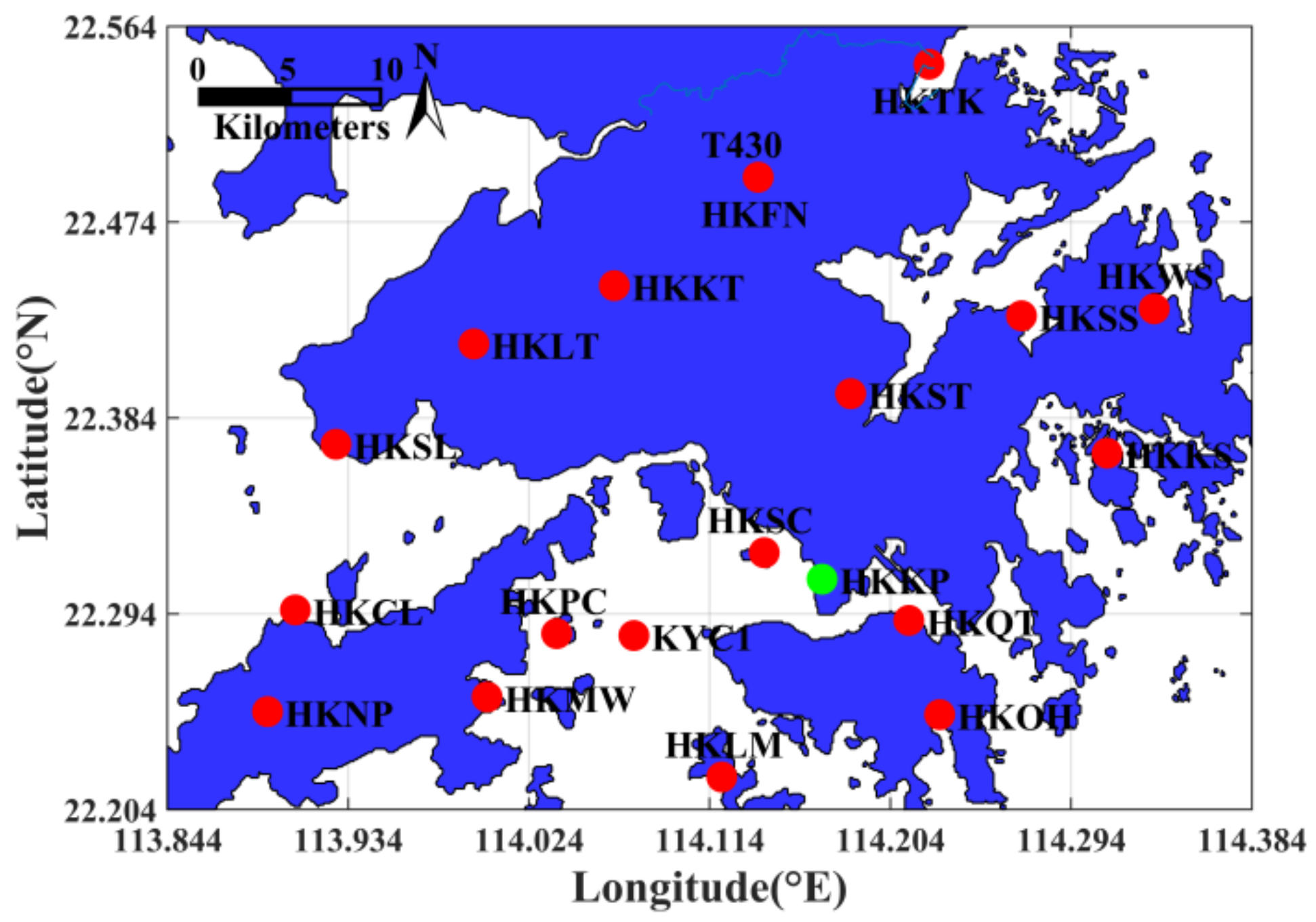
4.1. Processing Strategy
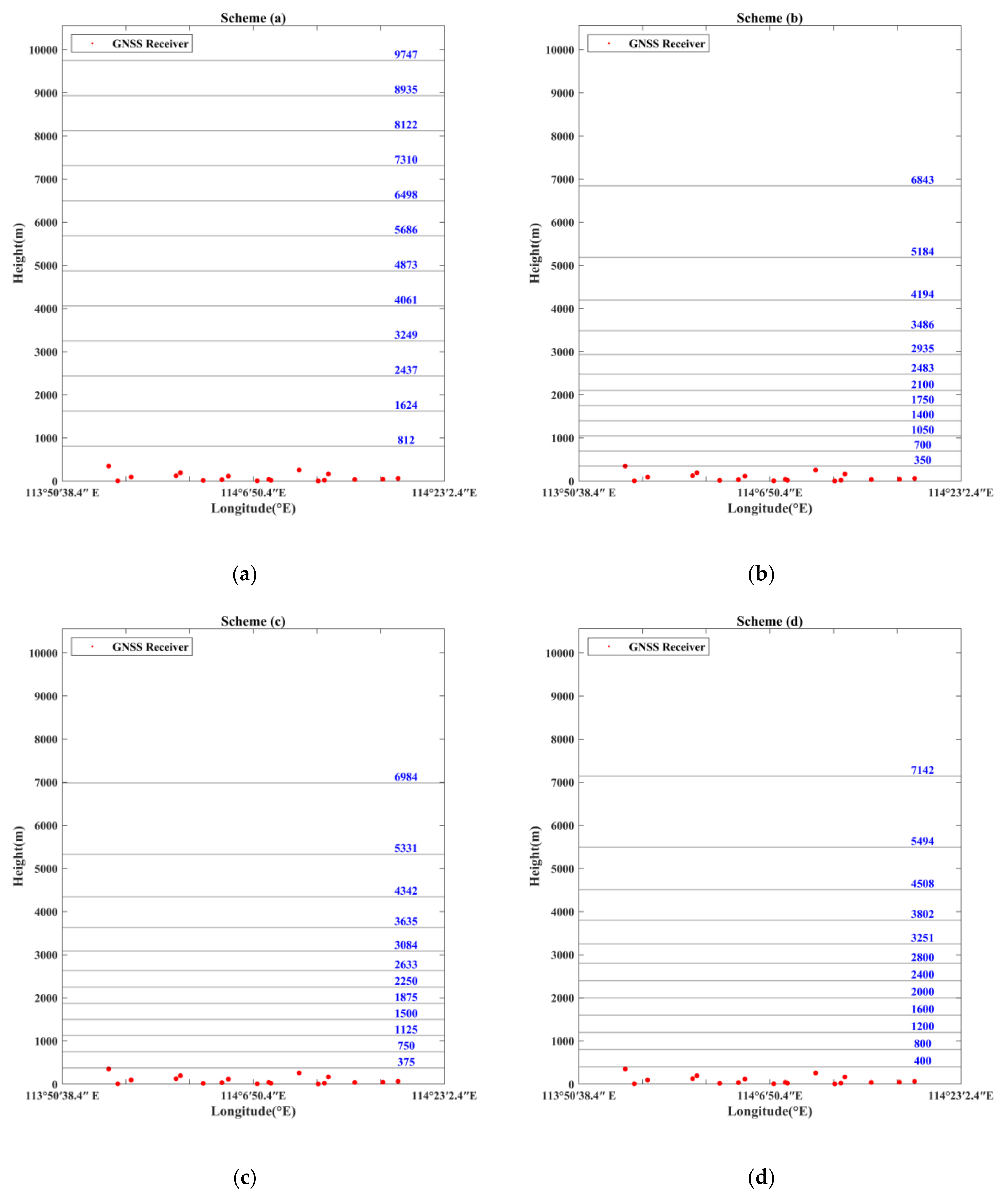
4.2. Vertical Stratification Strategy
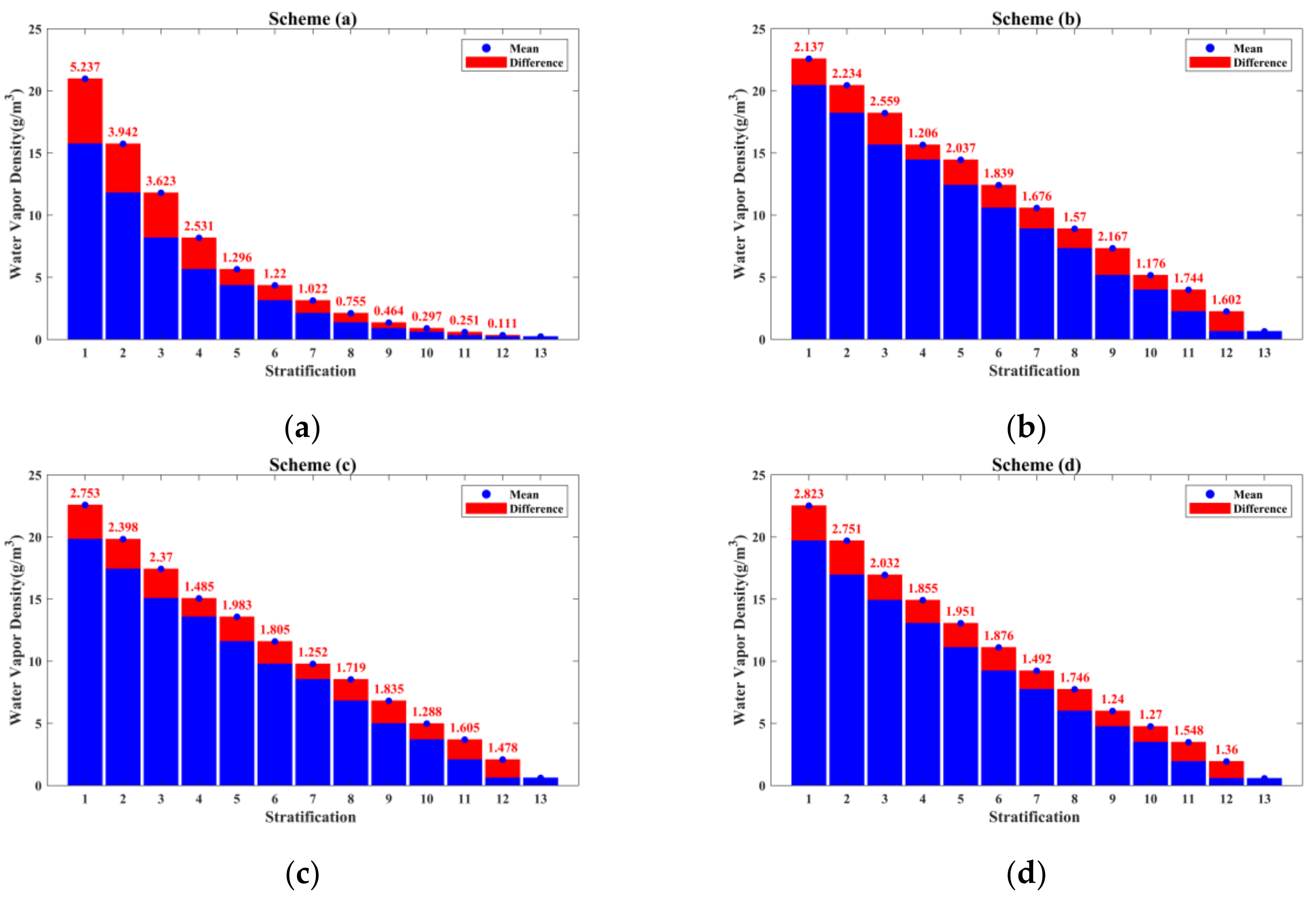
4.3. Tomographic Experiments and Evaluation of the ANES Approach
5. Discussion
6. Conclusions
Author Contributions
Funding
Institutional Review Board Statement
Informed Consent Statement
Data Availability Statement
Acknowledgments
Conflicts of Interest
References
- Bevis, M.; Businger, S.; Herring, T.A.; Rocken, C.; Anthes, R.A.; Ware, R.H. GPS meteorology: Remote sensing of atmospheric water vapor using the Global Positioning System. J. Geophys. Res. Atmos. 1992, 97, 15787–15801. [Google Scholar] [CrossRef]
- Baker, H.C.; Dodson, A.H.; Penna, N.T.; Higgins, M.; Offiler, D. Ground-based GPS water vapour estimation: Potential for meteorological forecasting. J. Atmos. Solar-Terr. Phys. 2001, 63, 1305–1314. [Google Scholar] [CrossRef]
- Elósegui, P.; Ruis, A.; Davis, J.L.; Ruffini, G.; Kruse, L.P. An experiment for estimation of the spatial and temporal variations of water vapor using GPS data. Phys. Chem. Earth 1998, 23, 125–130. [Google Scholar] [CrossRef]
- Rocken, C.; Hove, T.V.; Johnson, J.; Solheim, F.; Ware, R.; Bevis, M.; Businger, S. GPS/STORM-GPS sensing of atmospheric water vapor for meteorology. J. Atmos. Ocean. Technol. 1995, 12, 468–478. [Google Scholar] [CrossRef]
- Duan, J.; Bevis, M.; Fang, P.; Bock, Y.; Chiswell, S.; Businger, S.; Rocken, C.; Solheim, F.; Van, H.T.; Ware, R. GPS Meteorology: Direct estimation of the absolute value of precipitable water. J. Appl. Meteorol. 1996, 35, 830–838. [Google Scholar] [CrossRef] [Green Version]
- Baelen, J.V.; Aubagnac, J.P.; Dabas, A. Comparison of near-real time estimates of integrated water vapor derived with GPS, radiosondes, and microwave radiometer. J. Atmos. Ocean. Technol. 2005, 22, 201–210. [Google Scholar] [CrossRef]
- Emardson, T.R.; Elgered, G.; Johansson, J.M. Three months of continuous monitoring of atmospheric water vapor with a network of Global Positioning System receivers. J. Geophys. Res. Atmos. 1998, 103, 1807–1820. [Google Scholar] [CrossRef]
- Jin, S.; Luo, O.F. Variability and climatology of PWV from global 13-year GPS observations. IEEE Trans. Geosci. Remote Sens. 2009, 47, 1918–1924. [Google Scholar] [CrossRef]
- Kursinski, R.; Hajj, G.A.; Leroy, S.S.; Herman, B. The GPS radio occultation technique. Terr. Atmos. Ocean. Sci. 2001, 11, 53. [Google Scholar] [CrossRef] [Green Version]
- Flores, A.; Ruffini, G.; Rius, A. 4D tropospheric tomography using GPS slant wet delays. Ann. Geophys. 2000, 18, 223–234. [Google Scholar] [CrossRef]
- Hirahara, K. Local GPS tropospheric tomography. Earth Planets Space 2000, 52, 935–939. [Google Scholar] [CrossRef] [Green Version]
- Seko, H.; Shimada, S.; Nakamura, H.; Kato, T. Three-dimensional distribution of water vapor estimated from tropospheric delay of GPS data in a mesoscale precipitation system of the Baiu front. Earth Planets Space 2000, 52, 927–933. [Google Scholar] [CrossRef] [Green Version]
- Troller, M.; Geiger, A.; Brockmann, E.; Bettems, J.M.; Kahle, H.G. Tomographic determination of the spatial distribution of water vapor using GPS observations. Adv. Space Res. 2006, 37, 2211–2217. [Google Scholar] [CrossRef]
- Bender, M.; Dick, G.; Ge, M.; Deng, Z.; Wickert, J.; Kahle, H.G.; Raabe, A.; Tetzlaff, G. Development of a GNSS water vapour tomography system using algebraic reconstruction techniques. Adv. Space Res. 2011, 47, 1704–1720. [Google Scholar] [CrossRef] [Green Version]
- Chen, B.; Liu, Z. Voxel-optimized regional water vapor tomography and comparison with radiosonde and numerical weather model. J. Geodesy 2014, 88, 691–703. [Google Scholar] [CrossRef]
- Yao, Y.; Zhao, Q. Maximally using GPS observation for water vapor tomography. IEEE Trans. Geosci. Remote Sens. 2016, 54, 7185–7196. [Google Scholar] [CrossRef]
- Bao, Z.; Fan, Q.; Yao, Y.; Xu, C.; Li, X. An improved tomography approach based on adaptive smoothing and ground meteorological observations. Remote Sens. 2017, 9, 886. [Google Scholar] [CrossRef] [Green Version]
- Guo, J.; Fei, Y.; Shi, J.; Xu, C. An optimal weighting method of global positioning system (GPS) troposphere tomography. IEEE J. Sel. Top. Appl. Earth Obs. Remote Sens. 2017, 9, 5880–5887. [Google Scholar] [CrossRef]
- Xia, P.; Cai, C.; Liu, Z. GNSS troposphere tomography based on two-step reconstructions using GPS observations and COSMIC profiles. Ann. Geophys. 2013, 31, 1805–1815. [Google Scholar] [CrossRef] [Green Version]
- Zhao, Q.; Yao, Y.; Yao, W. Troposphere water vapour tomography: A horizontal parameterised approach. Remote Sens. 2018, 10, 1241. [Google Scholar] [CrossRef] [Green Version]
- Ding, N.; Zhang, S.; Zhang, Q. New parameterized model for GPS water vapor tomography. Ann. Geophys. 2017, 35, 311–323. [Google Scholar] [CrossRef] [Green Version]
- Jiang, P.; Ye, S.R.; Liu, Y.Y.; Zhang, J.J.; Xia, P.F. Near real-time water vapor tomography using ground-based GPS and meteorological data: Long-term experiment in Hong Kong. Ann. Geophys. 2014, 32, 911–923. [Google Scholar] [CrossRef] [Green Version]
- Perler, D.; Geiger, A.; Hurter, F. 4D GPS water vapor tomography: New parameterized approaches. J. Geod. 2011, 85, 539–550. [Google Scholar] [CrossRef] [Green Version]
- Liu, Y.; Chen, Y.; Liu, J. Determination of weighed mean tropospheric temperature using ground meteorological measurements. Geo-Spat. Inf. Sci. 2001, 4, 14–18. [Google Scholar] [CrossRef]
- Böhm, J.; Niell, A.; Tregoning, P.; Schuh, H. Global Mapping Function (GMF): A new empirical mapping function based on numerical weather model data. Geophys. Res. Lett. 2006, 33, 1–4. [Google Scholar] [CrossRef] [Green Version]
- Saastamoinen, J.H. Atmospheric correction for the troposphere and the stratosphere in radio ranging satellites. Use Artif. Satell. Geod. 1972, 15, 247–251. [Google Scholar] [CrossRef]
- Skone, S.; Hoyle, V. Troposphere modeling in a regional GPS network. J. Glob. Position. Syst. 2005, 4, 230–2391. [Google Scholar] [CrossRef] [Green Version]
- Nilsson, T.; Gradinarsky, L. Water vapor tomography using GPS phase observations: Simulation results. IEEE Trans. Geosci. Remote Sens. 2006, 44, 2927–2941. [Google Scholar] [CrossRef]
- Bender, M.; Raabe, A. Preconditions to ground based GPS water vapour tomography. Ann. Geophys. 2007, 25, 1727–1734. [Google Scholar] [CrossRef]
- Wexler, A. Vapor pressure formulation for water in range 0 to 100°. A Revision. J. Res. Natl. Bur. Stand. Sect. A Phys. Chem. 1976, 80A, 775–785. [Google Scholar] [CrossRef]
- Adeyemi, B.; Joerg, S. Analysis of water vapor over Nigeria using radiosonde and satellite data. Appl. Meteorol. Clim. 2012, 51, 1855–1866. [Google Scholar] [CrossRef]
- Liu, Z.; Wong, M.S.; Nichol, J.; Chan, P.W. A multi-sensor study of water vapour from radiosonde, MODIS and AERONET: A case study of Hong Kong. Int. J. Climatol. 2013, 33, 109–120. [Google Scholar] [CrossRef] [Green Version]
- Ha, J.; Park, K.D.; Kim, K.; Kim, Y.H. Comparison of atmospheric water vapor profiles obtained by GPS, MWR, and radiosonde. Asia-Pac. J. Atmos. Sci. 2010, 46, 233–241. [Google Scholar] [CrossRef]
- Haji-Aghajany, S.; Amerian, Y. Hybrid regularized GPS tropospheric sensing using 3-D ray tracing technique. IEEE Geosci. Remote Sens. Lett. 2018, 15, 1475–1479. [Google Scholar] [CrossRef]
- Haji-Aghajany, S.; Amerian, Y.; Verhagen, S. B-spline function-based approach for GPS tropospheric tomography. GPS Solut. 2020, 24, 193–205. [Google Scholar] [CrossRef]
- Zhang, W.; Zhang, S.; Zheng, N.; Ding, N.; Liu, X. A new integrated method of GNSS and MODIS measurements for tropospheric water vapor tomography. GPS Solut. 2021, 25, 88. [Google Scholar] [CrossRef]
- Zhang, W.; Zhang, S.; Ding, N.; Zhao, Q. A tropospheric tomography method with a novel height factor model including two parts: Isotropic and anisotropic height factors. Remote Sens. 2020, 12, 1848. [Google Scholar] [CrossRef]


| Name of the Strategy | Setting of the Strategy |
|---|---|
| Cut-off elevation angle | 15° |
| Auxiliary IGS stations | BJFS, CHAN, USUD |
| Sampling interval for the GPS data | 30 s |
| Tropospheric delay correction model | Saastamoinen |
| Mapping function | VMF1 |
| Ocean tidal model | FES2004 |
| Solid tide model | IERS2003 |
| Interval of gradient parameters | 2 h |
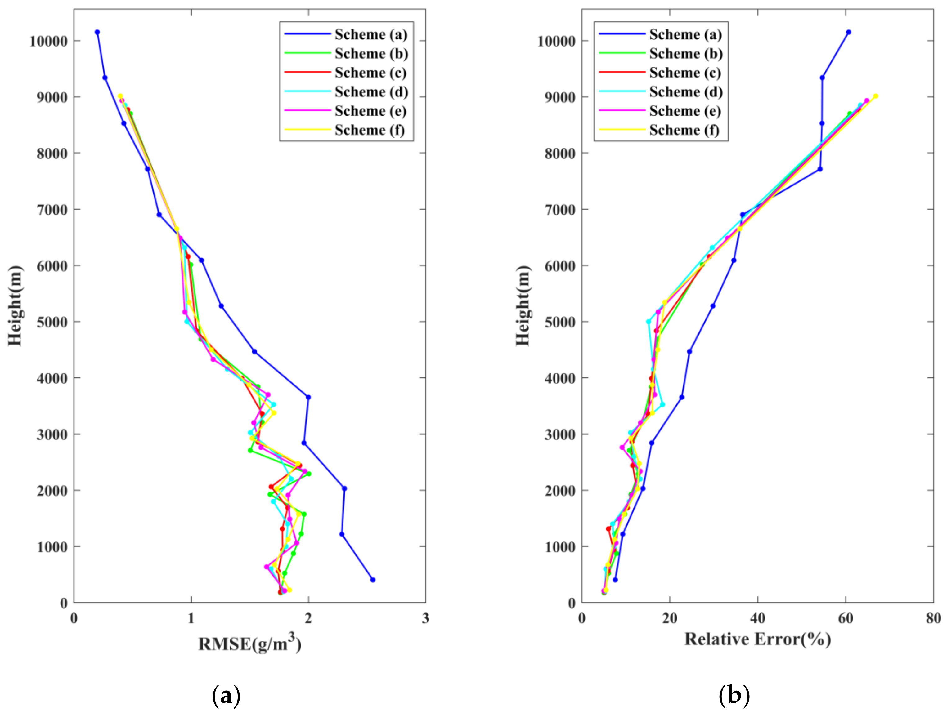
| Statistics | Scheme (a) | Scheme (b) | Scheme (c) | Scheme (d) | Scheme (e) | Scheme (f) |
|---|---|---|---|---|---|---|
| RMSE (unit: g/m3) | 1.321 | 1.104 | 1.075 | 1.066 | 1.070 | 1.074 |
| Bias (unit: g/m3) | 0.167 | −0.07 | −0.104 | −0.09 | −0.08 | −0.07 |
| MAE (unit: g/m3) | 0.822 | 0.800 | 0.777 | 0.764 | 0.756 | 0.755 |
| Approach | Area | Duration | Number of GPS Stations | Horizontal Resolution | Vertical Stratification | RMSE (Unit: g/m3) | Percentage | |
|---|---|---|---|---|---|---|---|---|
| COMMON | IMPROVED | |||||||
| ANES (minimum height interval: 400 m) | Hong Kong | 31 days | 19 | 0.09° × 0.09° | ANES | 1.32 | 1.07 | 18.94% |
| Tikh-LSQR | Tehran | 10 days | 11 | 0.25° × 0.25° | Uniform (500 m; 1000 m) | 0.82 | 0.40 | 51.22% |
| LB-Tikh | Tehran | 10 days | 11 | 0.25° × 0.25° | Uniform (500 m; 1000 m) | 0.82 | 0.49 | 40.24% |
| Function-based | North America | 30 days | 17 | 0.20° × 0.20° | Uniform (500 m; 1000 m) | 0.89 | 0.61 | 31.46% |
| Integration of MODIS measurements | Xuzhou (China) | 31 days | 5 | 0.13° × 0.14° | Non-uniform | 2.74 | 2.53 | 7.66% |
| HFM | Hong Kong | 31 days | 9 | 0.09° × 0.08° | Non-uniform | 1.63 | 1.13 | 30.67% |
| Voxel-optimized | Hong Kong | 20 days | 12 | 0.09° × 0.09° | Non-uniform | 1.38 | 1.23 | 10.87% |
Publisher’s Note: MDPI stays neutral with regard to jurisdictional claims in published maps and institutional affiliations. |
© 2021 by the authors. Licensee MDPI, Basel, Switzerland. This article is an open access article distributed under the terms and conditions of the Creative Commons Attribution (CC BY) license (https://creativecommons.org/licenses/by/4.0/).
Share and Cite
Wang, H.; Ding, N.; Zhang, W. An Adaptive Non-Uniform Vertical Stratification Method for Troposphere Water Vapor Tomography. Remote Sens. 2021, 13, 3818. https://doi.org/10.3390/rs13193818
Wang H, Ding N, Zhang W. An Adaptive Non-Uniform Vertical Stratification Method for Troposphere Water Vapor Tomography. Remote Sensing. 2021; 13(19):3818. https://doi.org/10.3390/rs13193818
Chicago/Turabian StyleWang, Hao, Nan Ding, and Wenyuan Zhang. 2021. "An Adaptive Non-Uniform Vertical Stratification Method for Troposphere Water Vapor Tomography" Remote Sensing 13, no. 19: 3818. https://doi.org/10.3390/rs13193818