Technical Note

Accuracy of Global Ionosphere Maps in Relation to Their Time Interval

by
Beata Milanowska
*,
Paweł Wielgosz
,
Anna Krypiak-Gregorczyk
and
Wojciech Jarmołowski
Faculty of Geoengineering, University of Warmia and Mazury in Olsztyn, 10-719 Olsztyn, Poland
*
Author to whom correspondence should be addressed.
Remote Sens. 2021, 13(18), 3552; https://doi.org/10.3390/rs13183552
Submission received: 27 July 2021 / Revised: 28 August 2021 / Accepted: 3 September 2021 / Published: 7 September 2021
(This article belongs to the Special Issue GNSS Atmospheric Modelling)

Abstract

:
Global ionosphere maps (GIMs) representing ionospheric total electron content (TEC) are applicable in many scientific and engineering applications. However, the GIMs provided by seven Ionosphere Associated Analysis Centers (IAACs) are generated with different temporal resolutions and using different modeling techniques. In this study, we focused on the influence of map time interval on the empirical accuracy of these ionospheric products. We investigated performance of the high-resolution GIMs during high (2014) and low (2018) solar activity periods as well as under geomagnetic storms (19 February 2014 and 17 March 2015). In each of the analyzed periods, GIMs were also assessed over different geomagnetic latitudes. For the evaluation, we used direct comparison of GIM-derived slant TEC (STEC) with dual-frequency GNSS observations obtained from 18 globally distributed stations. In order to perform a comprehensive study, we also evaluated GIMs with respect to altimetry-derived vertical TEC (VTEC) obtained from the Jason-2 and Jason-3 satellites. The study confirmed the influence of GIMs time interval on the provided TEC accuracy, which was particularly evident during high solar activity, geomagnetic storms, and also at low latitudes. The results show that 120-min interval contributes significantly to the accuracy degradation, whereas 60-min one is sufficient to maintain TEC accuracy.
Keywords:
TEC; GIM; time interval; GNSS

1. Introduction

Over the last decades, the Global Navigation Satellite System (GNSS) has become a valuable tool for remote sensing of the ionosphere. Using dual-frequency measurements, one of the most important ionospheric quantities, the total electron content (TEC), may be obtained. This ionospheric TEC is usually provided in the IONosphere EXchange format (IONEX) in the form of global ionosphere maps (GIMs). Currently, seven Ionosphere Associated Analysis Centers (IAACs) of the International GNSS Service (IGS) generate their own GIMs [1]. These ionospheric products are commonly used in many practical and scientific applications, like precise positioning or space weather studies. For example, GNSS users require ionospheric corrections to improve their position estimates [2,3,4,5]. Moreover, space weather and geophysical studies are often based on GIM data [6,7,8].
Since there is a wide range of the above-mentioned engineering and geophysical applications of GIMs, it is essential to validate empirical accuracy of the ionospheric products. So far, several studies have been published in the context of the GIMs performance. This kind of research is based on the comparison of the TEC derived from the IAAC models with selected reference TEC values. Given that GIMs are global products, two complementary methods are recommended to investigate their quality: (1) direct comparison to relative slant TEC (STEC) from dual-frequency GNSS observations, and (2) comparison to vertical TEC (VTEC) derived from dual-frequency satellite altimeter measurements above the oceans [9]. As is well-known, the ionosphere is primarily driven by solar and geomagnetic conditions. Therefore, GIM performance is generally studied in relation to different solar activity levels as well as under different geomagnetic conditions [10,11,12]. Since the ionosphere is characterized by spatial variability, the assessment of GIM often divides the Earth into a few latitude-dependent regions [13].
It should be noted that ionosphere temporal variability may have a noticeable impact on GIM accuracy. In the beginning of the IGS Ionosphere Working Group activity, all contributing IAACs produced GIMs at a 120-min interval. Over the years, some of the centers have started to provide products with higher temporal resolution. Currently, the IAACs provide GIMs with intervals ranging from 30 to 120 min. Besides the IGS products, the Ion-SAT group from the Polytechnic University of Catalonia (UPC) generates GIM (UQRG) with a very high resolution of 15 min [14]. However, the relation of GIMs interval to their accuracy is still under-researched. One of the recent studies on GIM performance that includes GIM interval analysis was published by Roma-Dollase et al. [15]. This analysis, based on UPC GIMs, was performed in relation to VTEC altimeter data. Liu et al. [16] presented the study focusing entirely on the influence of the temporal resolution, however again only UPC GIMs were analyzed. Besides these two well-known investigations, the studies on GIM performance usually do not consider their temporal resolution. Therefore, we propose a comprehensive study focused on the influence of GIM interval on performance of IAAC final ionospheric products. In our study, IAAC GIMs and UQRG GIM were assessed with GNSS and altimetry-derived TEC during selected low and high solar activity periods, as well as during geomagnetic storms, and also over different geomagnetic latitudes.

2. Materials and Methods

To analyze GIMs under different solar and geomagnetic conditions, we selected four periods:
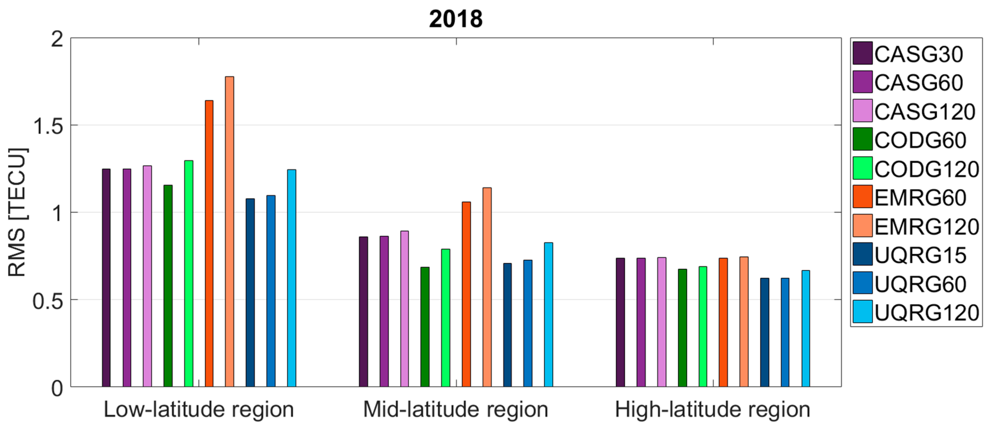
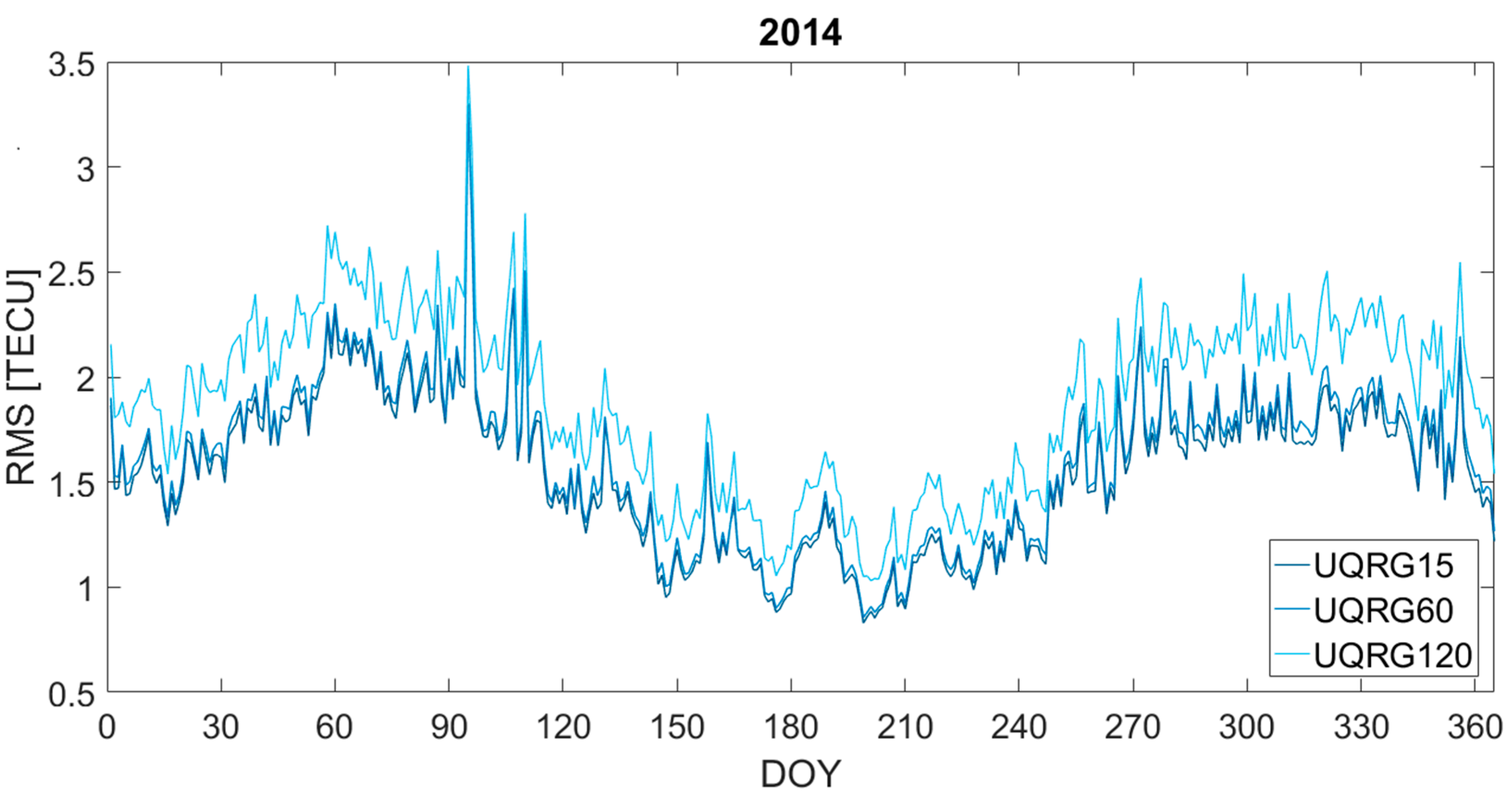
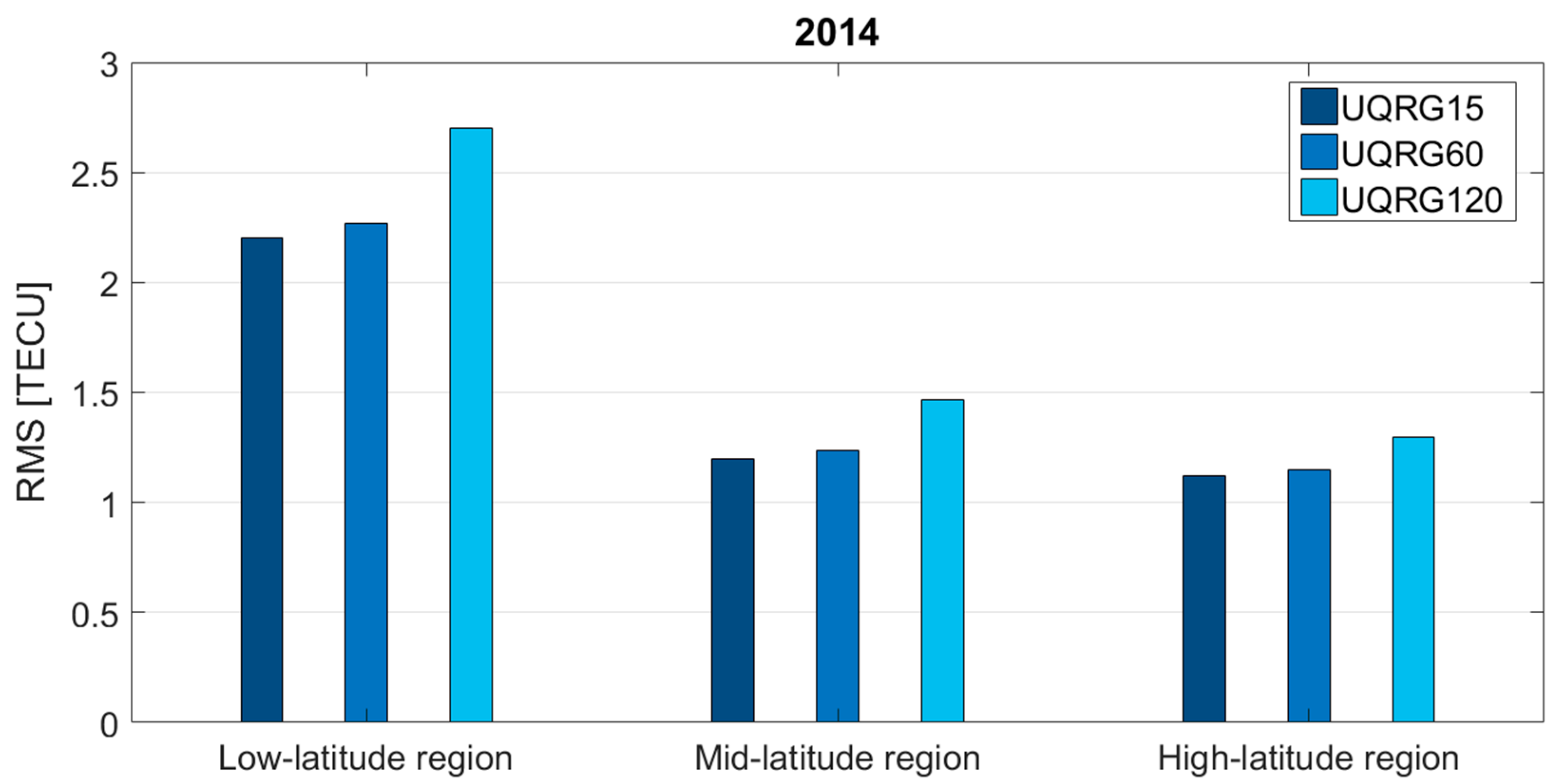
  • Year 2014, representing high solar activity period (F10.7 index ranged from 89 to 253 sfu);
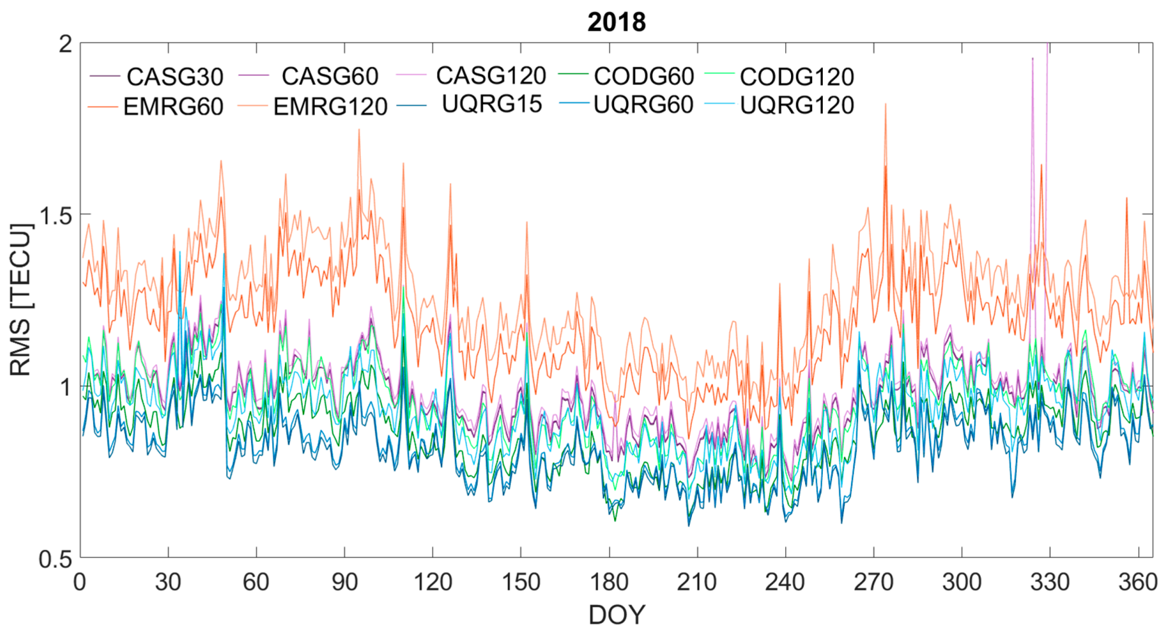
  • Year 2018, representing low solar activity period (F10.7 index ranged from 65 to 85 sfu);
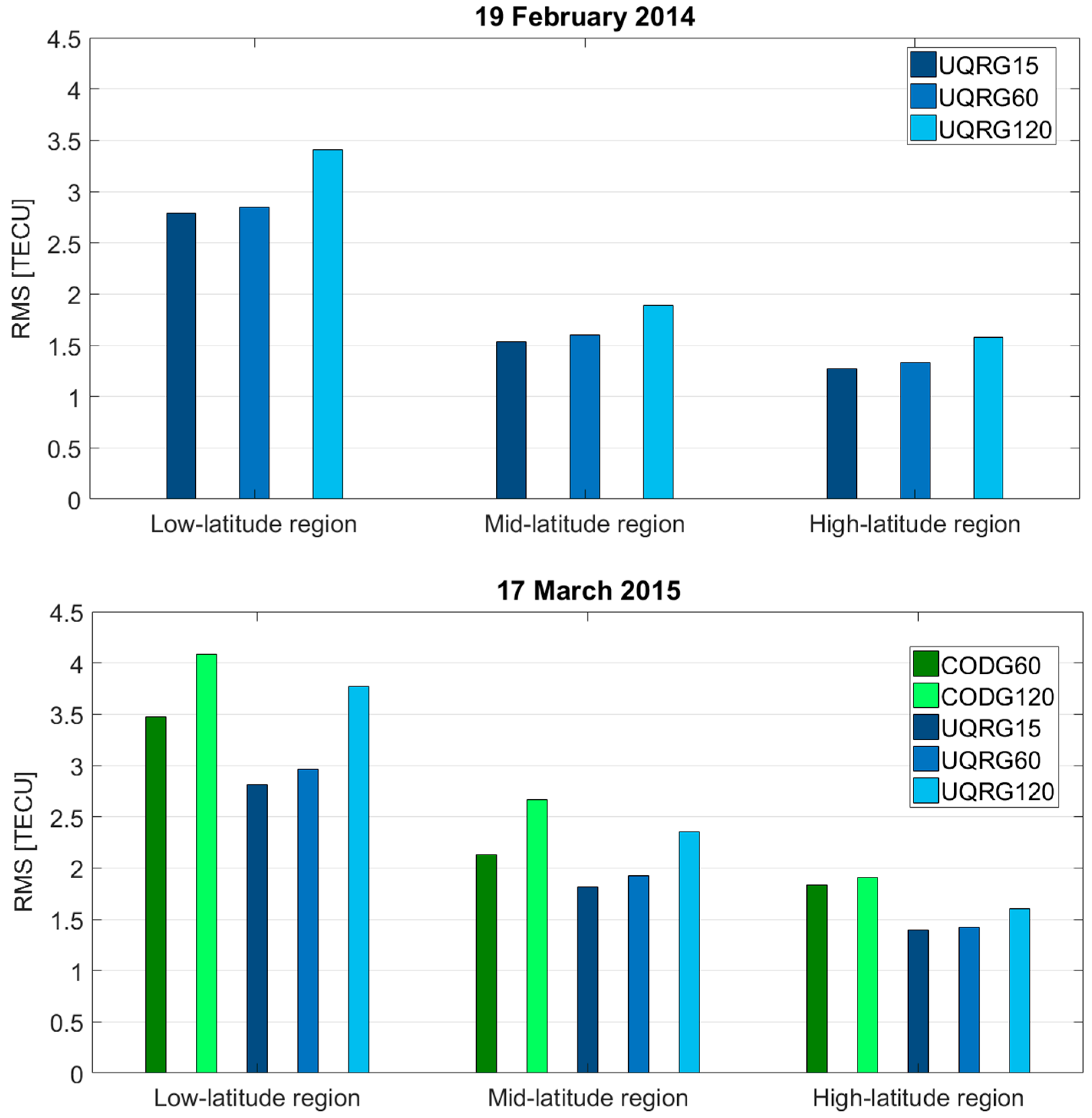
  • the first case study during geomagnetic storm on 19 February 2014 (max Kp = 6+);
  • the second case study during the St. Patrick’s Day geomagnetic storm on 17 March 2015 (max Kp = 8−).
In each of these periods, GIMs were also analyzed with respect to three distinctive geographic regions. The analysis was performed for (1) low geomagnetic latitudes covering equatorial region (from 30°S to 30°N), (2) mid-latitude region (from 30° to 60° in both hemispheres), and (3) high latitudes covering polar and auroral zones (from 60° to 90° in both hemispheres). For the investigation, we chose the final GIMs, providing grids of VTEC values with spatial resolution of 2.5° × 5° in the latitude and longitude, respectively. In our study, we tested three IAAC GIMs and also UQRG GIM, since these GIMs are available with higher temporal resolution than standard 120 min (see Table 1). Each product was analyzed with its nominal temporal resolution, and additionally with resolution reduced to 60 and 120 min.
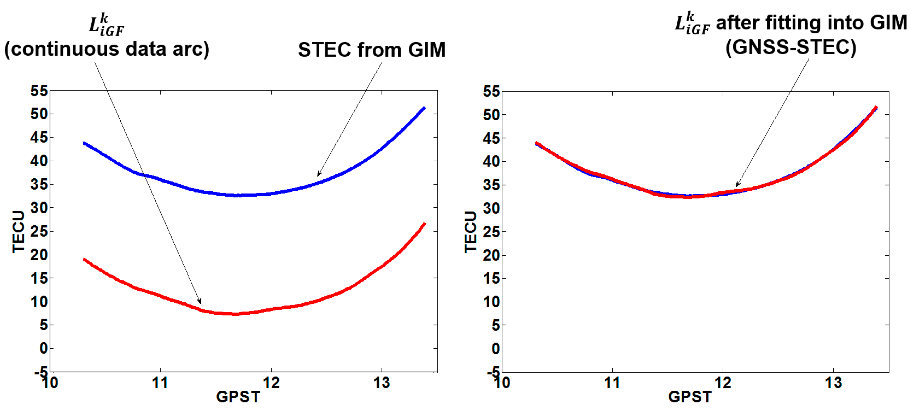
In order to comprehensively evaluate the analyzed models, we made a comparison of GIM-derived TEC with two independent reference TEC data sources: STEC from ground GNSS observations (GNSS-STEC) and VTEC from altimeter measurements (Alt-VTEC) over the oceans. The former reference data are based on the precise carrier phase L1 and L2 observables. These observables form the geometry-free linear combination ( L i G F k ) that is used to extract STEC data along phase continuous data arc between receiver i and satellite k. This is the most precise evaluation method often called self-consistency analysis, and according to Feltens et al. [20] its accuracy is of about 0.1 TECU. In this study, we used the approach published by Krypiak-Gregorczyk et al. [21], where GNSS geometry-free data are fitted into GIM-derived STEC, and post-fit residuals (RMS) are analyzed (Figure 1). Namely, (1) L i G F k combination is created for each continuous data arc cleaned from gaps and cycle slips, (2) STEC from GIMs is calculated for the same data arc at ionosphere piercing points (IPP), (3) L i G F k is fitted into GIM-derived STEC resulting in GNSS-STEC, (4) post-fit residuals are created, and (5) their RMS is calculated as a GIMs accuracy metric. As IPP locations change with every observational epoch, this approach allows for testing GIMs in both space and time.
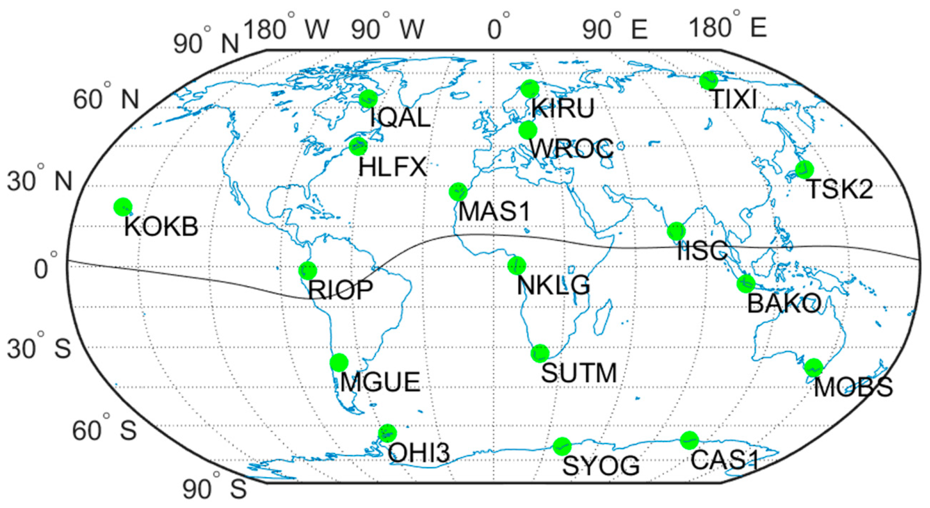
For this approach, 18 globally distributed stations were selected (Figure 2). The calculations were carried out using the GPS data with 30-s intervals and 25° elevation cut-off. In the case of GIMs data, VTEC values were interpolated using a method recommended by Schaer et al. [22]. This approach is based on linear interpolation, and it is a function of latitude, longitude and time. Then the resulting VTEC was converted to STEC using the standard single layer model (SLM) mapping function (h = 450 km and α = 1, [18]).
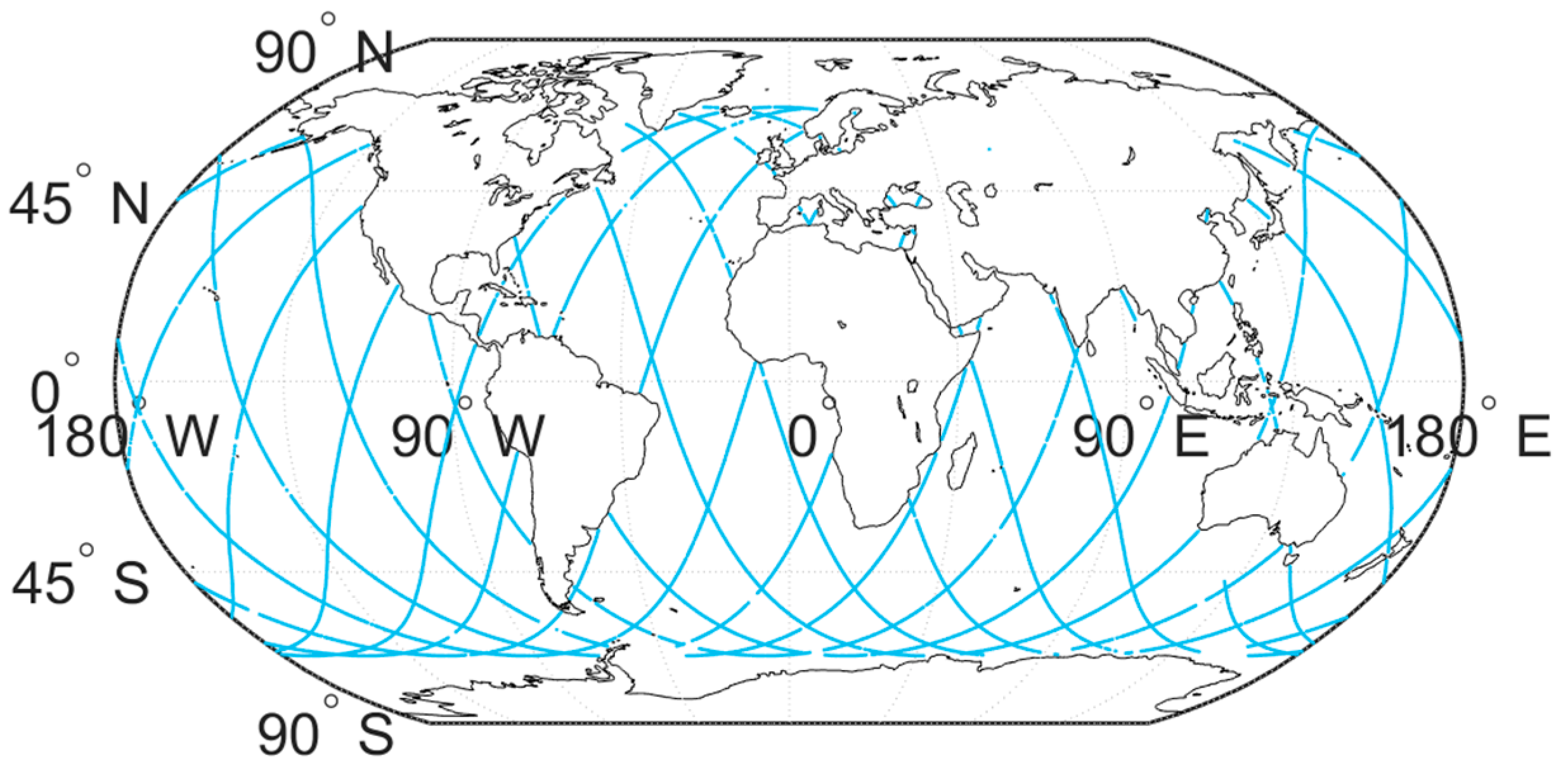
The latter data source uses altimeter measurements for GIM evaluation. Dual-frequency altimeters enable the determination of reference VTEC, which is a unique and independent source of TEC data, as it provides VTEC directly with no mapping function need [9]. This data are limited to sea/ocean regions (Figure 3), hence allowing GIM evaluation in areas far from the GNSS stations. In this study, we selected data from Jason-2 and Jason-3 satellites. More detailed description of VTEC data extraction from altimeter measurement can be found in Imel [23]. One should keep in mind that altimetry-derived VTEC needs to be preprocessed (filtered and smoothed) to serve as a reference for GIM evaluation. Therefore, we used the median with a window of 80 s, which filters altimetry VTEC in low-pass mode, removing high-frequency noise and making it more comparable to the upper frequencies of GIMs. Applying this process results in Alt-VTEC accuracy of about 1 TECU [9]. To achieve consistency with GIM VTEC, altimetry data were complemented with remaining plasmaspheric VTEC above the satellite orbital height (over ~1300 km). For this reason, we used model-derived plasmaspheric VTEC from the NeQuick-2 empirical model [24]. Our earlier study shows that the application of plasmaspheric VTEC improved the comparison results by even 11% [12]. Moreover, VTEC data are also affected by unknown instrumental bias. To reduce this bias, our analysis was based on standard deviation (STD) of differences between Alt-VTEC and GIM VTEC.

3. Results

Using the two aforementioned evaluation methods, we investigated the accuracy of GIMs during low and high solar activity periods as well as during geomagnetic storms. When discussing the results, we use GIM labels consisting of the 4-letter GIM code and the evaluated temporal resolution in minutes, e.g., ‘CASG30’ in the case of the CASG maps with 30-min interval.

3.1. Low Solar Activity

To study the impact of GIMs interval during low solar activity, we analyzed four available high-rate maps (Table 1) over the whole year of 2018. This year corresponds to the solar minimum of the 24th Solar Activity Cycle, when daily F10.7 solar flux does not exceed 85 sfu [25]. Daily RMS distribution (mean from all PRNs and stations) derived from GNSS-STEC comparisons is shown in Figure 4. For each of the tested GIMs, it can be observed that reducing temporal resolution increases resulting daily RMS. As shown in Table 2, annual RMS increased from about 2 to 14% for CASG and UQRG, respectively, when comparing the nominal and 120-min intervals. The lowest RMS was obtained for UQRG15 maps, while the highest one was observed for EMRG120 maps.
The performance of GIMs was also analyzed over different geomagnetic regions. Since the influence of the interval on the altimeter data are less pronounced, here we focus only on the GNSS-STEC analysis. We evaluated the resulting annual RMS for each of the three selected regions (see Figure 5). One can observe that the difference in GIMs accuracy between nominal and reduced temporal resolution increases as they get closer to the equator. This may indicate that higher TEC and its gradients over the equatorial anomaly require higher temporal resolution to be properly represented by a GIM. However, this phenomenon is not so clearly visible for CASG GIM.
The second evaluation method based on Alt-VTEC data confirms the influence of GIM interval on TEC accuracy. However, the differences of the annual STDs are usually less than 2% during the low solar activity period (Table 3). The lowest STD was obtained for UQRG15 maps, while the highest one was observed for EMRG60 maps. It is worth noting that the annual STD worsened only for CODG and UQRG, while it improved slightly for CASG and EMRG. This weaker effect, comparing to GNSS-STEC results, may come from the fact that the reference Alt-VTEC is a filtered product (median).

3.2. High Solar Activity

During the second analyzed period covering the solar maximum (2014), the daily solar flux index ranged from 89 to 253 sfu. This confirms much greater solar radiation energy input compared to 2018 with max F10.7 index = 85 sfu. Unfortunately, during this period only UQRG GIM produced high resolution maps with a time interval of 15 min, whereas IAAC GIMs provided maps with 120-min time resolution. In our analysis, the nominal interval of the UQRG model was reduced to 60 and 120 min. As can be seen in Figure 6, increasing the interval clearly raised the daily RMS. Similar to 2018’s results, this is particularly evident for the ‘UQRG120’ product. The annual RMS increased by about 3% and 21% for ‘UQRG60’ and ‘UQRG120’, respectively (Table 4). This effect is greater than in 2018 indicating that the impact of the GIM time interval is more significant during high solar activity.
In 2014, the performance of UQRG GIM was also analyzed over different geomagnetic regions with the use of GNSS-STEC data (Figure 7). The highest annual RMS in each analyzed region was obtained for a 120-min interval, reaching from 1.30 to 2.70 TECU. The RMS for this interval was about 18% higher than for a 60-min interval. As well as in 2018, the greatest impact of reducing the temporal resolution is visible in the low-latitude region.
In the context of Alt-VTEC comparisons, the influence of the temporal resolution was clearly noticed for the ‘UQRG120’ (Table 5). Indeed, the annual STD increased by about 6% indicating that during high solar activity the GIM time interval has a more noticeable influence on TEC accuracy. Note that the STD increase is 3.5 times higher than during the low solar activity period. Even though the altimetry tests show smaller accuracy change (in %) than the GNSS-STEC comparisons, the accuracy dependence on time interval is also confirmed.

3.3. Geomagnetic Storms

As it is known, the accuracy of GIMs depends on the solar activity level as well as geomagnetic conditions. In order to investigate the impact of the map interval under disturbed conditions, we selected two geomagnetic storms: on 19 February 2014 and on 17 March 2015 (St. Patrick’s Day Storm), with max Kp amounting to 6+ and 8−, respectively. Due to the limited availability of high-resolution GIMs, we analyzed the UQRG model during both storms and CODG GIM during St. Patrick’s Day storm. The results of GNSS-STEC comparisons for both storms are presented in Table 6. During the storm of 19 February 2014, the daily RMS for UQRG is clearly higher than the annual one in 2014 (see Table 4). During the storm of 17 March 2015, the increase in daily RMS is even greater despite the lower solar activity. When reducing the temporal resolution to 120 min, the daily RMS increased by almost 23% for UQRG GIM on 19 February, and during St. Patrick’s Day storm by around 17% and 29% for CODG and UQRG, respectively (see Table 6). For the UQRG GIM, the nominal interval was also increased to 60 min. The resulting daily RMS increased up to ~3 and 5% on 19 February and 17 March, respectively. As in previous cases, this reduction has a minor impact on GIM accuracy. Comparing the results obtained for the UQRG model during both storms, it can be concluded that the more severe storm, the greater influence of the temporal resolution on GIMs accuracy.
During selected geomagnetic storms, the self-consistency analysis (GNSS-STEC) over three geomagnetic regions shows similar tendencies as in the analysis during the two solar activity periods (Figure 8). Firstly, the 120-min interval has the largest disadvantageous impact on GIMs accuracy in each of the analyzed regions. Secondly, in the low-latitude region, the influence of temporal resolution is more clearly visible. However, this impact is even greater during geomagnetic storms.
Table 7 presents further storm-time analysis based on Alt-VTEC comparisons. However, the impact of the increased interval during geomagnetic storms is not as strong as in the case of the comparisons to GNSS-STEC. Nevertheless, during St. Patrick’s Day storm, both analyzed GIMs have worse accuracy when their interval is increased to 60/120 min. During this storm, the largest increase in the daily STD (by ~9%) was obtained for UQRG120 when its temporal resolution was decreased eightfold. This indicates that Alt-VTEC shows the same trends as GNSS-STEC in GIM interval analysis.

4. Conclusions

This study confirmed the influence of GIMs temporal resolution on TEC accuracy. Indeed, based on GNSS-STEC and Alt-VTEC analysis, this influence is clearly correlated with the phenomena that drive the ionosphere, such as solar and geomagnetic conditions. It can be observed that the accuracy degradation is the highest for the 120-min interval. In addition, the influence of temporal resolution is the most clearly visible in low-latitude region. This may indicate that higher TEC and its gradients existing over the equatorial anomaly require higher temporal resolution to be properly represented by GIMs. Moreover, the degradation of accuracy with increased map interval is even more evident during the geomagnetic storms. Looking at the results obtained for UQRG, it can be concluded that the more severe storm, the greater influence of the temporal resolution on GIMs accuracy.
In general, the interval of 60 min seems to be a good compromise between maps’ temporal resolution and their resulting accuracy and may be recommended in ionosphere GNSS remote sensing applications. This confirms suggestions presented by Liu et al. [16], who showed that temporal resolution higher than 1 h had a significant impact on accuracy degradation. Note, however, that this conclusion concerns the final IAAC products only. The quality of the real-time GIMs is still worse, even though they are provided with higher temporal resolutions [26].
Specific results show that the highest accuracy is obtained for the high-resolution UQRG15 maps, which are based on stochastic technique (kriging). It is interesting that in the case of CASG maps the interval has a lesser influence on the accuracy in comparison to other GIMs. This may suggest that the intrinsic interval of the underlying model is longer than 30 min.

Author Contributions

Conceptualization, P.W. and B.M.; software, B.M., A.K.-G. and W.J.; investigation, B.M., P.W., A.K.-G. and W.J.; writing—original draft preparation, B.M.; supervision, P.W. All authors have read and agreed to the published version of the manuscript.

Funding

This research was funded by the Polish National Center of Science (NCN), grant number UMO-2017/27/B/ST10/02219.

Data Availability Statement

Products containing ionosphere VTEC maps in the IONEX format and RINEX files are accessible from the NASA’s CDDIS sftp server (ftp://gdc.cddis.eosdis.nasa.gov/pub/). Altimetry data are accessible from the NOAA ftp server (ftp://ftp.nodc.noaa.gov/pub/). Kp index is accessible from the DTU Space ftp server (ftp.space.dtu.dk).

Conflicts of Interest

The authors declare no conflict of interest. The funders had no role in the design of the study; in the collection, analyses, or interpretation of data; in the writing of the manuscript, or in the decision to publish the results.

References

  1. Johnston, G.; Riddell, A.; Hausler, G. The international GNSS service. In Springer Handbook of Global Navigation Satellite Systems; Springer: Cham, Switzerland, 2017; pp. 967–982. [Google Scholar]
  2. Zhao, J.; Hernández-Pajares, M.; Li, Z.; Wang, N.; Yuan, H. Integrity Investigation of Global Ionospheric TEC Maps for High-Precision Positioning. J. Geod. 2021, 95, 1–15. [Google Scholar] [CrossRef]
  3. Grejner-Brzezinska, D.A.; Kashani, I.; Wielgosz, P.; Smith, D.A.; Spencer, P.S.; Robertson, D.S.; Mader, G.L. Efficiency and Reliability of Ambiguity Resolution in Network-Based Real-Time Kinematic GPS. J. Surv. Eng. 2007, 133, 56–65. [Google Scholar] [CrossRef]
  4. Ciećko, A.; Grunwald, G. Klobuchar, NeQuick G, and EGNOS Ionospheric Models for GPS/EGNOS Single-Frequency Positioning under 6–12 September 2017 Space Weather Events. Appl. Sci. 2020, 10, 1553. [Google Scholar] [CrossRef] [Green Version]
  5. Ghoddousi-Fard, R.; Lahaye, F. Evaluation of Single Frequency GPS Precise Point Positioning Assisted with External Ionosphere Sources. Adv. Space Res. 2016, 57, 2154–2166. [Google Scholar] [CrossRef]
  6. Azpilicueta, F.; Nava, B. A Different View of the Ionospheric Winter Anomaly. Adv. Space Res. 2021, 67, 150–162. [Google Scholar] [CrossRef]
  7. Ratovsky, K.G.; Klimenko, M.V.; Yasyukevich, Y.V.; Klimenko, V.V.; Vesnin, A.M. Statistical Analysis and Interpretation of High-, Mid-and Low-Latitude Responses in Regional Electron Content to Geomagnetic Storms. Atmosphere 2020, 11, 1308. [Google Scholar] [CrossRef]
  8. Shah, M.; Inyurt, S.; Ehsan, M.; Ahmed, A.; Shakir, M.; Ullah, S.; Iqbal, M.S. Seismo Ionospheric Anomalies in Turkey Associated with Mw≥ 6.0 Earthquakes Detected by GPS Stations and GIM TEC. Adv. Space Res. 2020, 65, 2540–2550. [Google Scholar] [CrossRef]
  9. Hernández-Pajares, M.; Roma-Dollase, D.; Krankowski, A.; García-Rigo, A.; Orús-Pérez, R. Methodology and Consistency of Slant and Vertical Assessments for Ionospheric Electron Content Models. J. Geod. 2017, 91, 1405–1414. [Google Scholar] [CrossRef]
  10. Liu, A.; Wang, N.; Li, Z.; Zhou, K.; Yuan, H. Validation of CAS’s Final Global Ionospheric Maps during Different Geomagnetic Activities from 2015 to 2017. Results Phys. 2018, 10, 481–486. [Google Scholar] [CrossRef]
  11. Krypiak-Gregorczyk, A. Ionosphere Response to Three Extreme Events Occurring near Spring Equinox in 2012, 2013 and 2015, Observed by Regional GNSS-TEC Model. J. Geod. 2019, 93, 931–951. [Google Scholar] [CrossRef] [Green Version]
  12. Wielgosz, P.; Milanowska, B.; Krypiak-Gregorczyk, A.; Jarmołowski, W. Validation of GNSS-Derived Global Ionosphere Maps for Different Solar Activity Levels: Case Studies for Years 2014 and 2018. GPS Solut. 2021, 25, 1–15. [Google Scholar] [CrossRef]
  13. Chen, P.; Liu, H.; Ma, Y.; Zheng, N. Accuracy and Consistency of Different Global Ionospheric Maps Released by IGS Ionosphere Associate Analysis Centers. Adv. Space Res. 2020, 65, 163–174. [Google Scholar] [CrossRef]
  14. Orús, R.; Hernández-Pajares, M.; Juan, J.M.; Sanz, J. Improvement of Global Ionospheric VTEC Maps by Using Kriging Interpolation Technique. J. Atmos. Solar-Terr. Phys. 2005, 67, 1598–1609. [Google Scholar] [CrossRef]
  15. Roma-Dollase, D.; Hernández-Pajares, M.; Krankowski, A.; Kotulak, K.; Ghoddousi-Fard, R.; Yuan, Y.; Li, Z.; Zhang, H.; Shi, C.; Wang, C.; et al. Consistency of Seven Different GNSS Global Ionospheric Mapping Techniques during One Solar Cycle. J. Geod. 2018, 92, 691–706. [Google Scholar] [CrossRef] [Green Version]
  16. Liu, Q.; Hernández-Pajares, M.; Lyu, H.; Goss, A. Influence of Temporal Resolution on the Performance of Global Ionospheric Maps. J. Geod. 2021, 95, 34. [Google Scholar] [CrossRef]
  17. Li, Z.; Yuan, Y.; Wang, N.; Hernandez-Pajares, M.; Huo, X. SHPTS: Towards a New Method for Generating Precise Global Ionospheric TEC Map Based on Spherical Harmonic and Generalized Trigonometric Series Functions. J. Geod. 2015, 89, 331–345. [Google Scholar] [CrossRef]
  18. Schaer, S. Mapping and Predicting the Earth’s Ionosphere Using the Global Positioning System; Springer Science: Cham, Switzerland, 1999. [Google Scholar]
  19. Ghoddousi-Fard, R.; Héroux, P.; Danskin, D.; Boteler, D. Developing a GPS TEC Mapping Service over Canada. Space Weather 2011, 9, 6. [Google Scholar] [CrossRef]
  20. Feltens, J.; Angling, M.; Jackson-Booth, N.; Jakowski, N.; Hoque, M.; Hernández-Pajares, M.; Aragón-Àngel, A.; Orús, R.; Zandbergen, R. Comparative Testing of Four Ionospheric Models Driven with GPS Measurements. Radio Sci. 2011, 46, 6. [Google Scholar] [CrossRef] [Green Version]
  21. Krypiak-Gregorczyk, A.; Wielgosz, P.; Borkowski, A. Ionosphere Model for European Region Based on Multi-GNSS Data and TPS Interpolation. Remote Sens. 2017, 9, 1221. [Google Scholar] [CrossRef] [Green Version]
  22. Schaer, S.; Gurtner, W.; Feltens, J. IONEX: The Ionosphere Map Exchange Format Version 1. In Proceedings of the IGS AC Workshop, Darmstadt, Germany, 9–11 February 1998; Available online: https://bit.ly/3zH1Trd (accessed on 20 July 2021).
  23. Imel, D.A. Evaluation of the TOPEX/POSEIDON Dual-Frequency Ionosphere Correction. J. Geophys. Res. 1994, 99, 24895–24906. [Google Scholar] [CrossRef]
  24. Nava, B.; Coisson, P.; Radicella, S.M. A New Version of the NeQuick Ionosphere Electron Density Model. J. Atmos. Solar-Terr. Phys. 2008, 70, 1856–1862. [Google Scholar] [CrossRef]
  25. Perrone, L.; Franceschi, G.D. Solar, Ionospheric and Geomagnetic Indices. Ann. Geophys. 1998, 41, 5–6. [Google Scholar] [CrossRef]
  26. Li, Z.; Wang, N.; Hernández-Pajares, M.; Yuan, Y.; Krankowski, A.; Liu, A.; Zha, J.; García-Rigo, A.; Roma-Dollase, D.; Yang, H.; et al. IGS Real-Time Service for Global Ionospheric Total Electron Content Modeling. J. Geod. 2020, 94, 32. [Google Scholar] [CrossRef]
Figure 1. Scheme of L i G F k fitting into STEC from GIM for GNSS-STEC analysis [21].
Remotesensing 13 03552 g001
Figure 2. Distribution of IGS stations used for GNSS-STEC comparisons.
Remotesensing 13 03552 g002
Figure 3. Daily ground track of Jason-2 on 8 March 2014.
Remotesensing 13 03552 g003
Figure 4. Daily RMS distribution from GNSS-STEC comparisons for all analyzed GIMs in 2018.
Remotesensing 13 03552 g004
Figure 5. Annual RMS from GNSS-STEC comparisons for all analyzed GIMs over selected geomagnetic regions in 2018.
Remotesensing 13 03552 g005
Figure 6. Daily RMS distribution from GNSS-STEC comparisons for all analyzed GIMs in 2014.
Remotesensing 13 03552 g006
Figure 7. Annual RMS from GNSS-STEC comparisons for all analyzed GIMs over selected geomagnetic regions in 2014.
Remotesensing 13 03552 g007
Figure 8. Daily RMS from GNSS-STEC comparisons over selected geomagnetic regions during analyzed storms.
Remotesensing 13 03552 g008
Table 1. Summary of the global ionosphere maps (GIMs) assessed in this work.
GIM IDOrganizationMethodTemporal Resolution
[minutes]
201420152018
CASGthe Chinese Academy of Sciences (Beijing, China)Spherical harmonics Plus generalized Trigonometric Series [17]12012030
CODGthe Center for Orbit Determination in Europe (Bern, Switzerland)Spherical harmonics [18]1206060
EMRG 1the Natural Resources Canada (Ottawa, Canada)Spherical harmonics [19]-6060
UQRGthe Polytechnic University of Catalonia (Barcelona, Spain)Tomographic with kriging [14]151515
1 EMRG available since April 2015.
Table 2. Annual RMS from GNSS-STEC comparisons for all analyzed GIMs in 2018.
GIM IDAnnual RMS (TECU)RMS Change (%)
CASG30 10.98-
CASG600.98+0.0
CASG1201.00+2.0
CODG60 10.86-
CODG1200.96+11.6
EMRG60 11.19-
EMRG1201.27+6.7
UQRG15 10.82-
UQRG600.83+1.2
UQRG1200.93+13.4
1 Nominal time interval.
Table 3. Annual STD from Alt-VTEC comparisons for all analyzed GIMs in 2018.
GIM IDAnnual STD (TECU)STD Change (%)
CASG30 12.26-
CASG602.260.0
CASG1202.25−0.4
CODG60 12.22-
CODG1202.23+0.5
EMRG60 12.42-
EMRG1202.40−0.8
UQRG15 11.92-
UQRG601.92+0.0
UQRG1201.95+1.6
1 Nominal time interval.
Table 4. Annual RMS from GNSS-STEC comparisons for all analyzed GIMs in 2014.
GIM IDAnnual RMS (TECU)RMS Change (%)
UQRG15 11.56-
UQRG601.602.6
UQRG1201.8921.2
1 Nominal time interval.
Table 5. Annual STD from Alt-VTEC comparisons for all analyzed GIMs in 2014.
GIM IDAnnual STD (TECU)STD Change (%)
UQRG15 13.61-
UQRG603.610.0
UQRG1203.815.5
1 Nominal time interval.
Table 6. Daily RMS from GNSS-STEC comparisons during analyzed storms.
GIM ID19 February 2014 (TECU)RMS Change (%)17 March 2015(TECU)RMS Change (%)
CODG60 1--2.57-
CODG120--3.0117.1
UQRG15 11.95-2.09-
UQRG602.013.12.194.8
UQRG1202.3922.62.7029.2
1 Nominal time interval.
Table 7. Daily STD from Alt-VTEC comparisons during analyzed storms.
GIM ID19 February 2014 (TECU)STD Change (%)17 March 2015(TECU)STD Change (%)
CODG60 1--6.10-
CODG120--6.476.1
UQRG15 15.70-4.32-
UQRG605.66−0.74.453.0
UQRG1205.811.94.698.6
1 Nominal time interval.
Publisher’s Note: MDPI stays neutral with regard to jurisdictional claims in published maps and institutional affiliations.

