
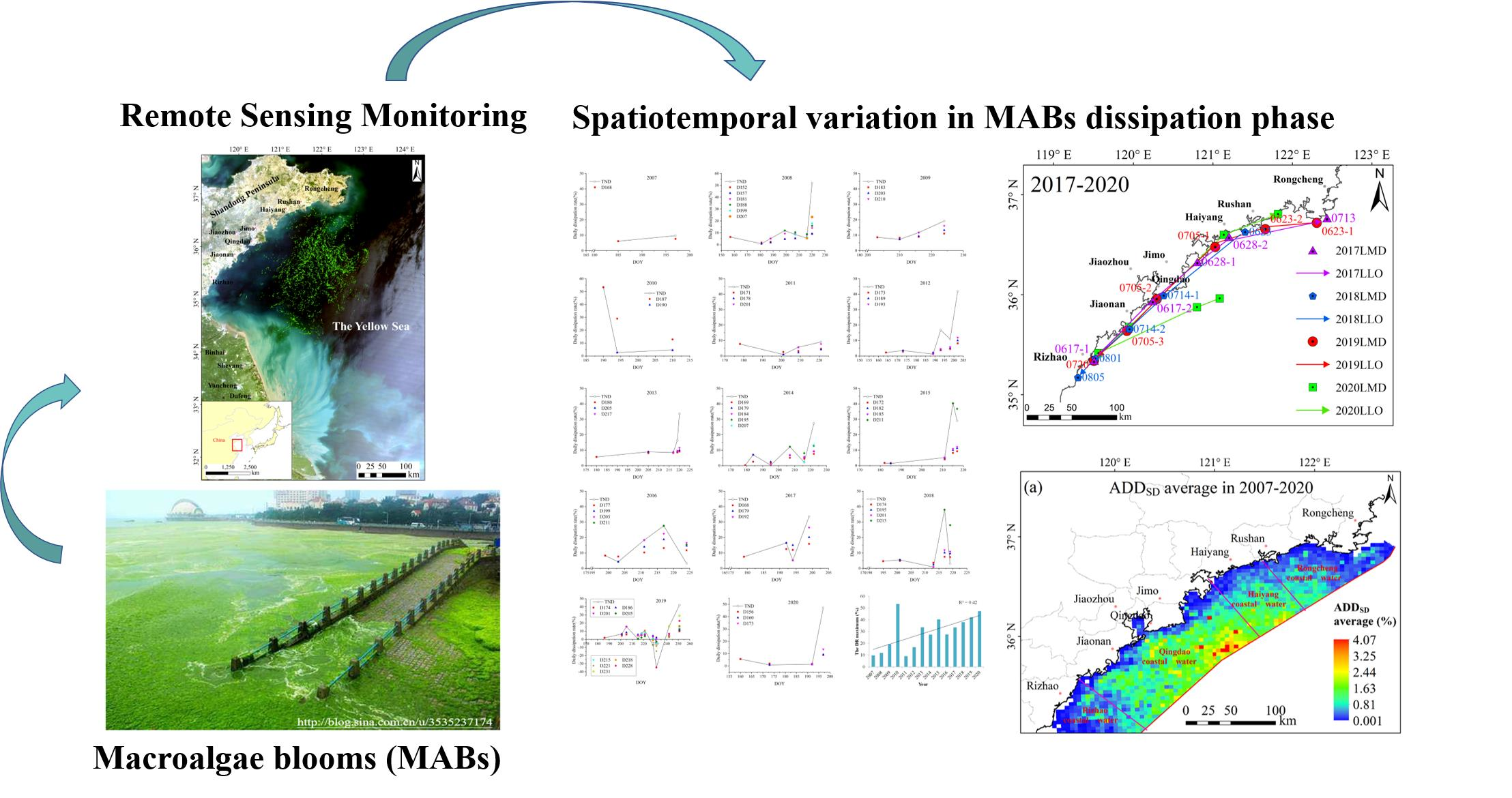
Monitoring the Dissipation of the Floating Green Macroalgae Blooms in the Yellow Sea (2007–2020) on the Basis of Satellite Remote Sensing


 ,
,
Abstract
:
1. Introduction
2. Data and Methods
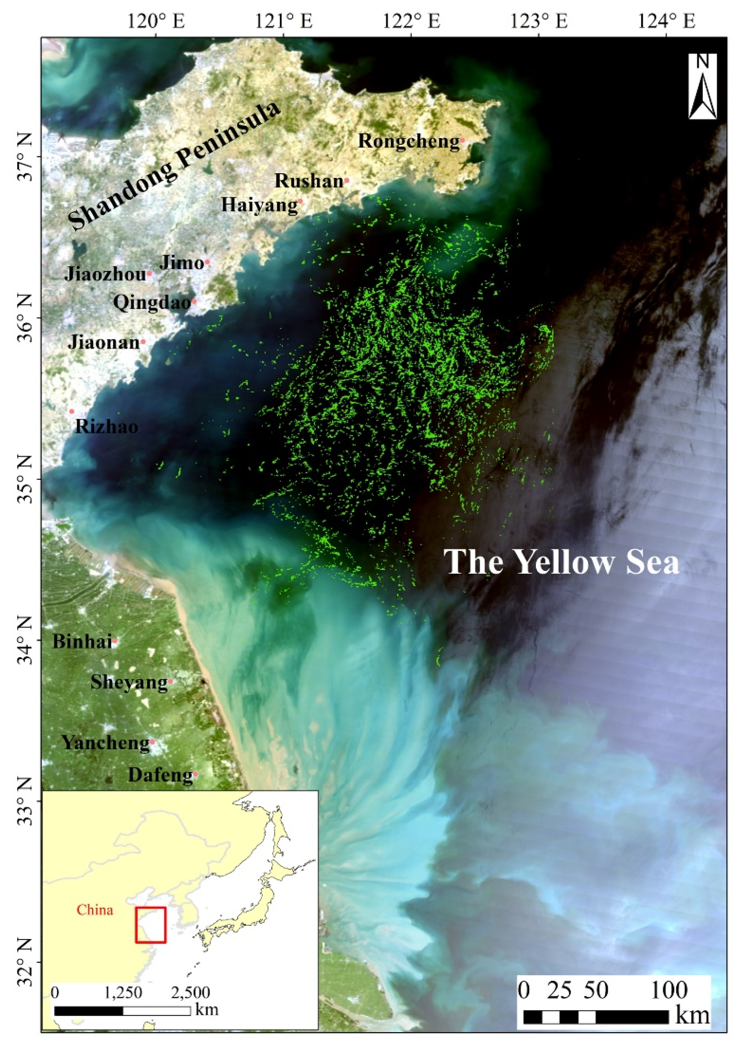
2.1. Study Area
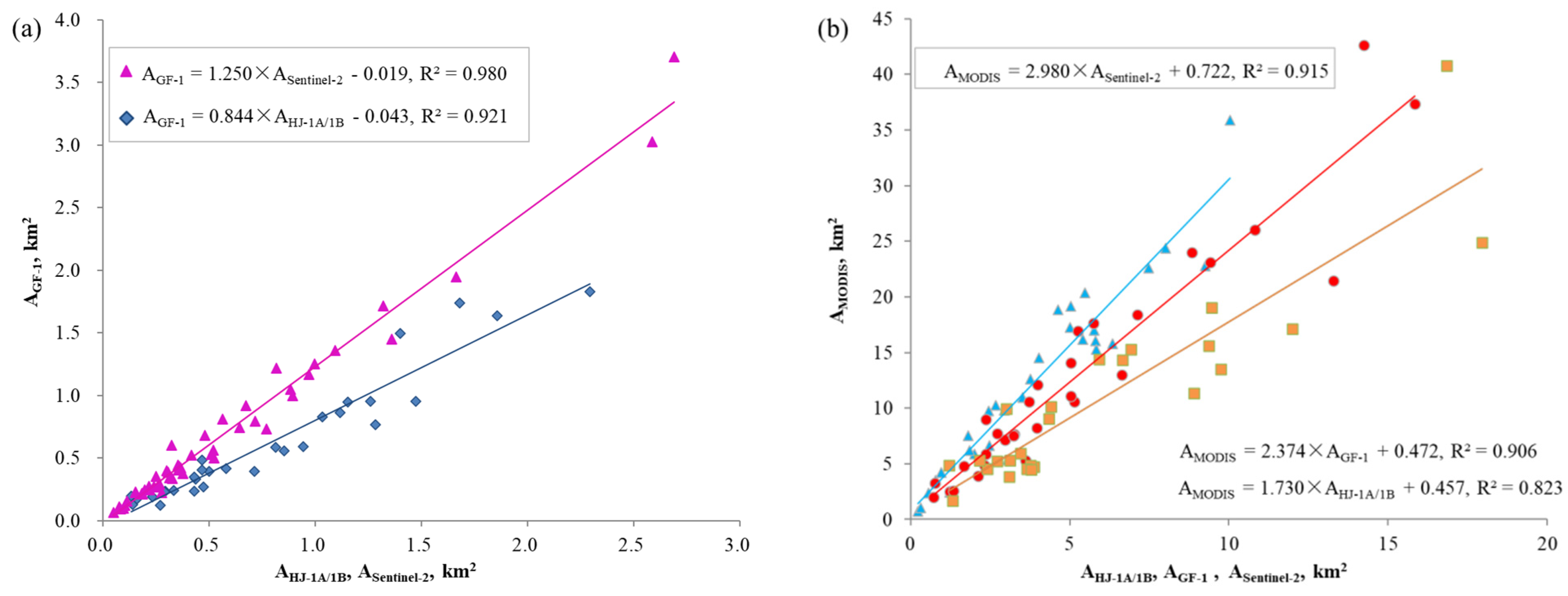
2.2. Remote Sensing Images, Data Processing, and MABs Area Statistics
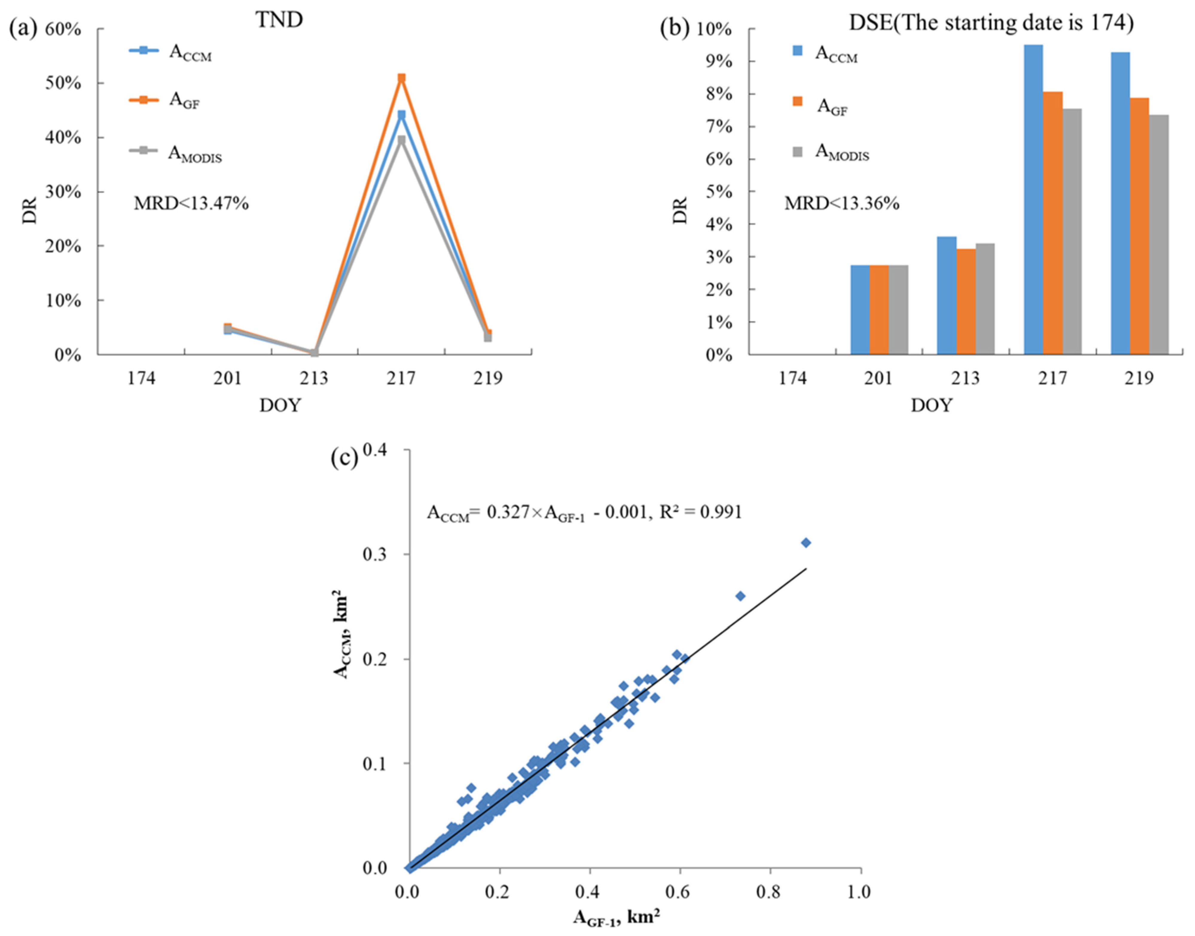
2.3. Calculation and Analysis of Macroalgae Daily Dissipation Rate
2.4. Analysis of the Spatiotemporal Variation in MABs Dissipation
3. Results
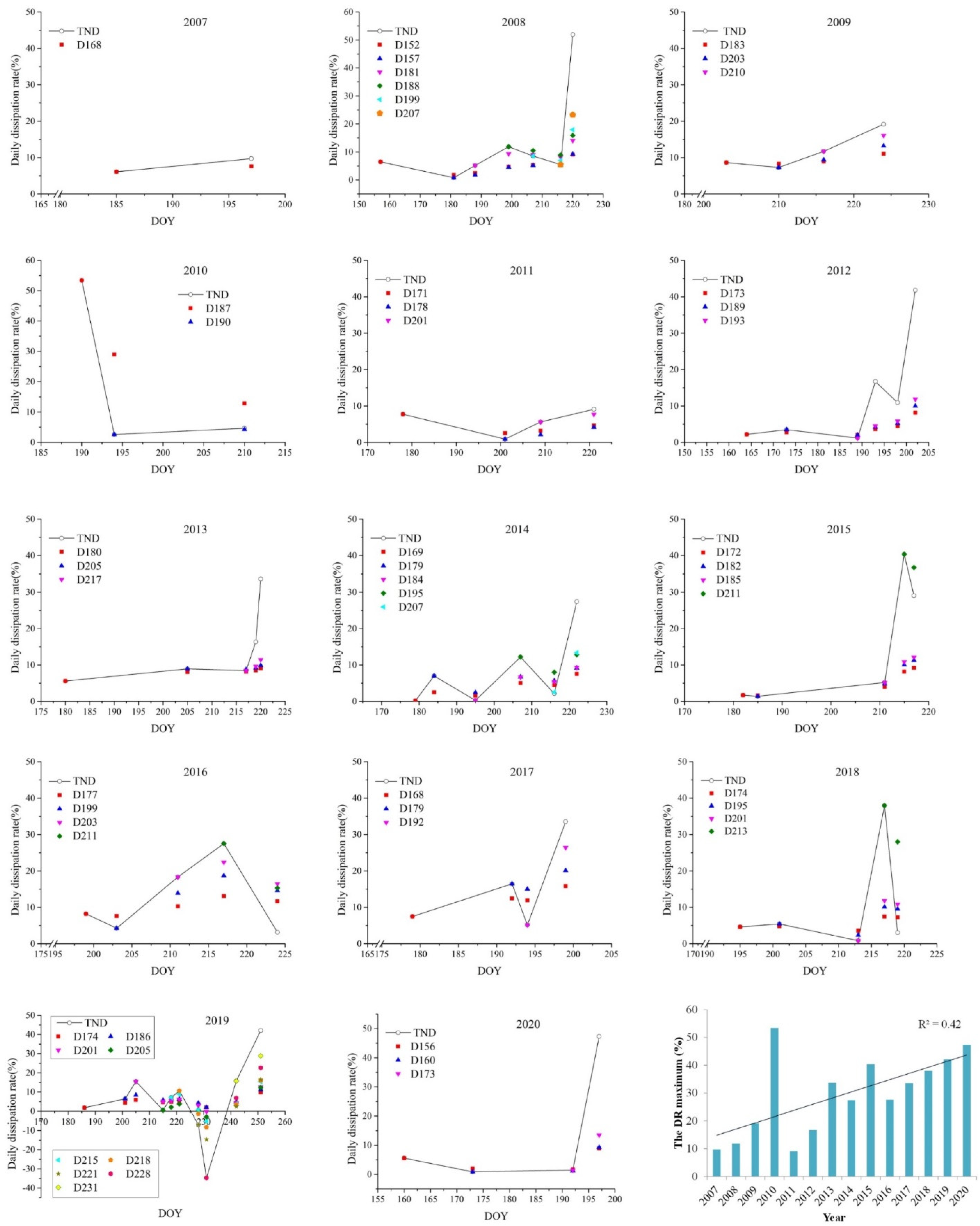
3.1. Variation in the Macroalgae Daily Dissipation Rate
- (1)
- A general decreasing trend and a maximum value of DR in the early stage of the dissipation phase, such as in 2010;
- (2)
- No obvious variation, such as in 2007 and 2011;
- (3)
- A general increasing trend and a maximum value of DR in the late stage of the dissipation phase, such as in 2009, 2013, 2014, 2017, 2019 and 2020;
- (4)
- A trend of TND decreasing at first, then increasing, and decreasing again, such as in 2008, 2012, 2016 and 2018;
- (5)
- A trend of TND increasing at first, then decreasing, such as in 2015.
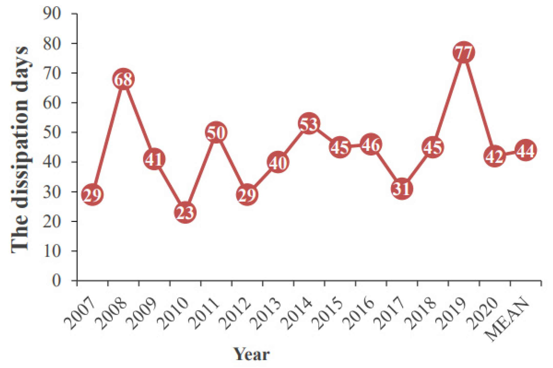
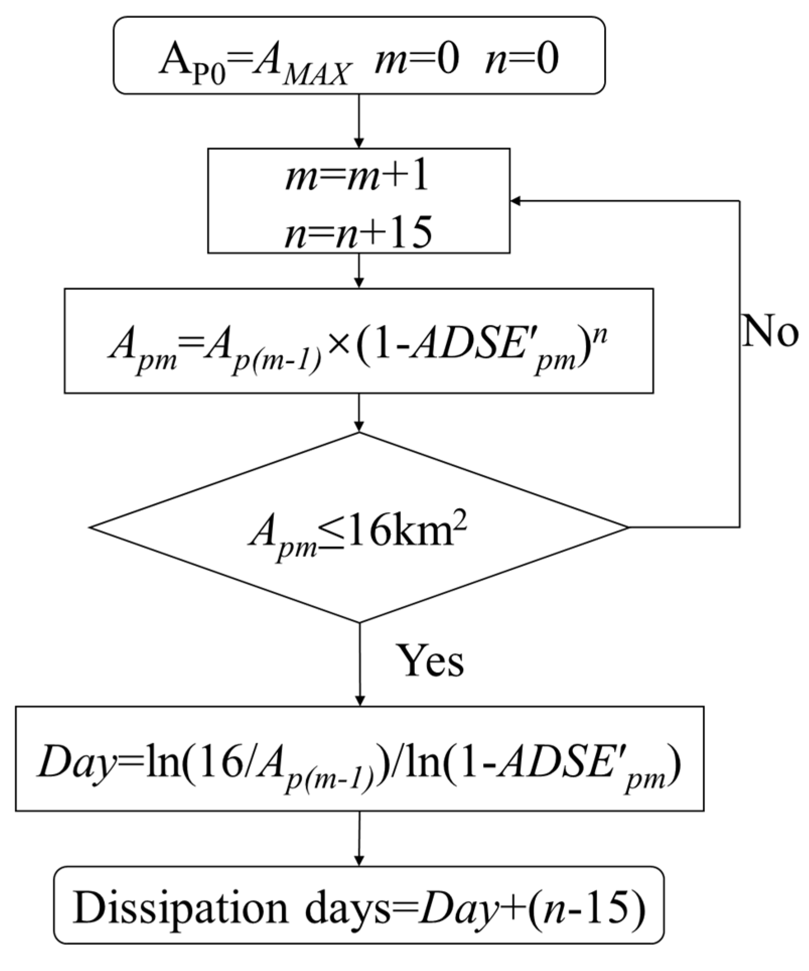
3.2. The Application of DR Variation: A Simple Method of Estimating Macroalgae Dissipation Days
- (1)
- The dissipation phase of MABs was divided into four stages (P1–P4) according to the annual dissipation days (Figure 7). P1–P4 was within 15 days after AMAX, 16–30 days, 31–45 days, and 46–60 days, respectively.
- (2)
- The DSE mean was calculated for each stage that described above from 2007 to 2017, denoted as DSE′, and the annual mean of DSE′, denoted as ADSE′ was also calculated. Note that the stage of the year was not included in the calculation if there were no images in that stage.
- (3)
- The dissipation days for these three years were estimated based on AMAX for 2018, 2019, and 2020 and ADSE′ of each stage. The detailed process is shown in Figure 8.
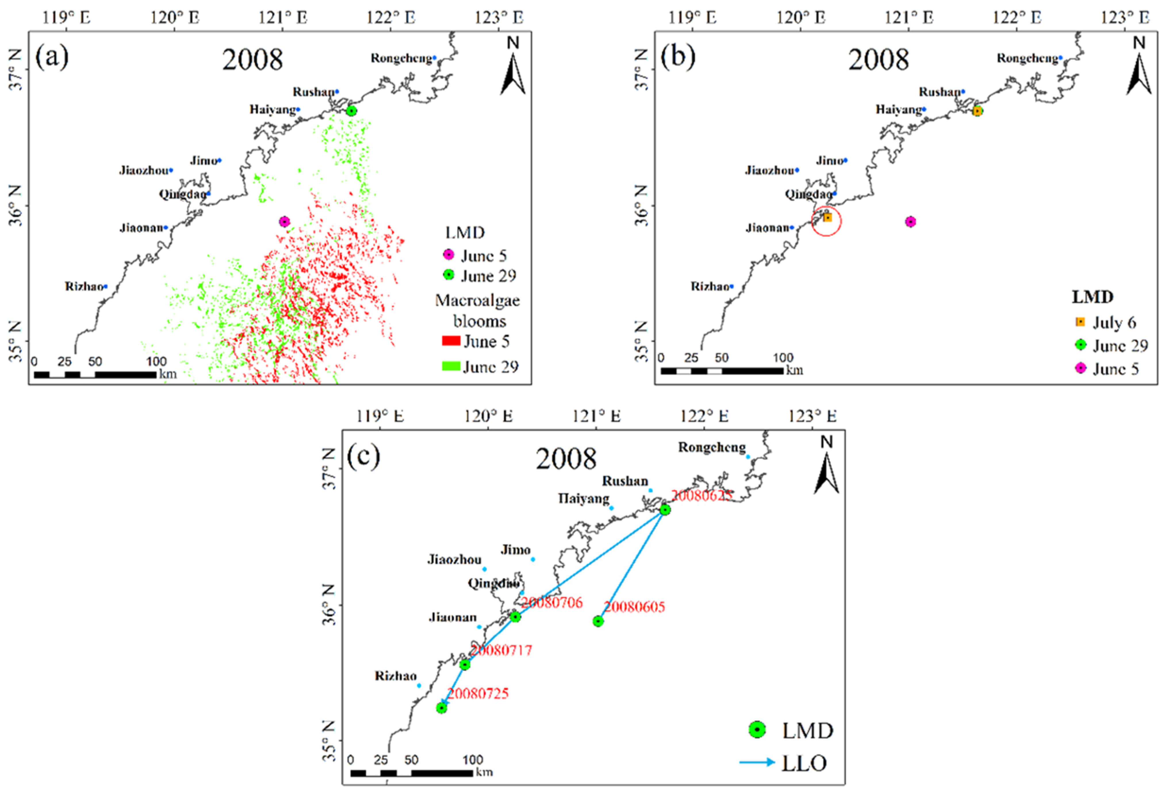
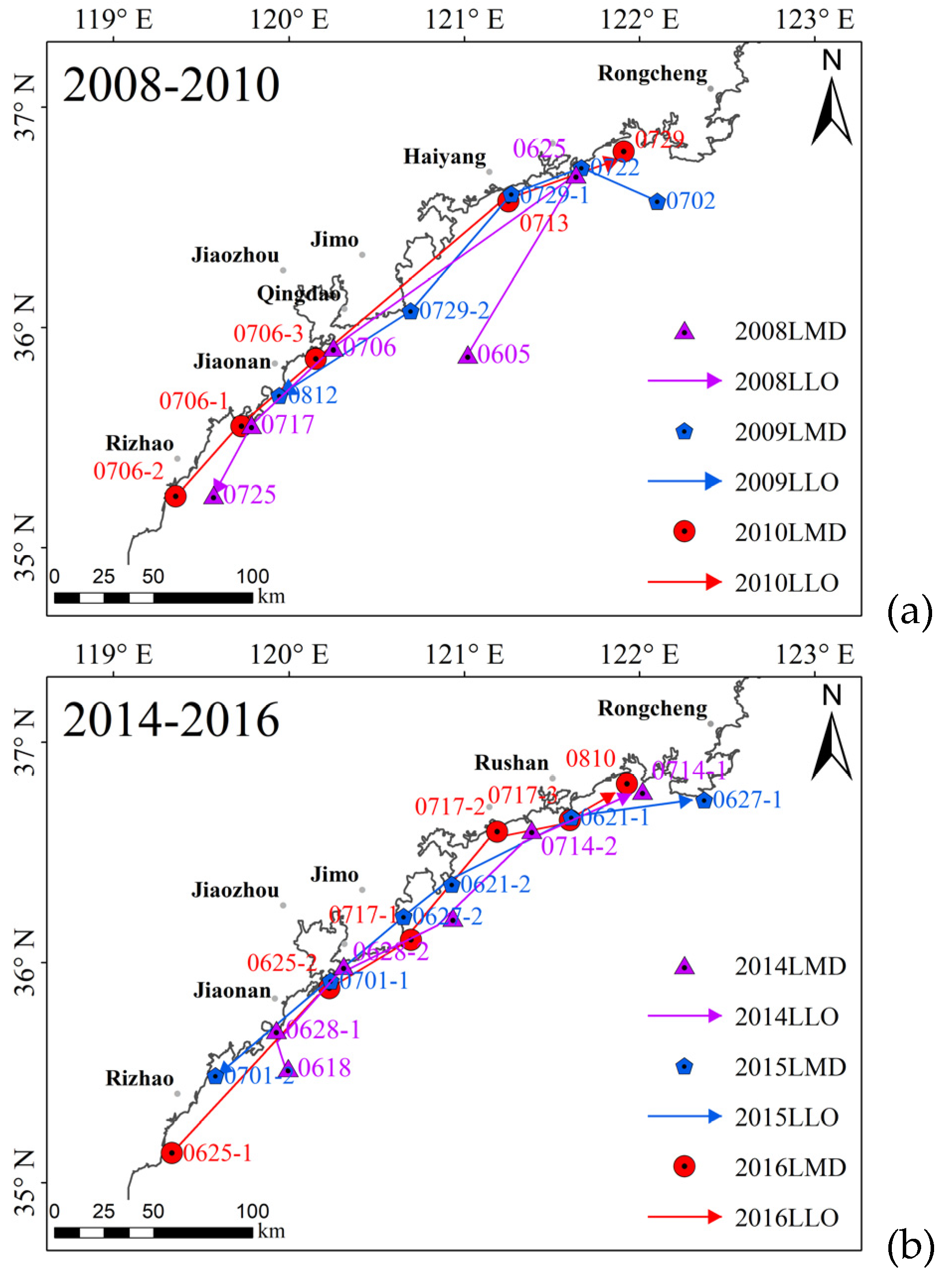
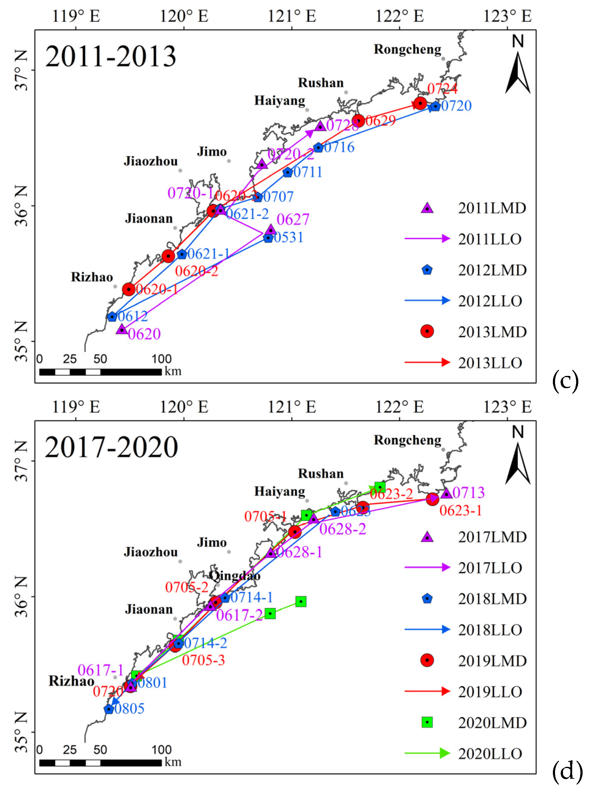
3.3. The LLO Variation in MABs Dissipation Phase from 2007 to 2020
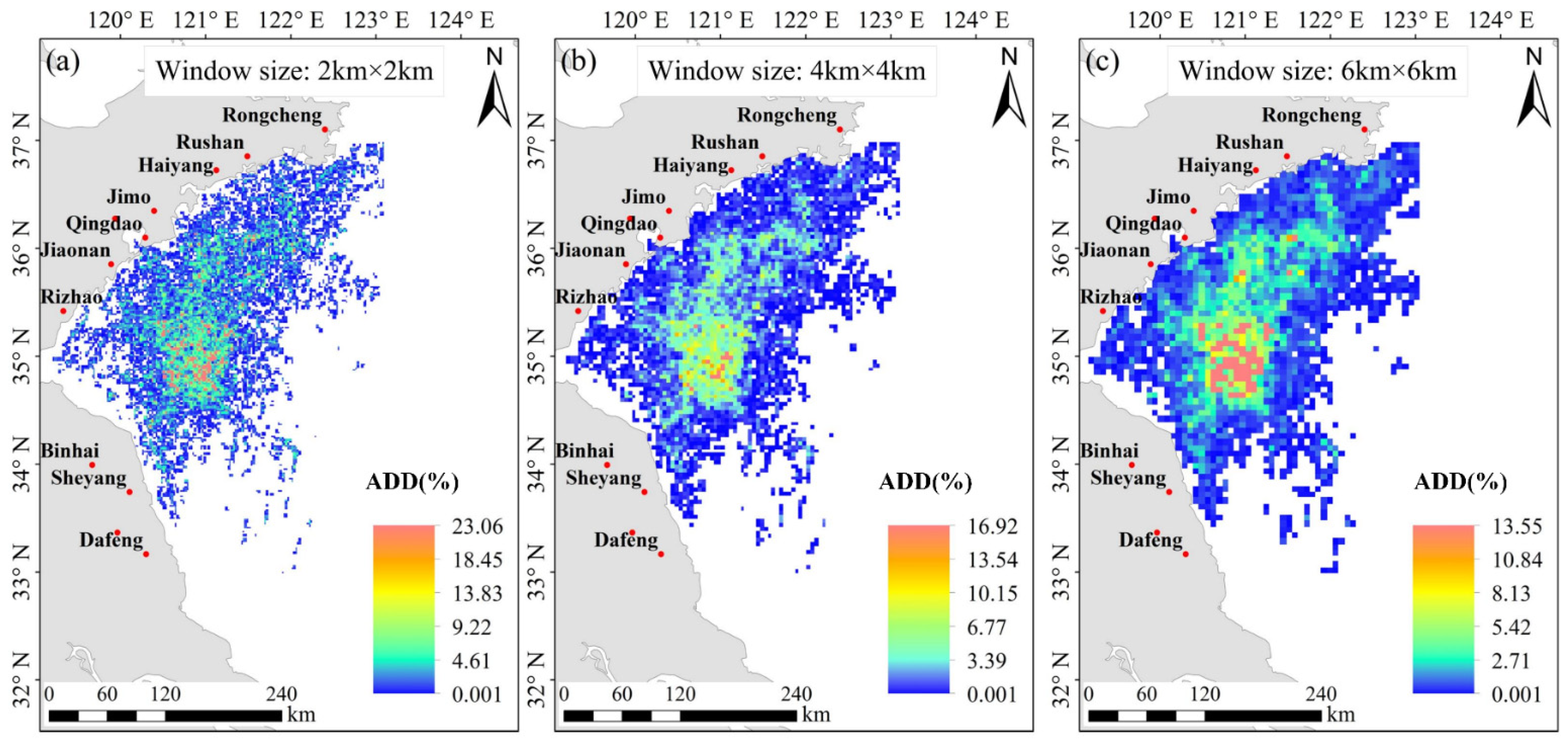
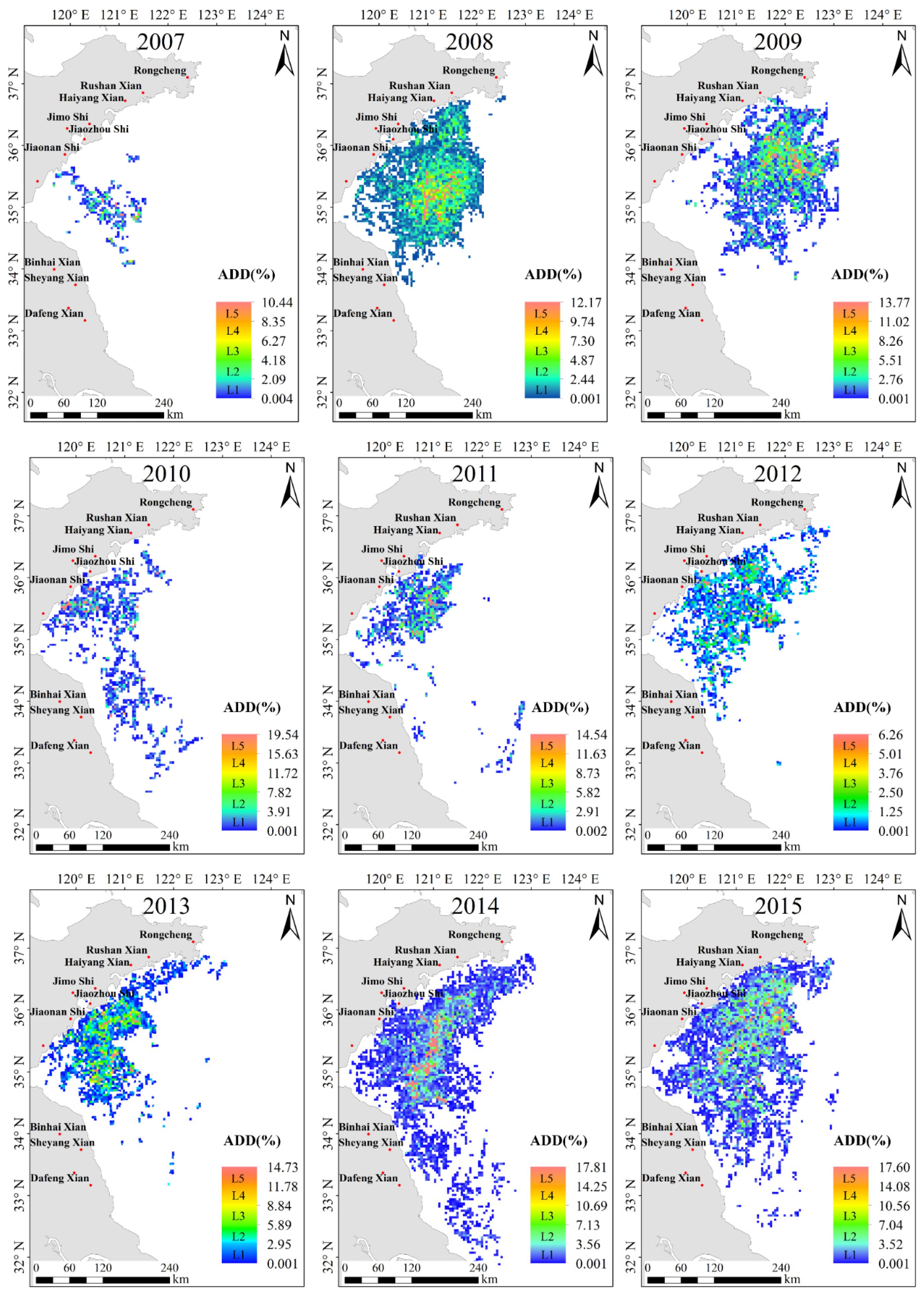
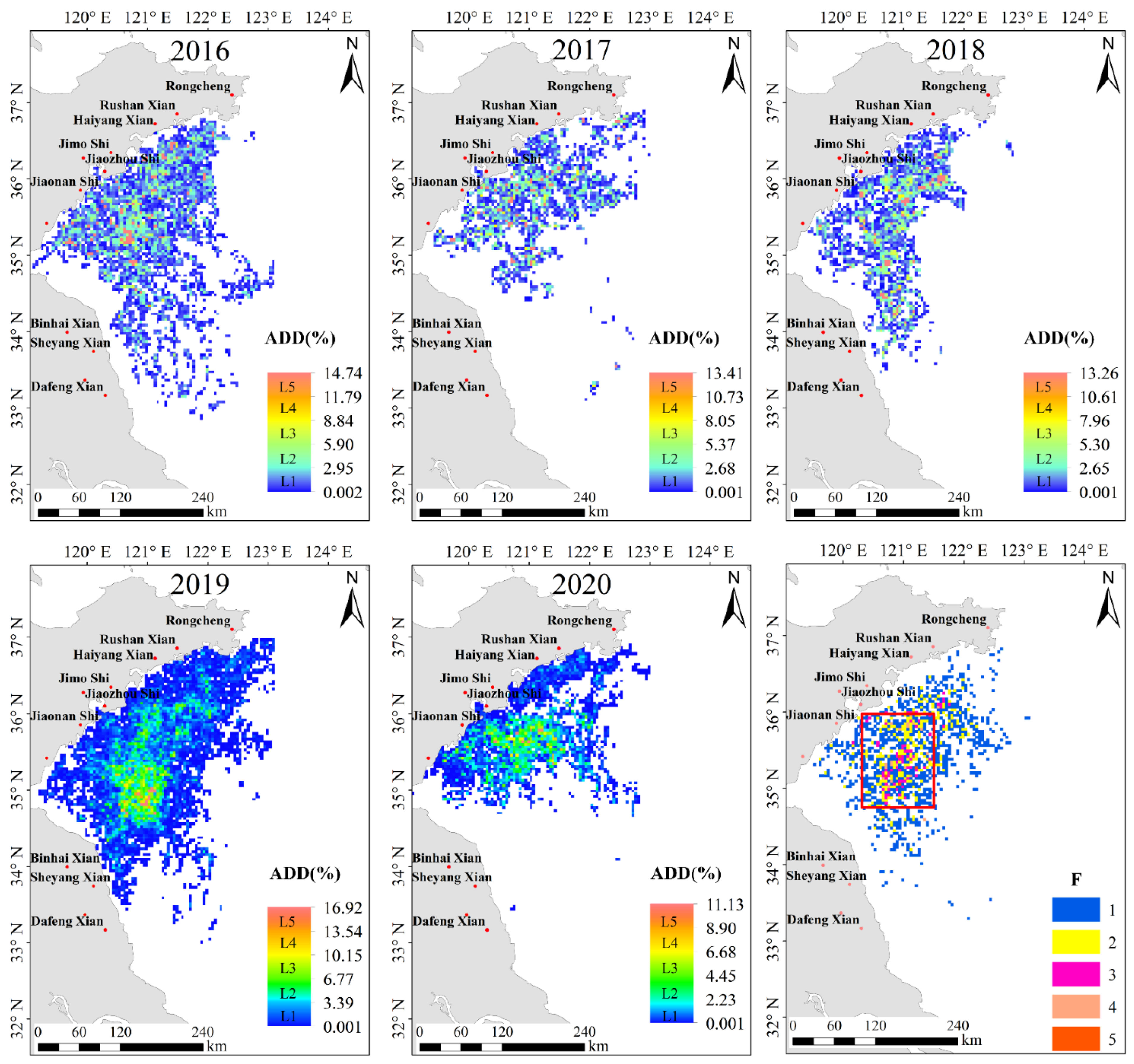
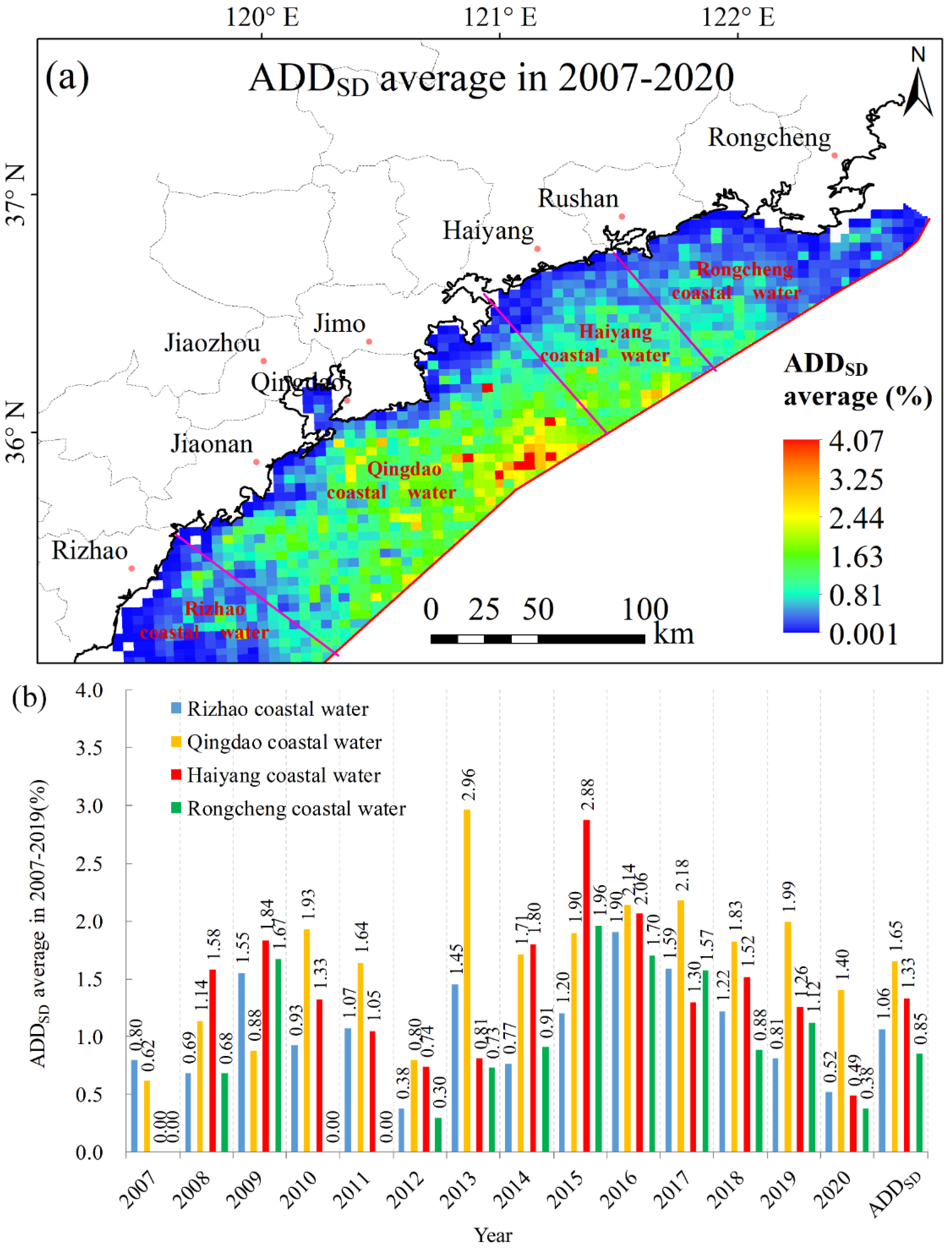
3.4. The Annual Distribution Density (ADD) Variation of MABs in the Dissipation Phase
4. Discussion
5. Conclusions
Author Contributions
Funding
Institutional Review Board Statement
Informed Consent Statement
Data Availability Statement
Acknowledgments
Conflicts of Interest
References
- Morand, P.; Merceron, M. Macroalgal Population and Sustainability. J. Coast. Res. 2005, 21, 1009–1020. [Google Scholar] [CrossRef]
- Smetacek, V.; Zingone, A. Green and golden seaweed tides on the rise. Nature 2013, 504, 84–88. [Google Scholar] [CrossRef] [Green Version]
- Wang, M.; Hu, C.; Barnes, B.B.; Mitchum, G.; Lapointe, B.; Montoya, J.P. The great Atlantic Sargassum belt. Science 2019, 365, 83–87. [Google Scholar] [CrossRef]
- Ye, N.H.; Zhang, X.W.; Mao, Y.Z.; Liang, C.W.; Xu, D.; Zou, J.; Zhuang, Z.M.; Wang, Q.Y. ‘Green tides’ are overwhelming the coastline of our blue planet: Taking the world’s largest example. Ecol. Res. 2011, 26, 477–485. [Google Scholar] [CrossRef]
- Song, X.L.; Huang, R.; Yuan, K.L.; Zhao, Y.H.; Wen, R.B.; Zhang, H.L. Characteristics of the green tide disaster of east Shandong Peninsula offshore. Mar. Environ. Sci. 2015, 34, 391–395. [Google Scholar] [CrossRef]
- Zhou, M.J.; Liu, D.Y.; Anderson, D.M.; Valiela, I. Introduction to the Special Issue on green tides in the Yellow Sea. Estuar. Coast. Shelf Sci. 2015, 163, 3–8. [Google Scholar] [CrossRef] [Green Version]
- Hu, C.M. A novel ocean color index to detect floating algae in the global oceans. Remote Sens. Environ. 2009, 113, 2118–2129. [Google Scholar] [CrossRef]
- Shi, W.; Wang, M.H. Green macroalgae blooms in the Yellow Sea during the spring and summer of 2008. J. Geophys. Res. Ocean. 2009, 114, C12010. [Google Scholar] [CrossRef] [Green Version]
- Xing, Q.G.; Hu, C.M. Mapping macroalgal blooms in the Yellow Sea and East China Sea using HJ-1 and Landsat data: Application of a virtual baseline reflectance height technique. Remote Sens. Environ. 2016, 178, 113–126. [Google Scholar] [CrossRef]
- Li, L.; Zheng, X.; Wei, Z.; Zou, J.; Xing, Q. A Spectral-Mixing Model for Estimating Sub-Pixel Coverage of Sea-Surface Floating Macroalgae. Atmos. Ocean 2018, 56, 296–302. [Google Scholar] [CrossRef]
- Qi, L.; Hu, C.M.; Xing, Q.G.; Shang, S.L. Long-term trend of Ulva prolifera blooms in the western Yellow Sea. Harmful Algae 2016, 58, 35–44. [Google Scholar] [CrossRef]
- Xing, Q.G.; Zheng, X.Y.; Shi, P.; Hao, J.J.; Yu, D.F.; Liang, S.Z.; Liu, D.Y.; Zhang, Y.Z. Monitoring “Green Tide” in the Yellow Sea and the East China Sea Using Multi-Temporal and Multi-Source Remote Sensing Images. Spectrosc. Spectr. Anal. 2011, 31, 1644–1647. [Google Scholar] [CrossRef]
- Hu, C.; Li, D.; Chen, C.; Ge, J.; Muller-Karger, F.E.; Liu, J.; Yu, F.; He, M.-X. On the recurrent Ulva prolifera blooms in the Yellow Sea and East China Sea. J. Geophys. Res. Oceans 2010, 115. [Google Scholar] [CrossRef] [Green Version]
- Xing, Q.; An, D.; Zheng, X.; Wei, Z.; Chen, J. Monitoring seaweed aquaculture in the Yellow Sea with multiple sensors for managing the disaster of macroalgal blooms. Remote Sens. Environ. 2019, 231, 111279. [Google Scholar] [CrossRef]
- Cao, Y.Z.; Wu, Y.C.; Fang, Z.X.; Cui, X.J.; Liang, J.F.; Song, X. Spatiotemporal Patterns and Morphological Characteristics of Ulva prolifera Distribution in the Yellow Sea, China in 2016–2018. Remote Sens. 2019, 11, 445. [Google Scholar] [CrossRef] [Green Version]
- Min, S.H.; Oh, H.J.; Hwang, J.D.; Suh, Y.S.; Kim, W. Tracking the Movement and Distribution of Green Tides on the Yellow Sea in 2015 Based on GOCI and Landsat Images. Korean J. Remote Sens. 2017, 33, 97–109. [Google Scholar] [CrossRef] [Green Version]
- Hu, S.; Yang, H.; Zhang, J.H.; Chen, C.S.; He, P.M. Small-scale early aggregation of green tide macroalgae observed on the Subei Bank, Yellow Sea. Mar. Pollut. Bull. 2014, 81, 166–173. [Google Scholar] [CrossRef] [PubMed]
- Son, Y.B.; Choi, B.J.; Kim, Y.H.; Park, Y.G. Tracing floating green algae blooms in the Yellow Sea and the East China Sea using GOCI satellite data and Lagrangian transport simulations. Remote Sens. Environ. 2015, 156, 21–33. [Google Scholar] [CrossRef]
- Xu, Q.; Zhang, H.Y.; Ju, L.; Chen, M.X. Interannual variability of Ulva prolifera blooms in the Yellow Sea. Int. J. Remote Sens. 2014, 35, 4099–4113. [Google Scholar] [CrossRef]
- Fan, S.; Fu, M.; Wang, Z.; Zhang, X.; Song, W.; Li, Y.; Liu, G.; Shi, X.; Wang, X.; Zhu, M. Temporal variation of green macroalgal assemblage on Porphyra aquaculture rafts in the Subei Shoal, China. Estuar. Coast. Shelf Sci. 2015, 163, 23–28. [Google Scholar] [CrossRef]
- Huo, Y.; Han, H.; Shi, H.; Wu, H.; Zhang, J.; Yu, K.; Xu, R.; Liu, C.; Zhang, Z.; Liu, K. Changes to the biomass and species composition of Ulva sp. on Porphyra aquaculture rafts, along the coastal radial sandbank of the Southern Yellow Sea. Mar. Pollut. Bull. 2015, 93, 210–216. [Google Scholar] [CrossRef]
- Liu, D.; Keesing, J.K.; Xing, Q.; Ping, S. World’s largest macroalgal bloom caused by expansion of seaweed aquaculture in China. Mar. Pollut. Bull. 2009, 58, 888–895. [Google Scholar] [CrossRef]
- Liu, X.; Li, Y.; Wang, Z.; Zhang, Q.; Cai, X. Cruise observation of Ulva prolifera bloom in the southern Yellow Sea, China. Estuar. Coast. Shelf Sci. 2015, 163, 17–22. [Google Scholar] [CrossRef]
- Zhang, J.; Huo, Y.; Wu, H.; Yu, K.; Kim, J.K.; Yarish, C.; Qin, Y.; Liu, C.; Ren, X.; He, P. The origin of the Ulva macroalgal blooms in the Yellow Sea in 2013. Mar. Pollut. Bull. 2014, 89, 276–283. [Google Scholar] [CrossRef]
- Zheng, X.Y.; Xing, Q.G.; Li, L.I.; Shi, P. Numerical simulation of the 2008 green tide in the Yellow Sea. Mar. Sci. 2011, 35, 82–87. [Google Scholar]
- Huo, Y.; Han, H.; Hua, L.; Wei, Z.; Yu, K.; Shi, H.; Kim, J.K.; Yarish, C.; He, P. Tracing the origin of green macroalgal blooms based on the large scale spatio-temporal distribution of Ulva microscopic propagules and settled mature Ulva vegetative thalli in coastal regions of the Yellow Sea, China. Harmful Algae 2016, 59, 91–99. [Google Scholar] [CrossRef] [PubMed]
- Song, W.; Li, Y.; Fang, S.; Wang, Z.; Xiao, J.; Li, R.; Fu, M.; Zhu, M.; Zhang, X. Temporal and spatial distributions of green algae micro-propagules in the coastal waters of the Subei Shoal, China. Estuar. Coast. Shelf Sci. 2015, 163, 29–35. [Google Scholar] [CrossRef]
- Xing, Q.; Wu, L.; Tian, L.; Cui, T.; Wu, M. Remote sensing of early-stage green tide in the Yellow Sea for floating-macroalgae collecting campaign. Mar. Pollut. Bull. 2018, 133, 150–156. [Google Scholar] [CrossRef] [PubMed]
- Wang, Z.; Xiao, J.; Fan, S.; Li, Y.; Liu, X.; Liu, D. Who made the world’s largest green tide in China?—An integrated study on the initiation and early development of the green tide in Yellow Sea. Limnol. Oceanogr. 2015, 60, 1105–1117. [Google Scholar] [CrossRef]
- Wei, Q.; Wang, B.; Yao, Q.; Fu, M.; Sun, J.; Xu, B.; Yu, Z. Hydro-biogeochemical processes and their implications for Ulva prolifera blooms and expansion in the world’s largest green tide occurrence region (Yellow Sea, China). Sci. Total Environ. 2018, 645, 257–266. [Google Scholar] [CrossRef]
- Xu, Q.; Zhang, H.; Cheng, Y.; Zhang, S.; Wei, Z. Monitoring and Tracking the Green Tide in the Yellow Sea With Satellite Imagery and Trajectory Model. IEEE J. Sel. Top. Appl. Earth Obs. Remote Sens. 2017, 9, 5172–5181. [Google Scholar] [CrossRef]
- Xing, Q.G.; Hu, C.M.; Tang, D.L.; Tian, L.Q.; Tang, S.L.; Wang, X.H.; Lou, M.J.; Gao, X.L. World’s Largest Macroalgal Blooms Altered Phytoplankton Biomass in Summer in the Yellow Sea: Satellite Observations. Remote Sens. 2015, 7, 12297–12313. [Google Scholar] [CrossRef] [Green Version]
- Li, L.; Xing, Q.; Li, X.; Yu, D.; Zhang, J.; Zou, J. Assessment of the Impacts From the World’s Largest Floating Macroalgae Blooms on the Water Clarity at the West Yellow Sea Using MODIS Data (2002–2016). IEEE J. Sel. Top. Appl. Earth Obs. Remote Sens. 2018, 11, 1397–1402. [Google Scholar] [CrossRef]
- Wu, X.Q.; Xu, K.D.; Yu, Z.S.; Yu, T.T.; Lei, Y.L. Standing crop and spatial distribution of meiofauna in Yellow Sea at late stage of Enteromorpha prolifera bloom in 2008. Chin. J. Appl. Ecol. 2010, 21, 2140–2147. [Google Scholar] [CrossRef]
- Tq, A.; Xz, A.; Yh, A.; Yi, Z.A.; Chen, G.A.; Ch, A.; Xta, B.; Ying, W. Ecological effects of Ulva prolifera green tide on bacterial community structure in Qingdao offshore environment. Chemosphere 2020, 244, 125477. [Google Scholar] [CrossRef]
- Wang, X.H.; Li, L.; Bao, X.; Zhao, L.D. Economic Cost of an Algae Bloom Cleanup in China’s 2008 Olympic Sailing Venue. Eos Trans. Am. Geophys. Union 2013, 90, 238–239. [Google Scholar] [CrossRef]
- Cui, T.W.; Liang, X.J.; Gong, J.L.; Tong, C.; Xiao, Y.F.; Liu, R.J.; Zhang, X.; Zhang, J. Assessing and refining the satellite-derived massive green macro-algal coverage in the Yellow Sea with high resolution images. ISPRS J. Photogramm. Remote Sens. 2018, 144, 315–324. [Google Scholar] [CrossRef]
- Guo, W.; Zhao, L.; Li, X.M. The interannual variation of Green Tide in the Yellow Sea. Haiyang Xuebao 2016, 38, 36–45. [Google Scholar] [CrossRef]
- Xiao, Y.F.; Zhang, J.; Cui, T.W. High-precision extraction of nearshore green tides using satellite remote sensing data of the Yellow Sea, China. Int. J. Remote Sens. 2017, 38, 1626–1641. [Google Scholar] [CrossRef]
- Hu, L.B.; Zeng, K.; Hu, C.M.; He, M.X. On the remote estimation of Ulva prolifera areal coverage and biomass. Remote Sens. Environ. 2019, 223, 194–207. [Google Scholar] [CrossRef]
- Jian, L.U.; Zhang, Q.L.; An-Chun, L.I. The influence of Subei coastal current on the outbreak and drift of Enteromorpha prolifera. Mar. Sci. 2014, 10, 83–89. [Google Scholar] [CrossRef]
- Lee, J.H.; Pang, I.-C.; Moon, I.-J.; Ryu, J.-H. On physical factors that controlled the massive green tide occurrence along the southern coast of the Shandong Peninsula in 2008: A numerical study using a particle-tracking experiment. J. Geophys. Res. Oceans 2011, 116. [Google Scholar] [CrossRef] [Green Version]
- Zhang, S.P.; Liu, Y.C.; Zhang, G.Q.; Lei, G. Analysis on the Hydro-Moteorological Conditions from Remote Sensing Data for the 2008 Algal Blooming in the Yellow Sea. Period. Ocean Univ. China 2009, 39, 870–876. [Google Scholar] [CrossRef]
- Wang, Z.; Fu, M.; Jie, X.; Zhang, X.; Wei, S. Progress on the study of the Yellow Sea green tides caused by Ulva prolifera. Haiyang Xuebao 2018, 40, 1–13. [Google Scholar] [CrossRef]


| Year | DSE’(%) | |||
|---|---|---|---|---|
| P1 | P2 | P3 | P4 | |
| 2007 | -- | 7.61 | -- | -- |
| 2008 | 6.48 | 0.78 | 5.19 | 9.09 |
| 2009 | -- | 8.30 | 13.24 | -- |
| 2010 | 28.99 | 4.64 | -- | -- |
| 2011 | 7.72 | 0.88 | 5.60 | 9.08 |
| 2012 | 2.19 | 3.47 | 4.18 | 23.47 |
| 2013 | 5.57 | -- | 8.92 | 11.46 |
| 2014 | 0.17 | 1.56 | 12.18 | 12.80 |
| 2015 | 1.64 | -- | 11.26 | -- |
| 2016 | -- | 7.62 | 18.70 | 3.16 |
| 2017 | 7.50 | 15.03 | 33.53 | -- |
| ADSE’ | 7.53 | 5.54 | 12.53 | 11.51 |
| Year | AMAX (km2) | MAB Dissipation Days | Relative Error (%) | |||
|---|---|---|---|---|---|---|
| n | Day | Estimation Days | Actual Days | |||
| 2018 | 1493.70 | 45 | 5 | 50 | 45 | 11.11 |
| 2019 | 3284.94 | 45 | 11 | 56 | 77 | 27.27 |
| 2020 | 640.56 | 30 | 13 | 43 | 42 | 2.38 |
Publisher’s Note: MDPI stays neutral with regard to jurisdictional claims in published maps and institutional affiliations. |
© 2021 by the authors. Licensee MDPI, Basel, Switzerland. This article is an open access article distributed under the terms and conditions of the Creative Commons Attribution (CC BY) license (https://creativecommons.org/licenses/by/4.0/).
Share and Cite
An, D.; Yu, D.; Zheng, X.; Zhou, Y.; Meng, L.; Xing, Q. Monitoring the Dissipation of the Floating Green Macroalgae Blooms in the Yellow Sea (2007–2020) on the Basis of Satellite Remote Sensing. Remote Sens. 2021, 13, 3811. https://doi.org/10.3390/rs13193811
An D, Yu D, Zheng X, Zhou Y, Meng L, Xing Q. Monitoring the Dissipation of the Floating Green Macroalgae Blooms in the Yellow Sea (2007–2020) on the Basis of Satellite Remote Sensing. Remote Sensing. 2021; 13(19):3811. https://doi.org/10.3390/rs13193811
Chicago/Turabian StyleAn, Deyu, Dingfeng Yu, Xiangyang Zheng, Yan Zhou, Ling Meng, and Qianguo Xing. 2021. "Monitoring the Dissipation of the Floating Green Macroalgae Blooms in the Yellow Sea (2007–2020) on the Basis of Satellite Remote Sensing" Remote Sensing 13, no. 19: 3811. https://doi.org/10.3390/rs13193811