Estimation of Northern Hardwood Forest Inventory Attributes Using UAV Laser Scanning (ULS): Transferability of Laser Scanning Methods and Comparison of Automated Approaches at the Tree- and Stand-Level

Abstract

UAV laser scanning (ULS) has the potential to support forest operations since it provides high-density data with flexible operational conditions. This study examined the use of ULS systems to estimate several tree attributes from an uneven-aged northern hardwood stand. We investigated: (1) the transferability of raster-based and bottom-up point cloud-based individual tree detection (ITD) algorithms to ULS data; and (2) automated approaches to the retrieval of tree-level (i.e., height, crown diameter (CD), DBH) and stand-level (i.e., tree count, basal area (BA), DBH-distribution) forest inventory attributes. These objectives were studied under leaf-on and leaf-off canopy conditions. Results achieved from ULS data were cross-compared with ALS and TLS to better understand the potential and challenges faced by different laser scanning systems and methodological approaches in hardwood forest environments. The best results that characterized individual trees from ULS data were achieved under leaf-off conditions using a point cloud-based bottom-up ITD. The latter outperformed the raster-based ITD, improving the accuracy of tree detection (from 50% to 71%), crown delineation (from R² = 0.29 to R² = 0.61), and prediction of tree DBH (from R² = 0.36 to R² = 0.67), when compared with values that were estimated from reference TLS data. Major improvements were observed for the detection of trees in the lower canopy layer (from 9% with raster-based ITD to 51% with point cloud-based ITD) and in the intermediate canopy layer (from 24% with raster-based ITD to 59% with point cloud-based ITD). Under leaf-on conditions, LiDAR data from aerial systems include substantial signal occlusion incurred by the upper canopy. Under these conditions, the raster-based ITD was unable to detect low-level canopy trees (from 5% to 15% of trees detected from lower and intermediate canopy layers, respectively), resulting in a tree detection rate of about 40% for both ULS and ALS data. The cylinder-fitting method used to estimate tree DBH under leaf-off conditions did not meet inventory standards when compared to TLS DBH, resulting in RMSE = 7.4 cm, Bias = 3.1 cm, and R² = 0.75. Yet, it yielded more accurate estimates of the BA (+3.5%) and DBH-distribution of the stand than did allometric models −12.9%), when compared with in situ field measurements. Results suggest that the use of bottom-up ITD on high-density ULS data from leaf-off hardwood forest leads to promising results when estimating trees and stand attributes, which opens up new possibilities for supporting forest inventories and operations.

1. Introduction

Achieving sustainability in timber supply requires forest managers to evaluate the short- and long-term ecological and economic consequences of their silvicultural treatments based on the actual and predicted forest conditions. Forest planning processes over decades involve breaking down decision-making into three components: strategic (≈20 years), tactical (≈5 years), and operational (≈1 year) (see [1,2]). The operational level focuses on scheduling harvest crews on a monthly or weekly basis and on optimizing wood flow. Accurate and up-to-date knowledge on the distribution of tree size, species, health, and growth of forest stands are essential for the planning and monitoring of forest operations. Tree-by-tree measurements are typically carried out in situ on forest sample plots and up-scaling approaches are used to assess forest resources over larger areas. However, the high labor and time costs of these conventional inventory techniques [3] currently lead to either the implementation being avoided all together or to sample size being reduced dramatically, thus limiting spatial and temporal resolution of field surveys and rendering them inadequate to provide high-resolution stand and tree characterization.

Limitations associated with current inventory practices are particularly acute for the management of uneven-aged forests, where objectives are usually consistent with close-to-nature silvicultural practices [4,5]. This leads to an increase in sophistication of silviculture regimes and is based on current stand and microsite conditions [6]. Instead of clearcutting or regular shelterwood systems, this approach often relies on long-term irregular shelterwood and individual tree selection regimes that require repeated interventions. This aims to regenerate the stand continuously and increase species richness while leaving some permanent forest cover to promote favorable forest development [7]. In this context, improving timber quality through better selection of trees to remove and a stronger focus on the conditions that are desired post-harvest are key management objectives. Improved inventory methods, therefore, are needed to support these complex interventions [8].

The past two decades have seen significant progress in the development of laser scanning techniques for improving forest inventories beyond photo-interpretation methods [9,10,11,12]. Airborne laser scanning (ALS) systems have become a dominant form of support for predicting forest biophysical/inventory attributes at the plot- and stand -levels [13]. Continuous advances in technological developments allow the acquisition of higher density ALS data (>12 points/m²), making it possible to derive individual tree attributes (see [14,15,16,17,18,19,20,21]). In this context, numerous algorithms have been developed for individual tree detection and delineation (ITD) from LiDAR point clouds (see [22,23,24] for reviews). ITD algorithms are generally based on three sequential steps involving tree detection, tree delineation, and tree attribute estimation [25]. The tree detection step can be raster-based, point cloud-based, or a combination of the two [22,25]. Raster-based ITD usually involves tree top detection (e.g., local maximum, image binarization, or template matching [16]) and crown delineation (e.g., valley-following, region-growing, or watershed segmentation [26,27]) from the canopy height model (CHM) to extract individual trees and further estimate their structural attributes (i.e., tree height and crown dimensions and predicted diameter at breast height (DBH), volume, or biomass, e.g., [28]). Point cloud-based ITD usually requires K-means clustering (e.g., [18,20,29,30,31,32]) or voxel-based tree segmentation techniques (i.e., [33,34]) to extract individual trees directly from the 3D point cloud and estimate their attributes through geometric modeling techniques (i.e., convex hull, alpha shape, super quadratic or Hough transform, e.g., [35,36,37,38,39]). So far, raster-based ITD is mostly used for ALS data processing [23] because it is computationally efficient over large forest areas and, unlike point cloud-based ITD, it is also more widely available and simpler to implement for the user.

However, the use of ITD approaches using ALS data remains operationally limited and is still under investigation [40]. This is mainly due to these approaches’ limited applicability to heterogeneous forest structures and the challenge that is associated with detecting understory trees (see benchmarks [41,42,43,44]). Crown of hardwood trees are also particularly difficult to detect for ITD algorithms, as a single tree can produce multiple crowns. ITD algorithms from terrestrial laser scanning (TLS) data are also available [45], but their adaptability and performance with respect to aerial LiDAR data is still unclear. The success of ITD depends on multiple factors, such as the density and the stand configuration [27,46,47,48], the point density of the LiDAR acquisition [49,50], the foliage condition [51,52,53], and the type of ITD algorithm that is applied (e.g., [30,42]). Research into ITD development is still actively needed to overcome the previously mentioned challenges and limitations.

With the recent accessibility of fully integrated compact LiDAR systems (i.e., laser scanner unit, GPS receivers, and inertial measurement unit (IMU)) and the continuous progress being made regarding unmanned aerial vehicles (UAVs) [54,55], UAV laser scanning systems (ULS) are becoming increasingly accessible for a wide range of applications [56], including forestry. The potential of UAVs for forestry lies in: (i) their flexible navigation systems that allow adapted flying patterns; (ii) their limited logistics and deployment permitting flights as needed in narrow window periods; and (iii) their ability to fly lower and slower than ALS or helicopters with an aerial perspective. In addition, ULS systems have certain advantages over ground-based data collection, for example: (i) they are not affected by the constraints of terrain access and the degradation of the Global Navigation Satellite System (GNSS) signals under the canopy [57]; (ii) the flexibility of their flying patterns facilitates multiple views of all points of a scene, which in turn reduces signal occlusion, an issue for all LiDAR systems; and (iii) their point density resolution can easily be adjusted during the flight configuration, permitting the collection of high (50 points/m² [58,59]), very-high (1500 points/m² [60]), to ultra-high (4000 points/m² [61]) density point clouds, thereby decreasing the boundaries between the ALS and TLS systems [57,62]. Most of all, the emergence of high-density ULS point clouds brings new opportunities to characterize forest resources at the tree-level.

ULS systems represent an interesting alternative to aerial surveys for small (up to 4 ha) to medium (4–400 ha) size areas. Such areas may be costly for an ALS data collection [63] or require too much time for full coverage by ground-based units [64]. More and more studies have demonstrated that ULS provides accurate data with good repeatability [58,65,66,67,68] and has great potential to support forest inventories (e.g., [57,66,67,68,69,70,71,72]). Transferability of ITD to ULS data is now actively being investigated (e.g., [73,74,75,76,77]). Despite encouraging results, most recent studies were conducted on softwood stands or on planted forests. There is still little scientific information regarding the potential of ULS systems on heterogeneous mixedwood or hardwood forests [59,78,79]. The structural complexity of these forest types, which pose additional challenges to the ITD algorithms, also increases the difficulty of validating results at the tree-level [49].

The main objective of this study was to investigate methodological approaches using ULS data to estimate forest inventory attributes from a naturally grown hardwood stand. This was accomplished by: (i) assessing the transferability of ITD algorithms that were developed for processing ALS and TLS data to ULS data that were collected under various canopy conditions (i.e., leaf-on and leaf-off); and (ii) comparing automated approaches for the retrieval of forest inventory attributes at the tree-level (i.e., height, crown diameter (CD), DBH) and at the stand-level (i.e., tree count, basal area (BA), DBH-distribution). For both sub-objectives, cross-comparisons between ALS, TLS, and ULS data were performed to provide a comprehensive understanding of the challenges facing various LiDAR data collection systems and processing algorithms. Results are expected to provide guidance in the use of ULS systems in supporting hardwood forest management.

2. Materials

2.1. Study Site

The study area (Figure 1) was located on a 25 ha stand in the McCoy Brook Forest, northeast of Edmundston (NB, Canada), about 320 m above sea level (47°27′01″N, 68°06′22″W). The area is located in the central uplands ecoregion in the Madawaska eco-district and belongs to the hardwood temperate zone [80]. The study site consisted of a 1 ha naturally grown hardwood stand with an uneven-aged structure. The last significant disturbance due to harvesting on this stand was about 100 years old. Sugar maple (Acer saccharum Marshall, 58%) is the dominant canopy tree species, with yellow birch (Betula alleghaniensis Britton, 16%), American beech (Fagus grandifolia Ehrhart, 11%), and red maple (Acer rubrum L., 6%) as co-dominant species. Suppressed understory trees are mainly juvenile balsam fir (Abies balsamea (L.) Miller, 9%).

2.2. Field Inventory

Traditional field measurements were conducted in summer 2017 in the study site of 1 ha for all 477 merchantable stems of the stand (DBH ≥ 9 cm). Each tree was marked and numbered in the field, and geo-referenced using Topcon GNSS Real Time Kinematic (RTK) equipment. DBH (at 1.3 m) was measured with a measuring tape and tree height using a Haglöf Vertex IV hypsometer equipped with a T3 transponder (Haglöf Sweden, AB, Långsele, Sweden). The mean and median height of trees on the stand were 16.1 m and 16.2 m, respectively. The mean and median DBH of trees on the stand were 20.1 cm and 24.1 cm, respectively. The structural complexity of the stand can be captured in the DBH-distribution (Figure 2), which follows a reverse J-shaped curve [81], typical of uneven-aged stands.

2.3. Terrestrial Laser Scanning (TLS) Data

The TLS data were collected in May 2017 using a FARO Focus3D S 120 (Faro Technologies Inc., Lake Mary, FL, USA). For the data acquisition, 13 circular sample plots (11.28 m radius) were established (Figure 1) to obtain laser point coverage of a subsample of trees (n = 258) that were representative of the study site. Each plot was captured in leaf-off conditions from five scan positions to minimize signal occlusion: the plot center and along the north, east, south, and west plot edges, based on compass direction. The center-point of each TLS plot and two scan positions were measured with the RTK equipment used for the field inventory. They were used as ground control points (GCP) to georeference the TLS point cloud and served for co-registration with field inventory and aerial datasets [82]. The angular resolution between pulses was set to 0.036°, which resulted in a point spacing of 6.3 mm at 10 m distance from the scanner. Eight target spheres (145 mm diameter) were distributed within the sample plots to serve as homologous points between scans and to enable scan co-registration. Mean absolute errors of scan co-registrations that were performed in FARO SCENE 5.5.3.16 software varied between 4.1 mm and 6.7 mm, with an average value of 5.4 mm.

2.4. UAV Laser Scanning (ULS) Data

Two distinct ULS systems were deployed for unmanned aerial data acquisition. The first ULS system, which was subsequently referred to as ULS-V, consisted of a mid-range battery-powered hexacopter equipped with the commercial Phoenix Alpha ALS3-32 system (Phoenix LiDAR Systems, Los Angeles, CA, USA) which includes a Velodyne HDL-32E laser scanner (Velodyne, San Jose, CA, USA) and a KVH 1750 IMU/OEM6 GNSS receiver (NovAtel, Calgary, AB, Canada). ULS-V acquisition was conducted during leaf-off conditions in December 2015. The drone was manually piloted above the dedicated study site to capture the forest stand from different viewing positions. The flight path (Figure 1, blue trajectory) was performed at a mean flight altitude of ~40 m above the terrain and an average flying speed of 5 m/s. During the flight mission, a larger area around the site was covered by a total of 6 flight strips, of which the study site was present in three of these strips.

The second ULS system, which is subsequently referred to as ULS-R in this paper, consisted of a long-range gas-powered Renegade UAV helicopter (RME Geomatics, Carp, ON, Canada), equipped with the commercial Riegl VUX-1 LR laser scanner (RIEGL, Horn, Austria) and a KVH 1750 IMU/OEM6 GNSS receiver (NovAtel). ULS-R acquisition was carried out during leaf-on conditions in August 2016. The drone followed a regular scheme of parallel flight lines spaced 40 m apart (Figure 1, orange trajectory) at a mean flight altitude of around 185 m above the terrain and an average flying speed of 8.7 m/s. During the flight mission, a larger area around the site was covered by a total of 8 flight strips, of which the study site was present in three of these strips.

2.5. Airborne Laser Scanning (ALS) Data

The ALS data across the study area were acquired under leaf-on conditions in June 2017 by the Government of New Brunswick, as part of a province-wide ALS acquisition campaign [83]. The data were collected with a Riegl Q680i scanner at an altitude of 1100 m above ground level (AGL). An overview of the system specifications and the resulting point cloud site is presented in

Table 1. Technical specifications of the deployed laser scanning systems, viz., Airborne Laser Scanning (ALS), UAV Laser Scanning (ULS) equipped with a Riegl Vux-1LR (ULS-R) sensor and a Velodyne HDL-32E (ULS-V) sensor, and Terrestrial Laser Scanning (TLS).

Parameter	ALS	ULS-R	ULS-V	TLS
Platform
Sensor	Riegl LMS Q680i	Riegl Vux-1LR	Velodyne HDL-32E	FARO Focus 3D S 120
Acquisition conditions	Leaf-on (June 2017)	Leaf-on (August 2016)	Leaf-off (December 2015)	Leaf-off (May 2017)
Average flying altitude	1100 m	185 m	40 m	na
Pulse Repetition Frequency	310 kHz	600 kHz	700 kHz	244 kHz
Beam divergence	0.5 mrad	0.5 mrad	3 mrad	0.19 mrad
Field of view	[+30° to −30°]	[+40° to −40°]	[+ 10° to −30°] V X360° H	300° V X360° H
Accuracy	0.28 m @ 1100 m	1.5 cm @ 50 m	2.5 cm @ 50 m	6.3 mm @ 10 m
Wavelength	1550 nm	1550 nm	903 nm	905 nm
Echoes/pulse	5	7	2	1
Point density	27 points/m2	353 points/m2	1585 points/m2	60 K points/m2

and Figure 3, respectively.

3. Methods

3.1. Experimental Design

We investigated the potential of ULS systems for the ITD and the estimation of forest structural attributes in an uneven-aged hardwood stand. Dealing with heterogeneous hardwood stands adds challenges when compared to plantations, coniferous stands, or even-aged stands. Method validation in such forest environments must take into account:

• Uncertainties when matching field measurements (location and DBH in the field) with aerial 3D point clouds that were collected from above the canopy. The complex form of hardwood crowns leads to:
  • difficult identifications of crown apices compared to coniferous trees (convoluted vs. conical crown shape);
  • offsets from the base of the trunk for leaning and forked trees, which are quite common in hardwood stands;
  • confused crown identifications with respect to their neighborhoods, since crowns are often interlocked.
• Inaccuracies that are inherent to field techniques for tree height and crown dimension measurements are commonly encountered in complex forest environments (see [3,84,85,86] for reviews).

We established a validation system at two scales (see Section 3.7), i.e., at the stand-level and at the individual tree-level (Figure 4), to deal with these uncertainties and inaccuracies. At the stand-level, field measurements of the 477 trees in the study site (Section 2.2) were collected to defined reference values for tree count, BA, and DBH-distribution. At the tree-level, 258 trees were extracted from the 13 multi-scan TLS plots (Section 2.3) to evaluate accuracy for: (i) tree detection; (ii) tree delineation; and (iii) three structural attributes (tree height, CD, and DBH). Tree heights that were estimated for trees from the leaf-off multi-scan TLS trees (Section 3.5.1) were used as the reference values because they were of higher accuracy when compared to field measurements, which was also observed in [85,86]. Using the same reasoning, we preferred TLS-driven estimates to field measurements as reference values for CD (Section 3.5.1) ([87,88,89]). During preliminary analysis, we confirmed that TLS-derived DBH using a conventional cylinder-fitting approach (Section 3.5.2) that provided accurate estimates (RMSE = 0.9 cm) compared to field measurements [39,90]. We therefore selected DBH that was estimated from TLS data as a reference at the individual tree-level. Recent studies (e.g., [91]) have also demonstrated the reliability of TLS as a validation tool for ULS data. Only the trees that were 6 m height or greater were recorded (i.e., in the ITD analysis, Section 3.4, and in the validation dataset) so that only merchantable trees were considered.

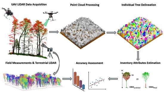
3.2. Global Workflow

The two sub-objectives of this study were achieved using a workflow that includes the following five steps (Figure 5): (1) co-registration of ULS-R and ULS-V data with ALS, TLS, and field inventory data (Section 3.3); (2) detection and delineation of individual trees (Section 3.4); (3) estimation of tree attributes, viz., tree height, CD, and DBH (the latter from either: (a) using an allometric predictive model that input height and CD as predictors; or (b) using a cylinder-fitting procedure on each tree stem (at 1.3 m above the base of the stem)) (Section 3.5); (4) estimation of stand-level attributes, viz., tree count, BA, and DBH-distribution (Section 3.6); and, additionally, (5) sensitivity analysis was performed at the stand-level to evaluate variation of tree count and BA to ITD parametrization that was used in this study (Section 3.7).

3.3. Data Co-Registration

The ALS point cloud was set as the reference dataset for data co-registration as suggested by the provincial government of New Brunswick and adopted by most land managers of the province. ULS-R and ULS-V point clouds were preprocessed, geo-referenced, and co-registered against the ALS point cloud by the data provider (RME Geomatic and Phoenix Aerial Systems, respectively). A three-step procedure was applied to finely co-register the TLS point cloud with the field-inventory tree map and ALS and ULS datasets. First, a tree map was created from the TLS point clouds at 1.3 m AGL following the procedure that was suggested by [38] (Section 3.5.1). Second, coarse registration between TLS point clouds and the field-inventory tree map was performed by: (i) calculating the 3D roto-translation between the two tree maps using the “Iterative Closest Point (ICP)” tool that is available in CloudCompare [92]; and (ii) applying this 3D roto-translation to the TLS point clouds [93]. Third, a fine co-registration between TLS point clouds and the ULS-V geo-referenced point clouds was performed following the “K-4PCS” method used in [94]. This involved reducing the density of TLS point clouds (here set to one point/cm³ using a voxel grid filter) to detect the main 3D key points that were necessary for the fine co-registration process. The latter was performed using the “fine registration (ICP) tool” that is available in CloudCompare. Figure 6 provides an example of the four co-registered datasets stacked together.

3.4. Individual Tree Detection and Delineation (ITD)

The ITD algorithms that were used in this paper had been selected to be representative of the two main categories that are mainly used in the literature to process ALS and TLS data, i.e., raster-based and point cloud-based algorithms, respectively. One algorithm from each category was selected, among a pool of existing ITD algorithms available from recent studies and benchmarks [30,42,43,44,45,76,95,96] to assess their potential and limitations for transferability to ULS point clouds. The raster-based and point-based algorithms that gave the most accurate ITD results when visually compared to the TLS data were selected. As such, the raster-based ITD algorithm SEGMA [97] was selected to process the leaf-on ULS-R point cloud, while the point cloud-based ITD algorithm SimpleTree [36] was selected to process the leaf-off ULS-V point cloud. SEGMA was also applied to the leaf-off ULS-V point cloud to compare the results that were obtained by the two types of ITD algorithms from the same ULS-V raw point cloud (Figure 5). The leaf-on ALS point cloud was also processed using SEGMA to provide an additional comparison between ALS and ULS ITD results. TLS point clouds were processed semi-automatically, using: (i) the SimpleTree algorithm to detect and delineate individual trees; and (ii) CloudCompare software was used to visually inspect SimpleTree results and eventually manually improve tree delineation.

3.4.1. Raster-Based ITD—SEGMA

Individual trees were detected and delineated from ALS, ULS-R, and ULS-V rasterized CHM (hereafter referred to as ALS-Raster, ULS-R-Raster, and ULS-V-Raster, respectively) using SEGMA [30,97], which is a raster-based ITD algorithm developed in Python [98] and implemented in open-source in the Computree platform [99] (Figure 7). SEGMA ITD algorithm works on the CHM and involve six main steps: (i) creation of a pit-free CHM; the resolution of 25 cm was chosen based on [100,101] recommendations; (ii) adaptive Gaussian smoothing of the CHM and identification of its local maxima (Figure 7A); (iii) adaptive filtering of local maxima using exclusion distance criteria to identify tree tops; (iv) watershed delineation of individual tree crowns from the designed tree tops (Figure 7B); (v) iterative refinement of the delineated tree crowns on the basis of geometric quality criteria that were calculated from the crown shape and 3D features; and (vi) top to bottom delineation of trees in the point cloud from the delineated tree crowns (Figure 7C). CHM smoothing is largely controlled by the standard deviation (sigma) of the CHM adaptive Gaussian filter. Higher sigma values lead to stronger CHM smoothing, resulting in a coarser tree crown delineation (and vice-versa). In this study, the sigma value was set to 0.45 (i.e., filter range = 3.46 m) and adjusted iteratively in Computree by visual comparison of the ITD results with the CHM and TLS reference trees.

3.4.2. Point Cloud-Based ITD—SimpleTree

Individual trees from the ULS-V point cloud (hereafter referred to as ULS-V-Pcloud) were detected and delineated using SimpleTree [36], an open-source plugin that was developed in C++ and implemented in the Computree platform (Figure 8). One of the advantages of using SimpleTree for the point cloud-based ITD lies in the fact that it was initially developed and optimized to handle very high-density TLS point clouds with minimal parametrization. Therefore, it is quite fast when processing high-density ULS point clouds (~6 min for 1 ha (1585 points/m²) on a 32 Giga-byte RAM laptop). The SimpleTree ITD algorithm adopts a bottom-up approach, which implies that the stem base is identified first. It then uses this base as a seed to ascend the tree bole and delineate the entire tree. This is achieved by working directly in the raw point cloud (Figure 8A) following four main steps: (i) identification and extraction of vegetation points from the ground and creation of a digital terrain model from the ground points (DTM) (Figure 8A); (ii) extraction and de-noising of a horizontal slice around the DBH and isolation of individual tree stems using spatial Euclidean clustering (Figure 8B); (iii) bottom-up delineation of individual trees using Dijkstra’s algorithm [102] (range set to 0.20 m; see [36,103,104] for a complete description); and (iv) de-noising of each delineated tree using Euclidean Clustering (Figure 8C).

Individual trees from TLS sample plots were detected and delineated with SimpleTree, using the procedure that is described in this section. Parameters were adapted to the higher point density of TLS point clouds. Individual tree delineations also were visually inspected and eventually refined manually in CloudCompare.

3.5. Tree-Level Structural Attributes Estimation

3.5.1. Tree Height and Crown Diameter (CD)

Tree height was computed in SEGMA as the height of the local maximum for each tree that was identified in the ALS-Raster, ULS-R-Raster and ULS-V-Raster datasets (Section 3.4.1). Tree CD was also computed in SEGMA from the crown projected area ($CD=2\times \sqrt{Crown projected area/\pi }$). SEGMA automatically refines its crown delineation process after computing individual tree attributes. To do so, the algorithm assigns a score to each delineated tree based on simple geometric criteria (e.g., minimum point density, ratios between tree height and CD), with eventual removal of erroneously detected trees to improve the ITD [30,97].

Tree height was computed in the R environment [105] for each tree that was delineated by SimpleTree from the ULS-V-Pcloud (Section 3.4.2). To do so, the vertical distance is computed between the highest point of the tree and the ground surface elevation directly beneath it. Tree CD was computed for each tree in R following the method that was proposed by [106] (Figure 9). This method involves five steps for identifying the crown-based height (CBH) of the tree and then computes CD from the projected area of the classified crown points ($CD=2\times \sqrt{Crown projected area/\pi }$) by:

(i)

vertically dividing the tree point cloud into 10-cm height clusters;

(ii)

fitting convex hull polygons to xy-coordinates of each cluster along the tree bole;

(iii)

calculating maximum Euclidean distance between the centroid of each convex hull and its vertices, and plotting the results along the z-axis (Figure 9A);

(iv)

identifying the CBH of the tree by fitting a segmented (piecewise) regression to the plotted points using the Segmented R package [107] (the CBH is defined as the lowest breakpoint (knot) of the segmented regression, which corresponds to the height where the regression slope starts to increase sharply because of the presence of branches) (Figure 9A “Breakpoint”); and

(v)

classifying the points above the CBH as belonging to the crown (Figure 9B), and using them to compute CD.

Each tree crown with unnatural dimensions (i.e., an erroneously delineated tree) was automatically removed based on simple geometric criteria (e.g., minimum point density, ratios between tree height, and CD) to improve SimpleTree ITD.

Tree height from each tree that was delineated from TLS point clouds (Section 3.4.2) was estimated in R by calculating the vertical distance between the highest point of the tree and the ground surface elevation directly below it. Tree CD from each TLS tree was computed following the five-step procedure [106] that is described in this section. We also added a visual inspection step and an eventual manual adjustment of CBH performed in R for a last verification of the estimated TLS tree height and CD.

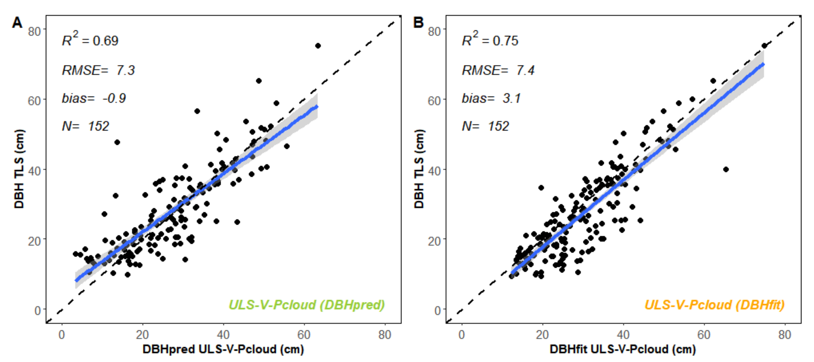
3.5.2. Diameter at Breast Height (DBH)

Three methods were investigated for estimating tree DBH from the delineated trees:

• Predicting DBH using height and CD allometry (Equation (1)) from raster-based ITD trees [28];
• Predicting DBH using height and CD allometry (Equation (1)) from point cloud-based ITD trees [49];
• Estimating DBH using a cylinder-fitting algorithm onto tree stems [39,45,90].

The choice of the approach differed from one dataset to another, and was guided by the level of detail in the point cloud for a given acquisition configuration (Figure 3). Method #2 and method #3 are more restrictive than method #1, as the tree stems need to be recorded in the 3D point cloud for these methods to work. As such, method #2 and method #3 were only assessed on the ULS-V-Pcloud data. ULS-V-Pcloud data was processed with each method (Figure 5): (i) to compare the accuracy of DBH predicted from a point cloud-based ITD and a raster-based ITD (method #1 vs. method #2); and (ii) to compare the accuracy of DBH predicted against DBH fitted with cylinders from the same ULS-V-Pcloud trees (method #2 vs. method #3). The idea behind method #2 is that in some cases, there might be sufficient numbers of points on the stems to allow a bottom-up ITD, but not enough points to perform an accurate cylinder-fitting procedure. The latter deficiency prevents the use of the cylinder-fitting approach, but allows DBH to be predicted through the use of allometric relationships (for example, see [49]).

Predicted DBH (hereafter, referred to as DBH_pred) from ALS-Raster, ULS-R-Raster, ULS-V-Raster, and ULS-V-Pcloud trees was estimated using the model that was proposed by [28], and which was developed for the angiosperm forest type (Nearctic realm). This allometric model was adapted to local conditions using the TLS data. To do so, we performed a gradient descent analysis using Ht, CD, and DBH from the TLS reference trees to refine the model coefficients of the original equation from [28], which resulted in:

$${\mathrm{DBH}}_{pred}=\exp \left[-0.625+0.84ln\left(Ht\times CD\right)\right]+\exp \left({\sigma }^2/2\right),$$

(1)

where $\sigma$² is the mean-square error of the regression, Ht is the tree height (m), and CD is the crown diameter (m).

Fitted DBH (hereafter, referred to as DBH_fit) from ULS-V-Pcloud trees was estimated using the cylinder-fitting algorithm that is available in Computree [34,78,88,108]. The algorithm (Figure 10) proceeds in five main steps: (i) extraction of a stem slice (Figure 10A); (ii) clustering of the stem slice into horizontal clusters (20 cm widths, Figure 10B); (iii) aggregation of clusters into logs, based on their relative vertical and horizontal positions (Figure 10C); (iv) fitting cylinders (50 cm height [109]) onto the log using nonlinear least-squares estimation (Figure 10D); and (v) interpolation of tree DBH from the cylinders around 1.3 m above the ground surface (Figure 10E). Stem location was considered to be the center of the computed DBH_fit. A cylinder-fitting procedure, which was similar to the one used for DBH_fit, was applied to estimate TLS DBH (hereafter, referred to as DBH_TLS), but parameters were adapted to the higher point density of the TLS point cloud.

3.6. Stand-Level Inventory Attribute Estimation

Tree count, BA, and DBH-distribution were respectively estimated, as follows:

$$Tree Count={{\displaystyle \sum }}_{i=1}^n\left(tre{e}_i\right),$$

(2)

$$BA={{\displaystyle \sum }}_{i=1}^n\left(\frac{{({\mathrm{DBH}}_{pred/fi{t}_i})}^2\times \pi }{\mathrm{40,000}}\right),$$

(3)

$$\mathrm{DBH}-distribution=\frac{{{\displaystyle \sum }}_{i=1}^n\left({\mathrm{DBH}}_{pred/fi{t}_i}\right)}{5 \mathrm{cm} class},$$

(4)

where tree_i is the tree that was delineated from the CHM or point cloud (Section 3.4), and DBH_i is the DBH of tree_i that was estimated (Section 3.5.2). These estimates were: (i) DBH_pred, which was predicted from ALS-Raster, ULS-R-Raster ULS-V-Raster, and ULS-V-Pcloud tree_i (Equation (1)); and (ii) DBH_fit, which was estimated from ULS-V-Pcloud tree_i using the cylinder-fitting approach.

3.7. Evaluation Methods

3.7.1. ITD Performance

Tree detection performance was evaluated through two distinct assessment analyses. First, ITD performance was assessed at the stand-level by comparing the number of trees that were detected (hereafter, referred to as ${\mathrm{Ntrees}}_{\det }$) from ALS-Raster, ULS-R-Raster, ULS-V-Raster, and ULS-V-Pcloud (Section 3.4) to the total number of field-measured trees (N = 477). The tree crown polygons that overlapped the boundary of the stand were counted when their local maxima were located inside the stand.

Second, the ITD accuracy was further evaluated as the proportion of ${\mathrm{Ntrees}}_{\det }$ from ALS-Raster, ULS-R-Raster, ULS-V-Raster, and ULS-V-Pcloud that were paired with a TLS tree (hereafter, referred to as ${\mathrm{Ntrees}}_{\mathrm{paired}}$), to the number of TLS trees (N = 258). This second step was only assessed within the TLS sample plots, as the TLS data did not covered the entire study site (see Figure 1). Following forestry inventory standards, a multi-stem tree is considered to be one tree if the beginning of the fork is above 1.3 m AGL. Conversely, it is inventoried as multiple trees if the fork is below 1.3 m AGL. Trees that were identified as multiple trees by the field inventory, but as one tree in the TLS dataset (i.e., 21 trees; 7%), were problematic for validating ITD performance. Therefore, they were excluded from the second analysis.

Our tree matching algorithm that identified ${\mathrm{Ntrees}}_{\mathrm{paired}}$ was implemented in R, and it was derived from the three-step procedure proposed by [43]. We set the TLS tree crown centroid as reference for the matching procedure instead of using the x,y value at the bottom of the stem [43]. This minimized matching errors for tilted or curved stems. Crown centroids of ALS/ULS trees (hereafter, referred to as “test”) were used to test any possible match with TLS tree crown centroids (hereafter, referred to as “reference”). The first step involves “candidate searching”. It sorts test trees by height and the matching procedure processes from the highest to the lowest test tree. Candidate reference trees are determined using the neighborhood criterion ${\mathsf{\Delta }\mathrm{D}}_{2\mathrm{D}}$ and a height criterion ∆H (

Table 2. Height and neighborhood criteria for the candidate search. $H_{Test}$, height of test tree; ∆H, height difference between test (i.e., ALS/ULS tree crown centroid) and reference (i.e., TLS tree crown centroid); ${\mathsf{\Delta }\mathrm{D}}_{2\mathrm{D}}$, 2D distance between test and reference trees.

Criterion	Height Test & Distance Test	Distance Test
1	$H_{test}$ < 10 m & ∆H < 2.5 m	${\mathsf{\Delta }\mathrm{D}}_{2\mathrm{D}}$ < 3 m
2	10 m ≤ $H_{test}$ < 15 m & ∆H < 3 m	${\mathsf{\Delta }\mathrm{D}}_{2\mathrm{D}}$ < 3.5 m
3	$H_{test}$ ≥ 15 m & ∆H < 4 m	${\mathsf{\Delta }\mathrm{D}}_{2\mathrm{D}}$ < 4 m

). The second step involves “candidate voting.” It ranks candidate reference trees based on their ΔH and ${\mathsf{\Delta }\mathrm{D}}_{2\mathrm{D}}$ with the test tree. The reference tree becomes the new best-voted candidate when ΔH is the smallest and ${\mathsf{\Delta }\mathrm{D}}_{2\mathrm{D}}$ is ≤2.5 m from the initial candidates. The third step involves “candidate testing.” This step evaluates the score of all best-voted candidate reference trees against the surrounding test trees. Two trees form a matched pair when the best-voted test tree is the closest tree with the smallest height difference. Search radius distances (Table 2) were determined empirically by testing different settings on a subset of the study site and visually interpreting the quality of the matching results.

3.7.2. Accuracy Assessment on Estimated Attributes

Accuracies of the tree-level estimated attributes (i.e., tree height, CD, and DBH_pred) were evaluated by calculating the root-mean-square error (RMSE), bias, and coefficient of determination (R²):

$$RMSE=\sqrt{\frac{1}{n} {{\displaystyle \sum }}_{i=1}^n{({\hat{y}}_i-y_i)}^2},$$

(5)

$$bias=\frac{1}{n} {{\displaystyle \sum }}_{i=1}^n({\hat{y}}_i-y_i),$$

(6)

$$R^2=1-\frac{{{\displaystyle \sum }}_{i=1}^n{\left({\hat{y}}_i-y_i\right)}^2}{{{\displaystyle \sum }}_{i=1}^n{\left({\overline{y}}_i-y_i\right)}^2},$$

(7)

where $n$ is the number of ${\mathrm{Ntrees}}_{\mathrm{paired}}$ (i.e., number of ${\mathrm{tree}}_{\mathrm{i}}$ detected and paired with their TLS reference tree), ${\hat{y}}_i$ is the estimated attribute for ${\mathrm{tree}}_{\mathrm{i}}$, $y_i$ is the reference TLS attribute that was measured for $tre{e}_i$, and ${\overline{y}}_i$ is the mean of the TLS reference attribute.

The performance of tree DBH_fit from the cylinder-fitting procedure (Section 3.5.2) was achieved by calculating the number of successful fits among the ULS-V-Pcloud ${\mathrm{Ntrees}}_{\mathrm{paired}}$ (N = 183). Furthermore, the accuracy of these successful DBH_fit was assessed against their paired DBH_TLS, and directly compared to DBH_pred that was estimated from the same ULS-V-Pcloud trees.

The accuracies of the stand-level estimated attributes (i.e., tree count, BA, and DBH-distribution) were evaluated against the field measurements, given that TLS data did not cover the entire 1 ha study site. Both stand- and tree-level attributes that were estimated using raster-based ITD are dependent on the level of CHM smoothing (e.g., [110,111]). Therefore, an additional sensitivity analysis was conducted at the stand-level by varying sigma, i.e., the parameter defining the level of CHM smoothing. This was done to assess how the ITD parametrization can affect: (i) tree detection (i.e., in terms of tree count for a given sigma value); (ii) tree delineation accuracy (i.e., in terms of median tree height and median tree CD); and (iii) estimation of stand BA. A summary of the processing techniques that were used for estimating forest inventory attributes is provided in

Table 3. Summary of methods that were used for individual tree detection and delineation (ITD), and for tree DBH estimation from each dataset for a given foliage condition.

Dataset	Canopy Condition		ITD Approach		DBH Approach
	Leaf-On	Leaf-Off	SEGMA	SimpleTree	Predicted	Fitted
ALS-Raster	x		x		x
ULS-R-Raster	x		x		x
ULS-V-Raster		x	x		x
ULS-V-Pcloud				x	x	x
FI & TLS (Ref)		x		x		x

.

4. Results

4.1. ITD Performance

Automatic ITD algorithms over the stand detected 57%–73% of ${\mathrm{Ntrees}}_{\det }$, of which 40% to 71% were ${\mathrm{Ntrees}}_{\mathrm{paired}}$ (

Table 4. Detailed ITD performance that was obtained from each aerial dataset with their main acquisition parameters and the ITD algorithm that was applied. ${\mathrm{Ntrees}}_{\det }$ represents the total number of trees that detected over the stand among the N = 477 trees that were measured in the field inventory (${\mathrm{Ntrees}}_{\mathrm{FI}}$). ${\mathrm{Ntrees}}_{\mathrm{paired}}$ represents the number of ${\mathrm{Ntrees}}_{\det }$ that formed matched pairs with the N = 258 TLS reference trees (${\mathrm{Ntrees}}_{\mathrm{TLS}}$) and are presented by height class.

Dataset	Acquisition Parameters	ITD Approach	$Ntree{s}_{det}$	$Ntree{s}_{paired}$ by Height Class
				[6–12[ m	[12–18[ m	≥18 m	Total
ALS-Raster	Leaf-on (27 pts/m2)	SEGMA	275 (58%)	2 (5%)	18 (15%)	88 (91%)	108 (42%)
ULS-R-Raster	Leaf-on (353 pts/m2)	SEGMA	273 (57%)	1 (2%)	15 (13%)	87 (90%)	103 (40%)
ULS-V-Raster	Leaf-off (1585 pts/m2)	SEGMA	346 (73%)	4 (9%)	28 (24%)	96 (99%)	128 (50%)
ULS-V-PCloud		SimpleTree	340 (71%)	22 (51%)	70 (59%)	91 (94%)	183 (71%)
FI & TLS (ref)	Leaf-off (60 k pts/m2)	SimpleTree & Manual ITD	477 ${\mathrm{Ntrees}}_{\mathrm{FI}}$	43 ${\mathrm{Ntrees}}_{\mathrm{TLS}}$	118 ${\mathrm{Ntrees}}_{\mathrm{TLS}}$	97 ${\mathrm{Ntrees}}_{\mathrm{TLS}}$	258 ${\mathrm{Ntrees}}_{\mathrm{TLS}}$

). The best ITD performance was obtained from the ULS-V-Pcloud dataset that was acquired in leaf-off conditions using the SimpleTree bottom-up ITD (Figure 11D), with a total of 71% ${\mathrm{Ntrees}}_{\det }$ and 71% ${\mathrm{Ntrees}}_{\mathrm{paired}}$ (Table 4). The best raster-based ITD performance was achieved in leaf-off conditions on ULS-V-Raster, with a total of 73% ${\mathrm{Ntrees}}_{\det }$ and 50% ${\mathrm{Ntrees}}_{\mathrm{paired}}$.

Point density differences between ULS-R (353 points/m², Figure 11A) and ALS point cloud (27 points/m², Figure 11B), which were both collected under leaf-on conditions, did not change performance of the raster-based ITD for either ${\mathrm{Ntrees}}_{\det }$ (58% and 57%, respectively) or ${\mathrm{Ntrees}}_{\mathrm{paired}}$ (42% and 40%, respectively). A significant difference between ${\mathrm{Ntrees}}_{\det }$ was observed for leaf-on ULS-R-Raster (57%, Figure 11B; Table 4) versus leaf-off ULS-V-Raster (73%, Figure 11C; Table 4). However, a smaller difference was noted for ${\mathrm{Ntrees}}_{\mathrm{paired}}$ with 40% for leaf-on ULS-R-Raster and 50% for leaf-off ULS-V-Raster. Again, the difference in point density between these two datasets (353 points/m² and 1585 points/m², respectively) does not seems to have a major impact on the raster-based ITD results (Table 4).

ITD algorithms were further assessed for their ability to detect trees from multiple canopy layers using the TLS trees as reference (Figure 12; Table 4). Both point cloud-based and raster-based ITD were efficient for detecting trees in the upper canopy (over 90% of ${\mathrm{Ntrees}}_{\mathrm{paired}}$ ≥ 18 m height, for all datasets). However, the ability of raster-based ITD to detect trees in the intermediate (12–18 m height class) and lower canopy layers (6–12 m height class) was gradually lower, with detection rates varying from 13% to 24% and from 2% to 9%, respectively. The graphical comparison of ULS-V-Pcloud and ULS-V-Raster distributions of ${\mathrm{Ntrees}}_{\mathrm{paired}}$ (Figure 12) shows that the point cloud-based ITD (${\mathrm{Ntrees}}_{\mathrm{paired}}$ = 71%) outperformed the raster-based ITD (${\mathrm{Ntrees}}_{\mathrm{paired}}$ = 50%). Substantial improvements also occurred in both intermediate canopy layers (${\mathrm{Ntrees}}_{\mathrm{paired}}$ = 51% with ULS-V-Pcloud vs. ${\mathrm{Ntrees}}_{\mathrm{paired}}$ = 24% with ULS-V-Raster) and lower canopy layers (${\mathrm{Ntrees}}_{\mathrm{paired}}$ = 51% ULS-V-Pcloud vs. ${\mathrm{Ntrees}}_{\mathrm{paired}}$ = 9% with ULS-V-Raster). These results demonstrate the potential of the ULS-V-Pcloud to detect trees belonging to different canopy layers.

4.2. Tree-Level Structural Attribute Accuracy

Tree height was estimated with high accuracy from all aerial datasets, with R² values between 0.8 and 0.9 and bias less than 1 m (Figure 13A). Poor CD estimates were found for ALS-Raster, ULS-R-Raster, and ULS-V-Raster datasets, with R² values of 0.22, 0.24, and 0.29, respectively (Figure 13(B1–B3)). No major difference in CD estimation accuracy was found between ALS-Raster that was constructed from the 27 points/m² ALS point cloud (R² = 0.22, Figure 13(B1)) and ULS-R-Raster that was constructed from the 353 points/m² ULS-R point cloud (R² = 0.24, Figure 13(B2)); both were acquired under leaf-on conditions. A slight improvement in CD estimation accuracy was observed for leaf-off ULS-V-Raster (R² = 0.29, Figure 13(B3)), compared to the leaf-on ULS-R-Raster (R² = 0.24, Figure 13(B2)). Yet this improvement comes at the cost of decreasing delineation accuracy of large crowns (Figure 13(B3)), compared to leaf-on data (Figure 13(B2)). The most accurate estimates of CD were found when using the bottom-up, point cloud-based ITD on leaf-off ULS-V-Pcloud (Figure 13(B4)). The latter improved CD estimates from R² = 0.29 (Figure 13(B3)) from ULS-V-Raster to R² = 0.61 from ULS-V-Pcloud (Figure 13(B4)).

DBH_pred estimated from method #1 (Section 3.5.2) by using tree height and CD from ALS-Raster, ULS-R-Raster, and ULS-V-Raster (Equation (1)), performed poorly against the reference DBH_TLS, with similar RMSE of 12.2 cm, 11.8 cm, and 11.5 cm, respectively (Figure 13(C1–C3)). DBH_pred estimated from method #2 (Section 3.5.2) using tree height and CD from the bottom-up ULS-V-Pcloud yielded the best estimates against DBH_TLS, with a RMSE of 7.7 cm (Figure 13(C4)). The graphical assessment of DBH_pred from ULS-V-Raster (R² = 0.36, Figure 13(C3)) and ULS-V-Pcloud (R² = 0.67, Figure 13(C4)) illustrates the benefits of using a bottom-up ITD compared to a raster-based ITD for improving DBH_pred accuracy.

Method #3 (Section 3.5.2), which fits cylinders onto tree stems automatically, identified 152 DBH_fit among the 183 ULS-V-Pcloud ${\mathrm{Ntrees}}_{\mathrm{paired}}$. The accuracy of these DBH_fit values was assessed against their paired DBH_TLS (Figure 14B) and compared to DBH_pred from the same 152 ULS-V-Pcloud trees (Figure 14A). Similar accuracy was obtained between DBH_pred (RMSE = 7.3 cm) and DBH_fit (RMSE = 7.4 cm), highlighting the great potential of both approaches for estimating tree DBH from bottom-up ITD trees. Yet, DBH_fit led to greater bias (3.1 cm), resulting in overestimation of small-sized trees (DBH < 30 cm) and underestimation of large-sized trees (DBH > 50 cm). In contrast, DBH_pred led to a lower bias −0.9 cm), resulting mainly in the underestimation of large-sized trees (DBH > 50 cm) (Figure 14A).

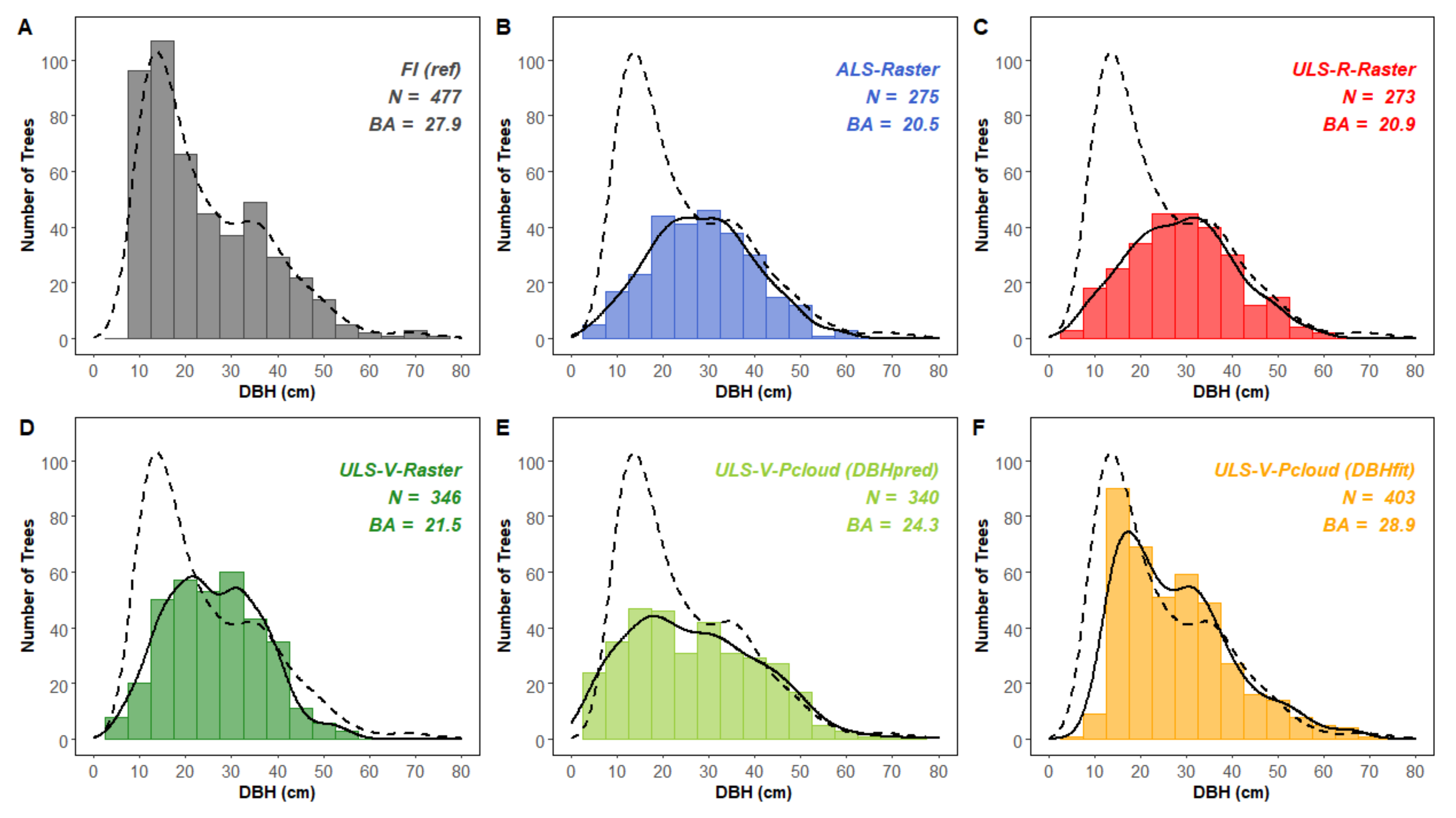
4.3. Stand-Level Inventory Attribute Accuracy

The tree count estimated from all datasets and methods was significantly lower relative to the reference value, especially when using raster-based ITD. The closest estimate of tree count was obtained using method #3 on the ULS-V-Pcloud, i.e., using the point cloud-based ITD and the cylinder-fitting approach (84% of trees detected, i.e., 403 out of 477 trees; Figure 15F).

BA estimates were systematically underestimated using the predictive modeling (method #1), by −26.6% for ALS-Raster (Figure 15B), −25.1% for ULS-R-Raster (Figure 15C), −22.9% for ULS-V-Raster (Figure 15D) and −12.9% for ULS-V-Pcloud (DBH_pred) (Figure 15E). Conversely, BA was slightly overestimated (+3.5%) using the cylinder-fitting (method #3) on ULS-V-Pcloud (DBH_fit) (Figure 15F), which turned out to be the closest estimate of stand BA.

DBH-distribution of trees in 5-cm class increments (Figure 15) showed good estimates of large-sized trees (DBH > 35 cm), for all datasets and approaches. Yet, the ALS-Raster, ULS-R-Raster, and ULS-V-Raster DBH-distributions failed to represent the typical field-measured inverse J-shaped DBH-distribution. This is mainly due to trees that were missing in the lower and intermediate size-classes (10 cm < DBH ≤ 30 cm). Instead, the estimated DBH-distribution approached a unimodal shape that was similar to a Gaussian curve. The ability to detect small-sized DBH trees improved gradually with the successive use of the following datasets: ALS-Raster, ULS-R-Raster, ULS-V-Raster, and ULS-V-PCloud (DBH_pred and DBH_fit). Although slightly right-biased with respect to the field reference, the ULS-V-Pcloud DBH_fit–distribution yielded the most accurate representation of the DBH-distribution shape (Figure 15F). This concurs with the tree-level DBH accuracy assessment presented in Figure 13C.

4.4. Sensitivity Analysis

A sensitivity analysis was applied to assess how the sigma parameter of the SEGMA Gaussian filter affect estimates from ALS-Raster, ULS-R-Raster, and ULS-V-Raster of tree count, median tree height, median tree crown diameter, and BA over the stand (Figure 16). Graphical representation of stand attributes revealed that on the one hand, a higher sigma value resulted in detection of fewer trees (Figure 16A) and the delineation of larger crowns (Figure 16C). On the other hand, tree height (Figure 16B) and BA estimates (Figure 16D) were much less affected by the sigma value than was tree count or crown diameter. Sigma slowly affected tree height estimation.

5. Discussion

5.1. Transferability of ITD Algorithms to ULS Data

Our first specific objective focused on assessing transferability of point cloud-based and raster-based ITD algorithms (SimpleTree and SEGMA, respectively) to an uneven-aged hardwood stand that was surveyed during leaf-on and leaf-off conditions. Our results demonstrated transferability of both ITD to ULS data under certain conditions.

In leaf-off conditions, SimpleTree achieved the best ITD performance on ULS-V data, detecting 71% of the trees in the stand, with 71% of the trees correctly paired with TLS reference trees. Applying SEGMA to the same dataset was less efficient, with 73% of trees detected over the stand, but for only 50% of the trees that were correctly paired with TLS reference trees. This situation was caused by false positive tree detection from the CHM. Three main advantages were identified using SimpleTree ITD on leaf-off ULS-V data, compared to SEGMA. First, it provides substantial improvement for the detection of trees in the low (9% with SEGMA; 51% with SimpleTree) and intermediate canopy layers (24% with SEGMA; 59% with SimpleTree), while providing comparable detection of trees in the uppermost canopy layer (99% with SEGMA; 94% with SimpleTree) (Figure 12, Table 4). Second, SimpleTree minimized hardwood tree crown over- and under-delineation problems, providing better estimates of CD (Figure 13). Thirdly, bottom-up ITD like SimpleTree provide information on both tree morphology (Figure 10) and crown dimensions (Figure 9), which in turn can be used to model additional attributes currently not exploited by conventional raster-based ITD.

Three main limitations were encountered transferring SimpleTree onto ULS-V data. First, trees with relatively low point densities along the boles may be omitted. Second, isolating ULS tree stems from the surrounding vegetation is more complex than for TLS point clouds. Indeed, as point distributions along the stem are less dense and more scattered than for TLS point clouds [36], the edges of tree stems are less well defined and more easily confused with low vegetation during the de-noising procedure. Adapting the de-noising procedure for the ULS point cloud implies tradeoffs where point filtering must be strong enough to suppress understory noise, but not so strong as to avoid filtering out smaller-sized stems. Third, SimpleTree is more computationally intensive than conventional raster-based ITD; up to 6 min may be required to process a 1 ha ULS-V point cloud (1585 points/m²), instead of a few seconds for applying a raster-based method to the same area.

Awareness of limitations that are related to processing ULS data can facilitate applying specific procedures to maximize results. For instance, one way to overcome the two first limitations is to fly the ULS in in parallel lines crossing at 90° to obtain multiple views of all areas. This pattern reduces signal occlusion and facilitates de-noising, thereby improving tree detection in the lower canopy layers. Increasing the point density during data acquisition may also help improve bottom-up ITD results. For most methods that have been developed for point cloud processing, the computation time follows an exponential growth curve with increased data size due to computational complexity [112]. This suggests an important trade-off: ULS point density must be high enough to locate individual stems and possibly use geometric fitting, but it must be kept to a reasonable level to avoid lengthy processing times. We showed that a point density of about 1500 points/m² already yielded good bottom-up ITD performance. Constraints on processing may require applying bottom-up ITD only on small areas or partitioning large forested areas into separate tiles. Last, another possible solution for improving bottom-up ITD performance would combine automated stem detection with canopy segmentation (e.g., [113,114,115]).

Despite the abovementioned limitations, an increasing number of studies have demonstrated that bottom-up ITD on high-density aerial LiDAR data are more suitable for processing complex hardwood forests than conventional raster-based ITD (see [22,49,116]). Improving ITD by integrating a stem detection step from high-density aerial LiDAR data is still an active research topic (e.g., [22,49,114,115,116,117]). From an application point of view, collecting ULS data in leaf-off hardwood stands supports a wide array of tree-level analyses, such as selective logging [118], allometric model development [119], tree stem modeling [62], tree species identification [120], health and vigor evaluation [121], or tree competition [122]. One aspect that seems particularly important to explore further is the use of deep learning analysis for species identification from bottom-up ITD trees from high-density ULS [123]. Integrating ULS data with TLS data could also be further studied for estimating the biomass of individual trees.

In leaf-on conditions, substantial LiDAR signal occlusion from the upper canopy on dense canopy foliage of hardwood trees is an unavoidable constraint of aerial systems [124]. Although the ULS-R system collected up to 7 returns per pulse with an average point density of 353 points/m², most tree stems were missed and trees from the intermediate and lower canopy layers were hardly identifiable (Figure 3B and Figure 11B). Under these circumstances, the raster-based ITD SEGMA was more efficient than point cloud-based ITD. This was also observed by [59]. SEGMA results obtained from leaf-on data are comparable to ALS-based ITD performance over heterogeneous forest, where typical tree detection ranged from 40% to 80% (see [22,30,43,44] reviews). Interestingly, similar performances were achieved by SEGMA on ALS (27 points/m²) and ULS-R (353 points/m²) point clouds, which were both collected under similar foliage conditions (Figure 12, Table 4). In our analysis, an increase in point density with the ULS-R did not improve raster-based ITD performance. A similar conclusion was reported in [117].

The main limitation of SEGMA that was applied to the uneven-aged hardwood stand is its inability to detect understory trees, which is mainly caused by the loss of 3D information when oversimplifying the point cloud into a CHM [20,32]. This led to poor results in lower (around 5%) and intermediate (15%) canopy layers, for both ALS and ULS-R data (Figure 12, Table 4). Similar detection rates were reported in the ITD benchmark of [43] in heterogeneous forests. These results illustrate an important limitation of the raster-based ITD in supporting uneven-aged hardwood forest interventions and assist-harvesting activities, especially for applications requiring information on successional forest stages.

A potential way to overcome raster-based ITD inability to detect understory trees from leaf-on hardwood forests is to develop hybrid approaches that combine raster and point cloud-based ITD (e.g., [125]). Algorithms such as 3D adaptive mean shift clustering ITD also show great promise for detecting trees in uneven-aged forested areas (e.g., [20,31,126]). However, their transferability to various forest types is still experimental. Future studies should therefore investigate their potential for transferability to ULS data from a variety of forest stands. Integrating methods that can delineate or merge trees based on the analysis of similarities between segments (e.g., [113,117]) and their assignment to a specific canopy layer also present some potential for processing high-density point clouds (e.g., [20,127]). Last, including some evaluation criteria that are based on dendrometric criteria and machine learning (e.g., [123,128]) should also be further explored to really benefit from gleaning the full information that is available in high density ULS data.

5.2. Forest Inventory Attributes of an Uneven-Aged Hardwood Stand Using ULS Data

The second specific objective of this study was to compare automated methods for the retrieval of forest inventory attributes at the tree-level (i.e., height, crown diameter (CD), DBH) and at the stand-level (i.e., tree count, BA, DBH-distribution). We observed that LiDAR point cloud properties strongly influenced the methodological choices for ITD and attribute estimation. Leaf-on and leaf-off conditions lead to specific and distinct methods for estimating inventory attributes. Overall, three methods stand out based on DBH estimation from point cloud properties (Figure 5). These include:

• Predicting DBH using height and CD allometry (Equation (1)) from raster-based ITD trees;
• Predicting DBH using height and CD allometry (Equation (1)) from point cloud-based ITD trees;
• Estimating DBH using cylinder-fitting algorithm.

Method #1 is the most commonly-used approach for processing ALS data. It aims to detect and delineate individual trees based on the CHM, and it uses allometric models to predict DBH. This method does not require very high-density point clouds to work and there is no need to identify the stems in the point cloud. DBH prediction depends on the accuracy of tree height and CD predictors (Equation (1)) that are derived from the CHM. The authors of [129] achieved relatively good DBH prediction with this method in Norwegian boreal coniferous forests and temperate forests in the Italian Alps (RMSE of 5.17–5.39 cm and 9.9 cm, respectively). Our results were less accurate, for both the ULS-R point cloud and ALS point cloud (RMSE of about 12 cm; Figure 13(C1–C3)). Dominance of hardwood trees in our study explains these differences. Crown apices of hardwood trees are more difficult to detect and tree boundaries are less evident than for coniferous trees (typically exhibiting “crown shyness”), leading to poorer ITD performance when the stand is dominated by hardwoods [95,130]. The low accuracy of tree CD estimates that were obtained for all airborne sensors (Figure 13B) using the raster-based ITD algorithm also confirms this tendency. Since tree heights were accurately estimated (Figure 13A), we assume that the poor prediction of tree DBH_pred was mostly caused by the estimation of CD, combined with uncertainties of the allometric model. Our findings accord with those of [28,130], who identified that the greatest constraint of using height and CD predictive models is finding reliable ITD algorithms from aerial point clouds.

At the stand-level, method #1 resulted in underestimation of BA from about 25% for both ALS and ULS-R datasets (Figure 15B,C). BA estimation is based on all individual tree DBHs in the stand. Its underestimation can therefore be explained by an underestimation of tree numbers by the ITD, underestimation of tree DBH by the allometric model, or both. We found that BA underestimation was slightly attenuated when using leaf-off ULS-V data (Figure 15D). Under leaf-off conditions, LiDAR penetrates deeply into the canopy cover, thereby improving the detection of understory trees [130]. However, the increase of LiDAR pulse penetration also results in more gaps within larger crowns, resulting in detection of multiple crowns for a single large tree [130]. As a result, overestimation of the number of intermediate-sized trees and underestimation of large-sized trees compared to the field reference is observed and explains the differences between leaf-on and leaf-off predicted DBH-distribution. Considering our results, method #1 seems mostly limited to estimating BA of dominant hardwood trees (Figure 15). Interestingly, our results also show that although BA was underestimated, its value was quite robust with respect to the sigma parameter controlling the strength of the Gaussian filter that was applied to the CHM (Figure 16D). Graphical assessment of Figure 16 showed us that this stable behavior of BA is mainly due to a compensation effect between the number of trees detected and their CD for a given sigma value. A low sigma value leads to the detection of many trees of smaller CD dimensions, while a high sigma value leads to the detection of fewer trees with larger CDs, resulting in comparable estimates of BA. In addition to improving tree DBH_pred accuracy [28], this shows that integrating CD into the allometric equation may also improve stand BA robustness relative to variation in sigma values when raster-based ITD are used. One way to improve estimates of BA is to integrate a theoretical DBH model (e.g., [131]) or an algorithm to match histogram distributions (e.g., [132]). Another alternative is the use of other types of ITD algorithms that are better adapted to the detection of understory trees (e.g., [133]), but their transferability to various forest types is still experimental.

Method #2 is more restrictive than method #1 because it requires stems to be identified in the point cloud for the bottom-up ITD to work. This method must therefore be favored when dealing with point clouds in which stems were completely or partially recorded (e.g., [22,49]). Method #2 minimizes crown delineation problems when compared with method #1. Compared to the raster-based ITD, the bottom-up ITD improved CD estimates from R² = 0.29 to R² = 0.61 on the same ULS-V raw data, when compared to TLS CD. This resulted in improving DBH prediction from RMSE of 11.5 cm to RMSE of 7.7 cm, compared to DBH_TLS.

At the stand-level, method #2 improved BA estimation, but still underestimated it by 12.9% (Figure 15E). Improved prediction of intermediate and large-size trees DBH-distribution (Figure 15D) minimized BA underestimation when compared to method #1. Yet, the remaining BA underestimation was caused by the omission of understory trees while applying the point cloud-based ITD. A drawback of method #2 is the difficulty in dealing with multi-stemmed hardwood trees. We found that during seed identification at the base of tree stems, some multi-stemmed trees were identified as one unique tree by the bottom-up ITD, but as multiple trees by the field inventory. This resulted in some discrepancies in the extreme of the predicted DBH-distribution. We do recommend that efforts should be put into algorithm refinement to deal with multi-stemmed trees. One possible solution is to integrate additional steps that cluster crowns from multi-stemmed trees based on stem section analysis to refine their DBH_pred (e.g., [114,115]).

Method #3 can only be applied under the most restrictive point cloud properties requiring a high-density point cloud; the base of tree stems must be clearly identifiable to apply the cylinder-fitting algorithm [72]. Therefore, this method can mostly be applied when acquiring high-density ULS data under leaf-off conditions. Method #3 does not require allometry; therefore, it avoids predictive model error propagation. Cylinder fitting performed well, with 83% of tree DBH_fit automatically fitted with accuracy comparable with DBH_pred that was obtained using method #2. However, compared to method #2, the cylinder-fitting approach produced greater bias for large-size trees and coarser estimates for small-size trees (DBH ≥ 30 cm and <30 cm, respectively). Our results align closely with recent papers [57,79], suggesting that even if ULS data showed great potential for DBH estimation with the cylinder-fitting approach, uncertainties are still too high at the tree-level to reach field inventory standards. Most of the uncertainties that we found are related to the greater beam divergence of the ULS sensor (e.g., footprint size of the Velodyne HD32-e sensor ranges up to 2.5 cm in this study), compared to TLS. This generally translates into sparser points being recorded around the stem edges, which in turn leads to some DBH overestimation during the cylinder-fitting process (as reported in [79]). Improving our results may require introducing a correction factor or developing integrating algorithms that can account for occlusion, and which are capable of dealing with complex stem structures in the cylinder-fitting process, should be further investigated to improve the results (e.g., [37,134]). Another limitation relates to signal occlusion problems that may occur at the stem-level. One way to overcome this limitation is to use long cylinders during the fitting process, as was used in this study. Our study has led us to suggest three additional recommendations that would maximize the DBH-fitting algorithm efficiency on ULS point clouds: (i) use a laser scanner with a narrower beam divergence and a higher ranging accuracy when possible; (ii) use a cylinder-fitting algorithm that takes into account tree structures such as tapering, branching or curvature to avoid DBH overestimation; and (iii) add a post-processing step that includes allometric rules for identifying and correcting gross errors that could occur on complex forked stems or stems with non-circular shapes. It is also important to note that the cylinder-fitting algorithm process may not be as successful in coniferous stands. Indeed, although data collection in leaf-off conditions allowed us to mitigate the effects of occlusion on deciduous trees, the problem of occlusion remains important when considering coniferous stands [57]. At this stage, the use of semi-automatic approaches, which include some manual supervision, are recommended to avoid gross errors that may be incurred during automated DBH_fit procedures.

At the stand-level, the cylinder-fitting method yielded the most accurate estimates of BA, overestimating it by only 3.5% compared to field measurements (Figure 15F). Two major improvements were found when compared to method #2: (i) error accumulation from allometry is avoided; and (ii) most of multi-stemmed trees are dealt with, as the fitting algorithm was able to discern individual tree stems and fit multiple cylinders when required. Another clear advantage of method #3 compared to predictive modeling is its ability to extract accurate stem positions. In general, cylinder fitting from leaf-off ULS data appears more suitable for supporting operations that require accurate tree maps and a good representation of the DBH-distribution of the stand.

Overall, our study demonstrated the importance of choosing a priori the point cloud properties and consequently the characteristics of the UAV flight before ULS acquisition because these will define which general method can be used. Important improvements in ITD and attribute estimation accuracy were observed when the point cloud is sufficiently detailed to apply the point cloud-based (bottom-up) methods when compared with the raster-based (top-down) methods. Taking advantage of ULS data can be tied to the ability to apply the bottom-up methods. Further studies should evaluate the applicability of the methods investigated when applied to younger or older hardwood forest before more general conclusions can be drawn.

6. Conclusions

Tree-based forest management has gained interest with the development of high-resolution remote sensing data. However, some important challenges remain for the extraction of inventory attributes in the presence of irregular hardwood canopy. The emergence of ULS systems brings new types of 3D point clouds, which need to be studied to better understand how they can support forest inventories. This study was designed to explore different types of ITD algorithms and compare methodological approaches for the extraction of tree and stand-level inventory attributes. We demonstrated, under certain conditions, the transferability of ITD algorithms that were initially developed for ALS and TLS data to ULS data. Under leaf-on conditions, we showed that the physical limits of occlusion by the dense cover of hardwood trees is an important constraint on the application of ITD and attribute estimation methods to ULS data. Accurate tree delineation of hardwood tree crowns is especially challenging. In these conditions, allometric models (DBH = f(Ht × CD)) from raster-based ITD trees led to relatively large crown delineation uncertainties and poor DBH predictions. In this paper, we showed that one way to overcome ITD uncertainties in hardwood forests was applying bottom-up methods to high-density ULS data that were acquired in leaf-off conditions. Bottom-up ITD algorithms such as SimpleTree can be applied when individual tree crowns and stems are clearly identifiable in the point cloud. The results from the bottom-up method outperformed the raster-based ITD SEGMA for tree detection, tree delineation, and prediction of tree DBH. Furthermore, high-density ULS data in leaf-off conditions are suitable for performing cylinder-fitting methods for the retrieval of DBH. Unfortunately, the accuracy of cylinder fitted DBH is still beyond acceptable for field inventory standards. Imminent improvement in the technical specification of portable LiDAR sensors would provide narrower beams and higher ranging accuracy. These improvements will translate to improvements in ITD and attribute estimation accuracy. Given that ULS sensors are becoming more affordable, additional studies evaluating available methods are required to test them under a wide range of forest conditions before more general conclusions can be drawn. Overall the use of a bottom-up ITD on leaf-off ULS point clouds demonstrate a strong potential for overcoming ITD limitations that are currently encountered when using raster-based methods in hardwood stands. Further developments in tree mapping and estimates of crown or stem structural attributes can take place using ULS data that are taken during leaf-off conditions, because canopy occlusion under leaf-on conditions on any above-crown LiDAR data is strongly limiting any method’s improvement. From a management perspective, leaf-off ULS acquisition may open up new opportunities for developing local allometric models, feed up deep learning analysis for species identification, and assist precision harvesting operations.

References

1. Church, R.L.; Murray, A.T.; Barber, K.H. Forest Planning at the Tactical Level. Ann. Oper. Res. 2000, 95, 3–18. [Google Scholar] [CrossRef]
2. Andersson, D. Approaches to Integrated Strategic/Tactical Forest Planning. 2005, pp. 1–29. Available online: https://pub.epsilon.slu.se/928/ (accessed on 12 February 2019).
3. Luoma, V.; Saarinen, N.; Wulder, M.A.; White, J.C.; Vastaranta, M.; Holopainen, M.; Hyyppä, J. Assessing Precision in Conventional Field Measurements of Individual Tree Attributes. Forests 2017, 8, 38. [Google Scholar] [CrossRef] [Green Version]
4. Brang, P.; Spathelf, P.; Larsen, J.B.; Bauhus, J.; Bončína, A.; Chauvin, C.; Drössler, L.; García-Güemes, C.; Heiri, C.; Kerr, G.; et al. Suitability of Close-to-Nature Silviculture for Adapting Temperate European Forests to Climate Change. Forestry 2014, 87, 492–503. [Google Scholar] [CrossRef] [Green Version]
5. Diaci, J.; Kerr, G.; O’Hara, K. Twenty-First Century Forestry: Integrating Ecologically Based, Uneven-Aged Silviculture with Increased Demands on Forests. Forestry 2011, 84, 463–465. [Google Scholar] [CrossRef] [Green Version]
6. Banaś, J.; Ziȩba, S.; Bujoczek, L. An Example of Uneven-Aged Forest Management for Sustainable Timber Harvesting. Sustainability 2018, 10, 3305. [Google Scholar] [CrossRef] [Green Version]
7. Nolet, P.; Kneeshaw, D.; Messier, C.; Béland, M. Comparing the Effects of Even- and Uneven-Aged Silviculture on Ecological Diversity and Processes: A Review. Ecol. Evol. 2018, 8, 1217–1226. [Google Scholar] [CrossRef]
8. Leak, W.B.; Yamasaki, M.; Holleran, R. Silvicultural Guide for Northern Hardwoods in the Northeast. General Technical Report NRS-132; United States Department of Agriculture: Delaware, OH, USA, 2014; p. 46. Available online: https://www.nrs.fs.fed.us/pubs/45874 (accessed on 20 June 2020).
9. Næsset, E. Practical Large-Scale Forest Stand Inventory Using a Small-Footprint Airborne Scanning Laser. Scand. J. For. Res. 2004, 19, 164–179. [Google Scholar] [CrossRef]
10. Bouvier, M.; Durrieu, S.; Fournier, R.A.; Renaud, J.P. Generalizing Predictive Models of Forest Inventory Attributes Using an Area-Based Approach with Airborne LiDAR Data. Remote Sens. Environ. 2015, 156, 322–334. [Google Scholar] [CrossRef]
11. White, J.C.; Tompalski, P.; Vastaranta, M.; Wulder, M.A.; Saarinen, N.; Stepper, C.; Coops, N.C. A Model Development and Application Guide for Generating an Enhanced Forest Inventory Using Airborne Laser Scanning Data and an Area-Based Approach. 2017. Available online: https://cfs.nrcan.gc.ca/publications?id=38945 (accessed on 10 January 2019).
12. Woods, M.; Pitt, D.; Penner, M.; Lim, K.; Nesbitt, D.; Etheridge, D.; Treitz, P. Operational Implementation of a LiDAR Inventory in Boreal Ontario. For. Chron. 2011, 87, 512–528. [Google Scholar] [CrossRef]
13. Treitz, P.; Lim, K.; Woods, M.; Pitt, D.; Nesbitt, D.; Etheridge, D. LiDAR Sampling Density for Forest Resource Inventories in Ontario, Canada. Remote Sens. 2012, 4, 830–848. [Google Scholar] [CrossRef] [Green Version]
14. Brandtberg, T.; Warner, T.A.; Landenberger, R.E.; McGraw, J.B. Detection and Analysis of Individual Leaf-off Tree Crowns in Small Footprint, High Sampling Density Lidar Data from the Eastern Deciduous Forest in North America. Remote Sens. Environ. 2003, 85, 290–303. [Google Scholar] [CrossRef]
15. Hyyppä, J.; Kelle, O.; Lehikoinen, M.; Inkinen, M. A Segmentation-Based Method to Retrieve Stem Volume Estimates from 3-D Tree Height Models Produced by Laser Scanners. IEEE Trans. Geosci. Remote Sens. 2001, 39, 969–975. [Google Scholar] [CrossRef]
16. Popescu, S.C.; Wynne, R.H.; Nelson, R.F. Measuring Individual Tree Crown Diameter with Lidar and Assessing Its Influence on Estimating Forest Volume and Biomass. Can. J. Remote Sens. 2003, 29, 564–577. [Google Scholar] [CrossRef]
17. Popescu, S.C. Estimating Biomass of Individual Pine Trees Using Airborne Lidar. Biomass Bioenergy 2007, 31, 646–655. [Google Scholar] [CrossRef]
18. Yao, W.; Krzystek, P.; Heurich, M. Tree Species Classification and Estimation of Stem Volume and DBH Based on Single Tree Extraction by Exploiting Airborne Full-Waveform LiDAR Data. Remote Sens. Environ. 2012, 123, 368–380. [Google Scholar] [CrossRef]
19. Gleason, C.J.; Im, J. Forest Biomass Estimation from Airborne LiDAR Data Using Machine Learning Approaches. Remote Sens. Environ. 2012, 125, 80–91. [Google Scholar] [CrossRef]
20. Ferraz, A.; Bretar, F.; Jacquemoud, S.; Gonçalves, G.; Pereira, L.; Tomé, M.; Soares, P. 3-D Mapping of a Multi-Layered Mediterranean Forest Using ALS Data. Remote Sens. Environ. 2012, 121, 210–223. [Google Scholar] [CrossRef]
21. Coomes, D.A.; Dalponte, M.; Jucker, T.; Asner, G.P.; Banin, L.F.; Burslem, D.F.R.P.; Lewis, S.L.; Nilus, R.; Phillips, O.L.; Phua, M.H.; et al. Area-Based vs Tree-Centric Approaches to Mapping Forest Carbon in Southeast Asian Forests from Airborne Laser Scanning Data. Remote Sens. Environ. 2017, 194, 77–88. [Google Scholar] [CrossRef] [Green Version]
22. Lu, X.; Guo, Q.; Li, W.; Flanagan, J. A Bottom-up Approach to Segment Individual Deciduous Trees Using Leaf-off Lidar Point Cloud Data. ISPRS J. Photogramm. Remote Sens. 2014, 94, 1–12. [Google Scholar] [CrossRef]
23. Zhen, Z.; Quackenbush, L.J.; Zhang, L. Trends in Automatic Individual Tree Crown Detection and Delineation-Evolution of LiDAR Data. Remote Sens. 2016, 8, 333. [Google Scholar] [CrossRef] [Green Version]
24. Lindberg, E.; Holmgren, J. Individual Tree Crown Methods for 3D Data from Remote Sensing. Curr. For. Rep. 2017, 3, 19–31. [Google Scholar] [CrossRef] [Green Version]
25. Maltamo, M.; Næsset, E.; Vauhkonen, J. Forestry Applications of Airborne Laser Scanning: Concepts and Case Studies. Manag. Ecosyst. 2014, 27, 2014. [Google Scholar]
26. Chen, Q.; Baldocchi, D.; Gong, P.; Kelly, M. Isolating Individual Trees in a Savanna Woodland Using Small Footprint Lidar Data. Photogramm. Eng. Remote Sens. 2006, 72, 923–932. [Google Scholar] [CrossRef] [Green Version]
27. Koch, B.; Heyder, U.; Weinacker, H. Detection of Individual Tree Crowns in Airborne LIDAR Data. Photogramm. Eng. Remote Sens. 2006, 72, 357–363. [Google Scholar] [CrossRef] [Green Version]
28. Jucker, T.; Caspersen, J.; Chave, J.; Antin, C.; Barbier, N.; Bongers, F.; Dalponte, M.; van Ewijk, K.Y.; Forrester, D.I.; Haeni, M.; et al. Allometric Equations for Integrating Remote Sensing Imagery into Forest Monitoring Programmes. Glob. Chang. Biol. 2017, 23, 177–190. [Google Scholar] [CrossRef] [PubMed]
29. Li, W.; Guo, Q.; Jakubowski, M.K.; Kelly, M. A New Method for Segmenting Individual Trees from the Lidar Point Cloud. Photogramm. Eng. Remote Sens. 2012, 78, 75–84. [Google Scholar] [CrossRef] [Green Version]
30. Aubry-Kientz, M.; Dutrieux, R.; Ferraz, A.; Saatchi, S.; Hamraz, H.; Williams, J.; Coomes, D.; Piboule, A.; Vincent, G. A Comparative Assessment of the Performance of Individual Tree Crowns Delineation Algorithms from ALS Data in Tropical Forests. Remote Sens. 2019, 11, 1086. [Google Scholar] [CrossRef] [Green Version]
31. Xiao, W.; Xu, S.; Elberink, S.O.; Vosselman, G. Individual Tree Crown Modeling and Change Detection from Airborne Lidar Data. IEEE J. Sel. Top. Appl. Earth Obs. Remote Sens. 2016, 9, 3467–3477. [Google Scholar] [CrossRef]
32. Vega, C.; Hamrouni, A.; El Mokhtari, A.; Morel, M.; Bock, J.; Renaud, J.P.; Bouvier, M.; Durrieue, S. PTrees: A Point-Based Approach to Forest Tree Extractionfrom Lidar Data. Int. J. Appl. Earth Obs. Geoinf. 2014, 33, 98–108. [Google Scholar] [CrossRef]
33. Wang, Y.; Weinacker, H.; Koch, B. A Lidar Point Cloud Based Procedure for Vertical Canopy Structure Analysis and 3D Single Tree Modelling in Forest. Sensors 2008, 8, 3938–3951. [Google Scholar] [CrossRef] [Green Version]
34. Xu, S.; Ye, N.; Xu, S.; Zhu, F. A Supervoxel Approach to the Segmentation of Individual Trees from LiDAR Point Clouds. Remote Sens. Lett. 2018, 9, 515–523. [Google Scholar] [CrossRef]
35. Raumonen, P.; Casella, E.; Calders, K.; Murphy, S.; Åkerblom, M.; Kaasalainen, M. Massive-Scale Tree Modelling from TLS Data. ISPRS Ann. Photogramm. Remote Sens. Spatial Inf. Sci. 2015, 2, 189–196. [Google Scholar] [CrossRef] [Green Version]
36. Hackenberg, J.; Spiecker, H.; Calders, K.; Disney, M.; Raumonen, P. SimpleTree —An Efficient Open Source Tool to Build Tree Models from TLS Clouds. Forests 2015, 6, 4245–4294. [Google Scholar] [CrossRef]
37. Ravaglia, J.; Bac, A.; Fournier, R.A. Extraction of Tubular Shapes from Dense Point Clouds and Application to Tree Reconstruction from Laser Scanned Data. Comput. Graph. 2017, 66, 23–33. [Google Scholar] [CrossRef]
38. Othmani, A.; Piboule, A.; Krebs, M.; Stolz, C. Towards Automated and Operational Forest Inventories with T-Lidar. In Proceedings of the 11th International Conference on LiDAR Applications for Assessing Forest Ecosystems (SilviLaser 2011), Hobart, Australia, 16–20 October 2011; Available online: https://hal.archives-ouvertes.fr/hal-00646403/ (accessed on 15 September 2018).
39. Liang, X.; Hyyppä, J.; Kaartinen, H.; Lehtomäki, M.; Pyörälä, J.; Pfeifer, N.; Holopainen, M.; Brolly, G.; Francesco, P.; Hackenberg, J.; et al. International Benchmarking of Terrestrial Laser Scanning Approaches for Forest Inventories. ISPRS J. Photogramm. Remote Sens. 2018, 144, 137–179. [Google Scholar] [CrossRef]
40. White, J.C.; Coops, N.C.; Wulder, M.A.; Vastaranta, M.; Hilker, T.; Tompalski, P. Remote Sensing Technologies for Enhancing Forest Inventories: A Review. Can. J. Remote Sens. 2016, 42, 619–641. [Google Scholar] [CrossRef] [Green Version]
41. Vastaranta, M.; Holopainen, M.; Yu, X.; Hyyppä, J.; Mäkinen, A.; Rasinmäki, J.; Melkas, T.; Kaartinen, H.; Hyyppä, H. Effects of Individual Tree Detection Error Sources on Forest Management Planning Calculations. Remote Sens. 2011, 3, 1614–1626. [Google Scholar] [CrossRef] [Green Version]
42. Kaartinen, H.; Hyyppä, J.; Yu, X.; Vastaranta, M.; Hyyppä, H.; Kukko, A.; Holopainen, M.; Heipke, C.; Hirschmugl, M.; Morsdorf, F.; et al. An International Comparison of Individual Tree Detection and Extraction Using Airborne Laser Scanning. Remote Sens. 2012, 4, 950–974. [Google Scholar] [CrossRef] [Green Version]
43. Eysn, L.; Hollaus, M.; Lindberg, E.; Berger, F.; Monnet, J.M.; Dalponte, M.; Kobal, M.; Pellegrini, M.; Lingua, E.; Mongus, D.; et al. A Benchmark of Lidar-Based Single Tree Detection Methods Using Heterogeneous Forest Data from the Alpine Space. Forests 2015, 6, 1721–1747. [Google Scholar] [CrossRef] [Green Version]
44. Wang, Y.; Hyyppa, J.; Liang, X.; Kaartinen, H.; Yu, X.; Lindberg, E.; Holmgren, J.; Qin, Y.; Mallet, C.; Ferraz, A.; et al. International Benchmarking of the Individual Tree Detection Methods for Modeling 3-D Canopy Structure for Silviculture and Forest Ecology Using Airborne Laser Scanning. IEEE Trans. Geosci. Remote Sens. 2016, 54, 5011–5027. [Google Scholar] [CrossRef] [Green Version]
45. Calders, K.; Adams, J.; Armston, J.; Bartholomeus, H.; Bauwens, S.; Bentley, L.P.; Chave, J.; Danson, F.M.; Demol, M.; Disney, M.; et al. Terrestrial Laser Scanning in Forest Ecology: Expanding the Horizon. Remote Sens. Environ. 2020, 251, 112102. [Google Scholar] [CrossRef]
46. Weinacker, H.; Koch, B.; Heyder, U. Development of Filtering, Segmentation and Modelling Modules for Lidar and Multispectral Data as a Fundament of an Automatic Forest Inventory System. Int. Arch. Photogramm. Remote Sens. Spat. Inf. Sci. 2004, 36 Pt 8, W2. [Google Scholar]
47. Jing, L.; Hu, B.; Li, J.; Noland, T. Automated Delineation of Individual Tree Crowns from Lidar Data by Multi-Scale Analysis and Segmentation. Photogramm. Eng. Remote Sens. 2012, 78, 1275–1284. [Google Scholar] [CrossRef]
48. Smreček, R.; Sačkov, I.; Michňová, Z.; Tuček, J. Automated Tree Detection and Crown Delineation Using Airborne Laser Scanner Data in Heterogeneous East-Central Europe Forest with Different Species Mix. J. For. Res. 2017, 28, 1049–1059. [Google Scholar] [CrossRef]
49. Shendryk, I.; Broich, M.; Tulbure, M.G.; Alexandrov, S.V. Bottom-up Delineation of Individual Trees from Full-Waveform Airborne Laser Scans in a Structurally Complex Eucalypt Forest. Remote Sens. Environ. 2016, 173, 69–83. [Google Scholar] [CrossRef]
50. Wallace, L.; Lucieer, A.; Watson, C.S. Evaluating Tree Detection and Segmentation Routines on Very High Resolution UAV LiDAR Ata. IEEE Trans. Geosci. Remote Sens. 2014, 52, 7619–7628. [Google Scholar] [CrossRef]
51. Davison, S.; Donoghue, D.N.M.; Galiatsatos, N. The Effect of Leaf-on and Leaf-off Forest Canopy Conditions on LiDAR Derived Estimations of Forest Structural Diversity. Int. J. Appl. Earth Obs. Geoinf. 2020, 92, 102160. [Google Scholar] [CrossRef]
52. Ørka, H.O.; Næsset, E.; Bollandsås, O.M. Effects of Different Sensors and Leaf-on and Leaf-off Canopy Conditions on Echo Distributions and Individual Tree Properties Derived from Airborne Laser Scanning. Remote Sens. Environ. 2010, 114, 1445–1461. [Google Scholar] [CrossRef]
53. Wasser, L.; Day, R.; Chasmer, L.; Taylor, A. Influence of Vegetation Structure on Lidar-Derived Canopy Height and Fractional Cover in Forested Riparian Buffers During Leaf-Off and Leaf-On Conditions. PLoS ONE 2013, 8, e54776. [Google Scholar] [CrossRef] [Green Version]
54. Colomina, I.; Molina, P. Unmanned Aerial Systems for Photogrammetry and Remote Sensing: A Review. ISPRS J. Photogramm. Remote Sens. 2014, 92, 79–97. [Google Scholar] [CrossRef] [Green Version]
55. Torresan, C.; Berton, A.; Carotenuto, F.; Di Gennaro, S.F.; Gioli, B.; Matese, A.; Miglietta, F.; Vagnoli, C.; Zaldei, A.; Wallace, L. Forestry Applications of UAVs in Europe: A Review. Int. J. Remote Sens. 2017, 38, 2427–2447. [Google Scholar] [CrossRef]
56. Guimarães, N.; Pádua, L.; Marques, P.; Silva, N.; Peres, E.; Sousa, J.J. Forestry Remote Sensing from Unmanned Aerial Vehicles: A Review Focusing on the Data, Processing and Potentialities. Remote Sens. 2020, 12, 1046. [Google Scholar] [CrossRef] [Green Version]
57. Liang, X.; Wang, Y.; Pyörälä, J.; Lehtomäki, M.; Yu, X.; Kaartinen, H.; Kukko, A.; Honkavaara, E.; Issaoui, A.E.I.; Nevalainen, O.; et al. Forest in Situ Observations Using Unmanned Aerial Vehicle as an Alternative of Terrestrial Measurements. For. Ecosyst. 2019, 6. [Google Scholar] [CrossRef] [Green Version]
58. Wallace, L.; Lucieer, A.; Watson, C.; Turner, D. Development of a UAV-LiDAR System with Application to Forest Inventory. Remote Sens. 2012, 4, 1519–1543. [Google Scholar] [CrossRef] [Green Version]
59. Torresan, C.; Carotenuto, F.; Chiavetta, U.; Miglietta, F.; Zaldei, A.; Gioli, B. Individual Tree Crown Segmentation in Two-Layered Dense Mixed Forests from UAV Lidar Data. Drones 2020, 4, 10. [Google Scholar] [CrossRef] [Green Version]
60. Gottfried, M.; Hollaus, M.; Glira, P.; Wieser, M.; Milenkovi, M.; Riegl, U.; Pfennigbauer, M. First Examples from the RIEGL VUX-SYS for Forestry Applications. Proc. SilviLaser 2015, 2015, 105–107. [Google Scholar]
61. Brede, B.; Lau, A.; Bartholomeus, H.M.; Kooistra, L. Comparing RIEGL RiCOPTER UAV LiDAR Derived Canopy Height and DBH with Terrestrial LiDAR. Sensors 2017, 17, 2371. [Google Scholar] [CrossRef]
62. Brede, B.; Calders, K.; Lau, A.; Raumonen, P.; Bartholomeus, H.M.; Herold, M.; Kooistra, L. Non-Destructive Tree Volume Estimation through Quantitative Structure Modelling: Comparing UAV Laser Scanning with Terrestrial LIDAR. Remote Sens. Environ. 2019, 233. [Google Scholar] [CrossRef]
63. Belmonte, A.; Sankey, T.; Biederman, J.A.; Bradford, J.; Goetz, S.J.; Kolb, T.; Woolley, T. UAV-Derived Estimates of Forest Structure to Inform Ponderosa Pine Forest Restoration. Remote Sens. Ecol. Conserv. 2020, 6, 181–197. [Google Scholar] [CrossRef]
64. Ravanel, L.; Bodin, X.; Deline, P. Using Terrestrial Laser Scanning for the Recognition and Promotion of High-Alpine Geomorphosites. Geoheritage 2014, 6, 129–140. [Google Scholar] [CrossRef]
65. Jaakkola, A.; Hyyppä, J.; Kukko, A.; Yu, X.; Kaartinen, H.; Lehtomäki, M.; Lin, Y. A Low-Cost Multi-Sensoral Mobile Mapping System and Its Feasibility for Tree Measurements. ISPRS J. Photogramm. Remote Sens. 2010, 65, 514–522. [Google Scholar] [CrossRef]
66. Kucharczyk, M.; Hugenholtz, C.H.; Zou, X. UAV-LiDAR Accuracy in Vegetated Terrain. J. Unmanned Veh. Syst. 2018, 6, 212–234. [Google Scholar] [CrossRef]
67. Torresan, C.; Berton, A.; Carotenuto, F.; Chiavetta, U.; Miglietta, F.; Zaldei, A.; Gioli, B. Development and Performance Assessment of a Low-Cost UAV Laser Scanner System (LasUAV). Remote Sens. 2018, 10, 1094. [Google Scholar] [CrossRef] [Green Version]
68. Sofonia, J.J.; Phinn, S.; Roelfsema, C.; Kendoul, F.; Rist, Y. Modelling the Effects of Fundamental UAV Flight Parameters on LiDAR Point Clouds to Facilitate Objectives-Based Planning. ISPRS J. Photogramm. Remote Sens. 2019, 149, 105–118. [Google Scholar] [CrossRef]
69. Vepakomma, U.; Cormier, D. Potential of Multi-Temporal UAV-Borne Lidar in Assessing Effectiveness of Silvicultural Treatments. Int. Arch. Photogramm. Remote Sens. Spat. Inf. Sci. 2017, 42, 393–397. [Google Scholar] [CrossRef] [Green Version]
70. Balsi, M.; Esposito, S.; Fallavollita, P.; Nardinocchi, C. Single-Tree Detection in High-Density LiDAR Data from UAV-Based Survey. Eur. J. Remote Sens. 2018, 51, 679–692. [Google Scholar] [CrossRef] [Green Version]
71. Li, J.; Yang, B.; Cong, Y.; Cao, L.; Fu, X.; Dong, Z. 3D Forest Mapping Using a Low-Cost UAV Laser Scanning System: Investigation and Comparison. Remote Sens. 2019, 11, 717. [Google Scholar] [CrossRef] [Green Version]
72. Bruggisser, M.; Hollaus, M.; Otepka, J.; Pfeifer, N. Influence of ULS Acquisition Characteristics on Tree Stem Parameter Estimation. ISPRS J. Photogramm. Remote Sens. 2020, 168, 28–40. [Google Scholar] [CrossRef]
73. Wallace, L.; Musk, R.; Lucieer, A. An Assessment of the Repeatability of Automatic Forest Inventory Metrics Derived from UAV-Borne Laser Scanning Data. IEEE Trans. Geosci. Remote Sens. 2014, 52, 7160–7169. [Google Scholar] [CrossRef]
74. Jaakkola, A.; Hyyppä, J.; Yu, X.; Kukko, A.; Kaartinen, H.; Liang, X.; Hyyppä, H.; Wang, Y. Autonomous Collection of Forest Field Reference—The Outlook and a First Step with UAV Laser Scanning. Remote Sens. 2017, 9, 785. [Google Scholar] [CrossRef] [Green Version]
75. Liu, K.; Shen, X.; Cao, L.; Wang, G.; Cao, F. Estimating Forest Structural Attributes Using UAV-LiDAR Data in Ginkgo Plantations. ISPRS J. Photogramm. Remote Sens. 2018, 146, 465–482. [Google Scholar] [CrossRef]
76. Zaforemska, A.; Xiao, W.; Gaulton, R. Individual Tree Detection from UAV Lidar Data in a Mixed Species Woodland. Int. Arch. Photogramm. Remote Sens. Spat. Inf. Sci. 2019, 42, 657–663. [Google Scholar] [CrossRef] [Green Version]
77. Wang, Y.; Pyörälä, J.; Liang, X.; Lehtomäki, M.; Kukko, A.; Yu, X.; Kaartinen, H.; Hyyppä, J. In Situ Biomass Estimation at Tree and Plot Levels: What Did Data Record and What Did Algorithms Derive from Terrestrial and Aerial Point Clouds in Boreal Forest. Remote Sens. Environ. 2019, 232, 111309. [Google Scholar] [CrossRef]
78. Sačkov, I.; Santopuoli, G.; Bucha, T.; Lasserre, B.; Marchetti, M. Forest Inventory Attribute Prediction Using Lightweight Aerial Scanner Data in a Selected Type of Multilayered Deciduous Forest. Forests 2016, 7, 307. [Google Scholar] [CrossRef] [Green Version]
79. Wieser, M.; Mandlburger, G.; Hollaus, M.; Otepka, J.; Glira, P.; Pfeifer, N. A Case Study of UAS Borne Laser Scanning for Measurement of Tree Stem Diameter. Remote Sens. 2017, 9, 1154. [Google Scholar] [CrossRef] [Green Version]
80. Ecosystem Classification Working Group Our Landscape Heritage: The Story of Ecological Land Classification in New Brunswick. 2007, pp. 1–16. Available online: https://www2.gnb.ca/ (accessed on 20 June 2019).
81. Todd, W. Bowersox, The Practice of Silviculture—Applied Forest Ecology, Ninth Edition. Forest Sci. 1997, 43, 455–456. [Google Scholar] [CrossRef]
82. Alba, M.; Scaioni, M. Comparison of Techniques for Terrestrial Laser Scanning Data Georeferencing Applied to 3D Modeling of Cultural Heritage. Int. Arch. Photogramm. Remote Sens. Spat. Inf. Sci. 2007, 36, 25–33. [Google Scholar]
83. GeoNB. Province of New Brunswick’s Gateway to Geographic Information. Available online: http://www.snb.ca/geonb1/e/index-E.asp (accessed on 5 January 2020).
84. Larjavaara, M.; Muller-Landau, H.C. Measuring Tree Height: A Quantitative Comparison of Two Common Field Methods in a Moist Tropical Forest. Methods Ecol. Evol. 2013, 4, 793–801. [Google Scholar] [CrossRef]
85. Wang, Y.; Lehtomäki, M.; Liang, X.; Pyörälä, J.; Kukko, A.; Jaakkola, A.; Liu, J.; Feng, Z.; Chen, R.; Hyyppä, J. Is Field-Measured Tree Height as Reliable as Believed—A Comparison Study of Tree Height Estimates from Field Measurement, Airborne Laser Scanning and Terrestrial Laser Scanning in a Boreal Forest. ISPRS J. Photogramm. Remote Sens. 2019, 147, 132–145. [Google Scholar] [CrossRef]
86. Jurjević, L.; Liang, X.; Gašparović, M.; Balenović, I. Is Field-Measured Tree Height as Reliable as Believed—Part II, A Comparison Study of Tree Height Estimates from Conventional Field Measurement and Low-Cost Close-Range Remote Sensing in a Deciduous Forest. ISPRS J. Photogramm. Remote Sens. 2020, 169, 227–241. [Google Scholar] [CrossRef]
87. Metz, J.Ô.; Seidel, D.; Schall, P.; Scheffer, D.; Schulze, E.D.; Ammer, C. Crown Modeling by Terrestrial Laser Scanning as an Approach to Assess the Effect of Aboveground Intra- and Interspecific Competition on Tree Growth. For. Ecol. Manag. 2013, 310, 275–288. [Google Scholar] [CrossRef]
88. Seidel, D.; Fleck, S.; Leuschner, C. Analyzing Forest Canopies with Ground-Based Laser Scanning: A Comparison with Hemispherical Photography. Agric. For. Meteorol. 2012, 154–155, 1. [Google Scholar] [CrossRef]
89. Srinivasan, S.; Popescu, S.C.; Eriksson, M.; Sheridan, R.D.; Ku, N.W. Terrestrial Laser Scanning as an Effective Tool to Retrieve Tree Level Height, Crown Width, and Stem Diameter. Remote Sens. 2015, 7, 1877–1896. [Google Scholar] [CrossRef] [Green Version]
90. Liang, X.; Kankare, V.; Hyyppä, J.; Wang, Y.; Kukko, A.; Haggrén, H.; Yu, X.; Kaartinen, H.; Jaakkola, A.; Guan, F.; et al. Terrestrial Laser Scanning in Forest Inventories. ISPRS J. Photogramm. Remote Sens. 2016, 115, 63–77. [Google Scholar] [CrossRef]
91. Levick, S.R.; Whiteside, T.; Loewensteiner, D.A.; Rudge, M.; Bartolo, R. Leveraging Tls as a Calibration and Validation Tool for Mls and Uls Mapping of Savanna Structure and Biomass at Landscape-Scales. Remote Sens. 2021, 13, 257. [Google Scholar] [CrossRef]
92. Rajendra, Y.D.; Mehrotra, S.C.; Kale, K.V.; Manza, R.R.; Dhumal, R.K.; Nagne, A.D.; Vibhute, A.D. Evaluation of Partially Overlapping 3D Point Cloud’s Registration by Using ICP Variant and Cloudcompare. Int. Arch. Photogramm. Remote Sens. Spatial Inf. Sci. 2014, 40, 891–897. [Google Scholar] [CrossRef] [Green Version]
93. Hilker, T.; Coops, N.C.; Culvenor, D.S.; Newnham, G.; Wulder, M.A.; Bater, C.W.; Siggins, A. A Simple Technique for Co-Registration of Terrestrial LiDAR Observations for Forestry Applications. Remote Sens. Lett. 2012, 3, 239–247. [Google Scholar] [CrossRef]
94. Theiler, P.W.; Wegner, J.D.; Schindler, K. Keypoint-Based 4-Points Congruent Sets—Automated Marker-Less Registration of Laser Scans. ISPRS J. Photogramm. Remote Sens. 2014, 96, 149–163. [Google Scholar] [CrossRef]
95. Vauhkonen, J.; Ene, L.; Gupta, S.; Heinzel, J.; Holmgren, J.; Pitkänen, J.; Solberg, S.; Wang, Y.; Weinacker, H.; Hauglin, K.M.; et al. Comparative Testing of Single-Tree Detection Algorithms under Different Types of Forest. Forestry 2012, 85, 27–40. [Google Scholar] [CrossRef] [Green Version]
96. Roussel, J.R.; Auty, D.; Coops, N.C.; Tompalski, P.; Goodbody, T.R.H.; Meador, A.S.; Bourdon, J.F.; de Boissieu, F.; Achim, A. LidR: An R Package for Analysis of Airborne Laser Scanning (ALS) Data. Remote Sens. Environ. 2020, 251, 112061. [Google Scholar] [CrossRef]
97. St-Onge, B.; Audet, F.-A.; Bégin, J. Characterizing the Height Structure and Composition of a Boreal Forest Using an Individual Tree Crown Approach Applied to Photogrammetric Point Clouds. Forests 2015, 6, 3899–3922. [Google Scholar] [CrossRef]
98. Python Software Foundation. Python Language Reference, Version 2.7. Available online: http://www.python.org (accessed on 1 February 2019).
99. Computree Core Team. Computree Platform. 2017. Available online: http://rdinnovation.onf.fr/computree (accessed on 20 May 2019).
100. Stereńczak, K.; Będkowski, K.; Weinacker, H. Accuracy of Crown Segmentation and Estimation of Selected Trees and Forest Stand Parameters in Order to Resolution of Used DSM and NDSM Models Generated from Dense Small Footprint LIDAR Data. In Proceedings of the ISPRS Congress, Commission VI, WG VI/5, Beijing, China, 3–11 July 2008; pp. 27–32. [Google Scholar]
101. Barnes, C.; Balzter, H.; Barrett, K.; Eddy, J.; Milner, S.; Suárez, J.C. Individual Tree Crown Delineation from Airborne Laser Scanning for Diseased Larch Forest Stands. Remote Sens. 2017, 9, 231. [Google Scholar] [CrossRef] [Green Version]
102. Dijkstra, E. A Note on Two Problems in Connexion with Graphs. Numer. Math 1959, 1, 269–271. [Google Scholar] [CrossRef] [Green Version]
103. Hackenberg, J.; Morhart, C.; Sheppard, J.; Spiecker, H.; Disney, M. Highly Accurate Tree Models Derived from Terrestrial Laser Scan Data: A Method Description. Forests 2014, 5, 1069–1105. [Google Scholar] [CrossRef] [Green Version]
104. Hackenberg, J.; Wassenberg, M.; Spiecker, H.; Sun, D. Non Destructive Method for Biomass Prediction Combining TLS Derived Tree Volume and Wood Density. Forests 2015, 6, 1274–1300. [Google Scholar] [CrossRef]
105. R Core Team. R: A Language and Environment for Statistical Computing; R Foundation for Statistical Computing: Vienna, Austria, 2019; Available online: https://www.R-project.org/ (accessed on 5 January 2019).
106. Schneider, R.; Calama, R.; Martin-Ducup, O. Understanding Tree-to-Tree Variations in Stone Pine (Pinus Pinea L.) Cone Production Using Terrestrial Laser Scanner. Remote Sens. 2020, 12, 173. [Google Scholar] [CrossRef] [Green Version]
107. Muggeo, V.R.M. Segmented: An R Package to Fit Regression Models with Broken-Line Relationships. R. News 2008, 3, 343–344. [Google Scholar]
108. Ravaglia, J.; Bac, A.; Piboule, A. Laser-Scanned Tree Stem Filtering for Forest Inventories Measurements. Digit. Herit. Int. Congr. 2013, 1, 649–652. [Google Scholar] [CrossRef] [Green Version]
109. Koreň, M.; Hunčaga, M.; Chudá, J.; Mokroš, M.; Surový, P. The Influence of Cross-Section Thickness on Diameter at Breast Height Estimation from Point Cloud. ISPRS Int. J. Geo-Inf. 2020, 9, 495. [Google Scholar] [CrossRef]
110. Pitkänen, J.; Maltamo, M. Adaptive Methods for Individual Tree Detection on Airborne Laser Based Canopy Height Model. Int. Arch. Photogramm. Remote Sens. Spatial Info. Sci. 2004, 36, 187–191. [Google Scholar]
111. Tanhuanpää, T.; Saarinen, N.; Kankare, V.; Nurminen, K.; Vastaranta, M.; Honkavaara, E.; Karjalainen, M.; Yu, X.; Holopainen, M.; Hyyppä, J. Evaluating the Performance of High-Altitude Aerial Image-Based Digital Surface Models in Detecting Individual Tree Crowns in Mature Boreal Forests. Forests 2016, 7, 143. [Google Scholar] [CrossRef] [Green Version]
112. Che, E.; Jung, J.; Olsen, M.J. Object Recognition, Segmentation, and Classification of Mobile Laser Scanning Point Clouds: A State of the Art Review. Sensors 2019, 19, 810. [Google Scholar] [CrossRef] [Green Version]
113. Chen, W.; Hu, X.; Chen, W.; Hong, Y.; Yang, M. Airborne LiDAR Remote Sensing for Individual Tree Forest Inventory Using Trunk Detection-Aided Mean Shift Clustering Techniques. Remote Sens. 2018, 10, 1078. [Google Scholar] [CrossRef] [Green Version]
114. Dersch, S.; Heurich, M.; Krueger, N.; Krzystek, P. Combining Graph-Cut Clustering with Object-Based Stem Detection for Tree Segmentation in Highly Dense Airborne Lidar Point Clouds. ISPRS J. Photogramm. Remote Sens. 2021, 172, 207–222. [Google Scholar] [CrossRef]
115. Wang, X.; Zhang, Y.; Luo, Z. Combining Trunk Detection with Canopy Segmentation to Delineate Single Deciduous Trees Using Airborne LiDAR Data. IEEE Access 2020, 8, 99783–99796. [Google Scholar] [CrossRef]
116. Jaskierniak, D.; Lucieer, A.; Kuczera, G.; Turner, D.; Lane, P.N.J.; Benyon, R.G.; Haydon, S. Individual Tree Detection and Crown Delineation from Unmanned Aircraft System (UAS) LiDAR in Structurally Complex Mixed Species Eucalypt Forests. ISPRS J. Photogramm. Remote Sens. 2021, 171, 171–187. [Google Scholar] [CrossRef]
117. Reitberger, J.; Schnörr, C.; Krzystek, P.; Stilla, U. 3D Segmentation of Single Trees Exploiting Full Waveform LIDAR Data. ISPRS J. Photogramm. Remote Sens. 2009, 64, 561–574. [Google Scholar] [CrossRef]
118. Andersen, H.E.; Reutebuch, S.E.; McGaughey, R.J.; d’Oliveira, M.V.N.; Keller, M. Monitoring Selective Logging in Western Amazonia with Repeat Lidar Flights. Remote Sens. Environ. 2014, 151, 157–165. [Google Scholar] [CrossRef] [Green Version]
119. Chen, Q. Modeling Aboveground Tree Woody Biomass Using National-Scale Allometric Methods and Airborne Lidar. ISPRS J. Photogramm. Remote Sens. 2015, 106, 95–106. [Google Scholar] [CrossRef]
120. Budei, B.C.; St-Onge, B.; Hopkinson, C.; Audet, F.-A. Identifying the Genus or Species of Individual Trees Using a Three-Wavelength Airborne Lidar System. Remote Sens. Environ. 2017, 204, 632–647. [Google Scholar] [CrossRef]
121. Degerickx, J.; Roberts, D.A.; McFadden, J.P.; Hermy, M.; Somers, B. Urban Tree Health Assessment Using Airborne Hyperspectral and LiDAR Imagery. Int. J. Appl. Earth Obs. Geoinf. 2018, 73, 26–38. [Google Scholar] [CrossRef] [Green Version]
122. Olivier, M.D.; Robert, S.; Fournier, R.A. Response of Sugar Maple (Acer saccharum, Marsh.) Tree Crown Structure to Competition in Pure versus Mixed Stands. For. Ecol. Manag. 2016, 374, 20–32. [Google Scholar] [CrossRef]
123. Chen, X.; Jiang, K.; Zhu, Y.; Wang, X.; Yun, T. Individual Tree Crown Segmentation Directly from Uav-Borne Lidar Data Using the Pointnet of Deep Learning. Forests 2021, 12, 131. [Google Scholar] [CrossRef]
124. Morsdorf, F.; Eck, C.; Zgraggen, C.; Imbach, B.; Schneider, F.D.; Kükenbrink, D. UAV-Based LiDAR Acquisition for the Derivation of High-Resolution Forest and Ground Information. Lead. Edge 2017, 36, 566–570. [Google Scholar] [CrossRef]
125. Lindberg, E.; Eysn, L.; Hollaus, M.; Holmgren, J.; Pfeifer, N. Delineation of Tree Crowns and Tree Species Classification from Full-Waveform Airborne Laser Scanning Data Using 3-d Ellipsoidal Clustering. IEEE J. Sel. Top. Appl. Earth Obs. Remote Sens. 2014, 7, 3174–3181. [Google Scholar] [CrossRef] [Green Version]
126. Ferraz, A.; Saatchi, S.; Mallet, C.; Meyer, V. Lidar Detection of Individual Tree Size in Tropical Forests. Remote Sens. Environ. 2016, 183, 318–333. [Google Scholar] [CrossRef]
127. Hamraz, H.; Contreras, M.A.; Zhang, J. A Robust Approach for Tree Segmentation in Deciduous Forests Using Small-Footprint Airborne LiDAR Data. Int. J. Appl. Earth Obs. Geoinf. 2016, 52, 532–541. [Google Scholar] [CrossRef] [Green Version]
128. Seidel, D.; Annighöfer, P.; Thielman, A.; Seifert, Q.E.; Thauer, J.H.; Glatthorn, J.; Ehbrecht, M.; Kneib, T.; Ammer, C. Predicting Tree Species From 3D Laser Scanning Point Clouds Using Deep Learning. Front. Plant Sci. 2021, 12, 1–12. [Google Scholar] [CrossRef] [PubMed]
129. Dalponte, M.; Frizzera, L.; Ørka, H.O.; Gobakken, T.; Næsset, E.; Gianelle, D. Predicting Stem Diameters and Aboveground Biomass of Individual Trees Using Remote Sensing Data. Ecol. Indic. 2018, 85, 367–376. [Google Scholar] [CrossRef]
130. Duncanson, L.I.; Cook, B.D.; Hurtt, G.C.; Dubayah, R.O. An Efficient, Multi-Layered Crown Delineation Algorithm for Mapping Individual Tree Structure across Multiple Ecosystems. Remote Sens. Environ. 2014, 154, 378–386. [Google Scholar] [CrossRef]
131. Lindberg, E.; Holmgren, J.; Olofsson, K.; Wallerman, J.; Olsson, H. Estimation of Tree Lists from Airborne Laser Scanning by Combining Single-Tree and Area-Based Methods. Int. J. Remote Sens. 2010, 31, 1175–1192. [Google Scholar] [CrossRef] [Green Version]
132. Vauhkonen, J.; Mehtätalo, L. Matching Remotely Sensed and Field Measured Tree Size Distributions. Can. J. For. Res. 2014, 45, 353–363. [Google Scholar] [CrossRef]
133. Ferraz, A.; Mallet, C.; Jacquemoud, S.; Goncalves, G.R.; Tome, M.; Soares, P.; Pereira, L.G.; Bretar, F. Canopy Density Model: A New ALS-Derived Product to Generate Multilayer Crown Cover Maps. IEEE Trans. Geosci. Remote Sens. 2015, 53, 6776–6790. [Google Scholar] [CrossRef]
134. Du, S.; Lindenbergh, R.; Ledoux, H.; Stoter, J.; Nan, L. AdTree: Accurate, Detailed, and Automatic Modelling of Laser-Scanned Trees. Remote Sens. 2019, 11, 2074. [Google Scholar] [CrossRef] [Green Version]
Figure 1. Study site located in McCoy Brook Forest, northeast of Edmundston, New Brunswick, Canada (WGS 1984 UTM-Zone 19N). List of abbreviations: UAV Laser Scanning (ULS) equipped with a Riegl Vux-1LR (ULS-R) sensor and a Velodyne HDL-32E (ULS-V) sensor; Terrestrial Laser Scanning (TLS).
Remotesensing 13 02796 g001
Figure 2. UAV photography that was taken above the study site during leaf-on (A) and leaf-off (B) acquisition, together with their corresponding in situ photographs ((C,E), respectively); (D) DBH-distribution by 5 cm diameter class of the 477 trees that were measured in the 1 ha study site.
Remotesensing 13 02796 g002
Figure 3. A 20 m-width slice in point clouds to illustrate the relative point density and 3D configuration acquired by each LiDAR system: (A) ALS (leaf-on conditions); (B) ULS-R (leaf-on conditions); (C) ULS-V (leaf-off conditions); and (D) TLS (leaf-off conditions).
Remotesensing 13 02796 g003
Figure 4. Illustration of the experimental design established for the study site. The field inventory included the geo-location of all trees (gray points) and delineation of all trees from the TLS point cloud within the 13 sample plots (colored trees).
Remotesensing 13 02796 g004
Figure 5. Global workflow illustrating the main steps applied to each aerial dataset, with TLS and FI as reference dataset (evaluation methods are written in italics). Abbreviations: ALS (Airborne Laser Scanning), ULS-R (UAV Laser Scanning—Riegl Vux-1LR), ULS-V (UAV Laser Scanning—Velodyne HDL-32E), TLS (Terrestrial Laser Scanning), FI (Field Inventory), Ht (Height), CD (Crown Diameter), DBH (Diameter at Breast Height), DBH p r e d (DBH predicted), DBH f i t (DBH fitted), BA (Basal Area), and DBH distr. (DBH-distribution). Mathematical equations in steps 3 and 4 are described in Section 3.5 and Section 3.6, respectively. Methods #1, #2, and #3 are described in Section 3.5.2.
Remotesensing 13 02796 g005
Figure 6. Co-registration of the ALS, ULS-R, ULS-V, and TLS point clouds with a zoom at the individual tree-level.
Remotesensing 13 02796 g006
Figure 7. Summary of SEGMA main steps applied on the 1 ha (+ buffer) ULS-V rasterized CHM (ULS-V-Raster): (A) pit-free CHM at 25 cm resolution and initial identification of local maxima; (B) filtering of local maxima and watershed delineation of individual tree crowns; and (C) top to bottom delineation of individual trees in the point cloud.
Remotesensing 13 02796 g007
Figure 8. Summary of SimpleTree main steps that were applied on the 1 ha (+buffer) ULS-V point cloud (ULS-V-Pcloud): (A) initial point cloud with vegetation points isolated from the ground; (B) de-noising of a slice around the DBH and identification of individual tree stems; and (C) bottom-up tree delineated.
Remotesensing 13 02796 g008
Figure 9. Crown-based height (CBH) identification of a tree that was delineated from the ULS-V-Pcloud using the method proposed by [106]. (A) The CBH is defined as the lowest breakpoint of the segmented regression, which corresponds to the point where the maximum distance from the convex hull centroid starts increasing sharply because of the presence of branches; (B) crown points are identified in red (i.e., points above the CBH) on the delineated point cloud.
Remotesensing 13 02796 g009
Figure 10. (A) Tree cloud delineated from ULS-V-Pcloud with a slice of stem around the DBH; (B) clustered stem; (C) merged clusters into logs; (D) cylinder fitted onto the log; and (E) DBH estimate.
Remotesensing 13 02796 g010
Figure 11. Total number of trees that were detected ( Ntrees det ) on the test site from (A) ALS-Raster (leaf-on); (B) ULS-R-Raster (leaf-on); (C) ULS-V-Raster (leaf-off); and (D) ULS-V-PCloud (leaf-off). On the left is a graphical representation of the crowns that were identified by the ITD algorithm over the CHM. On the right is a representation of the original normalized point cloud (upper image) and the ITD results (lower image) from a slice of points of 140 m × 20 m across the stand (illustrated by dotted lines in the left hand images).
Remotesensing 13 02796 g011
Figure 12. The distribution of trees, by height class, detected from ALS-Raster (leaf-on), ULS-R-Raster (leaf-on), ULS-V-Raster (leaf-off), and ULS-V-Pcloud (leaf-off) that were matched with a TLS reference tree ( Ntrees paired ).
Remotesensing 13 02796 g012
Figure 13. Comparison of (A) tree height, (B) tree crown diameter (CD), and (C) DBH predicted (DBHpred), which were estimated from (1) ALS-Raster, (2) ULS-R-Raster, (3) ULS-V-Raster, and (4) ULS-V-Pcloud, against their paired TLS reference trees Ntrees paired . The gray zone is the 95% confidence band for predictions.
Remotesensing 13 02796 g013
Figure 14. Comparison of the estimated DBH from ULS-V-Pcoud using (A) predictive modeling approach (DBHpred) and (B) cylinder fitting approach (DBHfit). Both estimates used the same trees that were delineated from SimpleTree (N = 152) against their paired reference trees (DBHTLS).
Remotesensing 13 02796 g014
Figure 15. DBH-distribution of the stand (by 5 cm-class increments) (A) as measured from field-inventory (FI)—used as reference—and compared with estimates from (B) ALS-Raster (leaf-on), (C) ULS-R-Raster (leaf-on), (D) ULS-V-Raster (leaf-off), (E) ULS-V-Pcloud (DBHpred) (leaf-off) and (F) ULS-V-Pcloud (DBHfit) (leaf-off). The dashed line represents fitting curve from the FI reference histogram. Lines represent fitted curves that were produced from a spline. N is the estimated tree count Ntrees det and BA is the estimated basal area (m2/ha).
Remotesensing 13 02796 g015
Figure 16. Sensitivity analysis of the raster-based ITD (SEGMA) to sigma value, i.e., the parameter of the Gaussian filter affecting the magnitude of CHM smoothing. Each colored line represents changes in estimated (A) number of trees; (B) median tree height; (C) median tree crown diameter; and (D) basal area with increased sigma values (x-axis) for the ALS-Raster, ULS-R-Raster, and ULS-V-Raster datasets. The colored horizontal dashed lines represent the estimated values from ULS-V-Pcloud (DBHpred) and ULS-V-Pcloud (DBHfit). The vertical dashed line represents the sigma value that was used for this study (sigma = 0.45); the horizontal dashed line represents reference attributes from field inventory (FI); and from the third quartile (75th percentile) of FI trees (FI Q3) that was calculated from all trees above median tree height (i.e., 16.1 m).
Remotesensing 13 02796 g016