
Woody Surface Area Measurements with Terrestrial Laser Scanning Relate to the Anatomical and Structural Complexity of Urban Trees


Abstract
:
1. Introduction
2. Materials and Methods
2.1. Urban Tree Data
2.2. Terrestrial Laser Scanning and Point Cloud Processing
2.3. Tree Reconstruction from Quantitative Structure Models
2.4. Tree Woody Surface Area Computation
2.5. Computation of Other Tree Structural Metrics
2.6. Statistical Analyses
3. Results
3.1. Estimated Total and Component Woody Surface Areas
3.2. Uncertainty Analysis of the Estimated Woody Surface Areas
3.3. Relationships between Woody Surface Area and Metrics of Tree Architecture and Structural Complexity
4. Discussion
4.1. Advances in Urban Tree Surface Area Measurement
4.2. Relationships of the Woody Surface Area of Trees Explained by Major Theories of Tree Structure (WBE Model and Pipe Model Theory)
4.3. Anatomical and Physiological Implications of Surface Area Allocation Patterns
5. Conclusions
Author Contributions
Funding
Data Availability Statement
Acknowledgments
Conflicts of Interest
References
- Heisler, G.M. Energy Savings with Trees. J. Arboric. 1986, 12, 113–125. [Google Scholar]
- McPherson, E.G.; Nowak, J.D.; Rowan, A.R. (Eds.) Chicago’s Urban. Forest Ecosystem: Results of the Chicago Urban. Forest Climate Project; Gen. Tech. Rep.NE-186; U.S. Department of Agriculture, Forest Service, Northeastern Forest Experiment Station: Radnor, PA, USA, 1994; p. 201.
- McPherson, E.G. Atmospheric carbon dioxide reduction by Sacramento’s urban forest. J. Arboric. 1998, 24, 215–223. [Google Scholar]
- Nowak, D.J.; Crane, D.E. Carbon storage and sequestration by urban trees in the USA. Environ. Pollut. 2002, 116, 381–389. [Google Scholar] [CrossRef]
- MacFarlane, D.W. Potential availability of urban wood biomass in Michigan: Implications for energy production, carbon sequestration and sustainable forest management in the USA. Biomass Bioenergy 2009, 33, 628–634. [Google Scholar] [CrossRef]
- Pretzsch, H.; Biber, P.; Uhl, E.; Dahlhausen, J.; Rötzer, T.; Caldentey, J.; Koike, T.; van Con, T.; Chavanne, A.; Seifert, T.; et al. Crown size and growing space requirement of common tree species in urban centres, parks, and forests. Urban. For. Urban. Green. 2015, 14, 466–479. [Google Scholar] [CrossRef] [Green Version]
- Casalegno, S.; Anderson, K.; Hancock, S.; Gaston, K.J. Improving models of urban greenspace: From vegetation surface cover to volumetric survey, using waveform laser scanning. Methods Ecol. Evol. 2017, 8, 1443–1452. [Google Scholar] [CrossRef] [Green Version]
- Tigges, J.; Tobia Lakes, T. High resolution remote sensing for reducing uncertainties in urban forest carbon offset life cycle assessments. Carbon Balance Manag. 2017, 12, 1–18. [Google Scholar] [CrossRef] [Green Version]
- Calfapietra, C.; Peñuelas, J.; Niinemets, Ü. Urban plant physiology: Adaptation-mitigation strategies under permanent stress. Trends Plant. Sci. 2015, 20, 72–75. [Google Scholar] [CrossRef]
- Arseniou, G.; MacFarlane, D.W. Fractal dimension of tree crowns explains species functional-trait responses to urban environments at different scales. Ecol. Appl. 2021, 31, e2297. [Google Scholar] [CrossRef]
- Lambers, H.; Chapin, F.S.; Pons, T.L. Plant Physiological Ecology, 2nd ed.; Springer: New York, NY, USA, 2008. [Google Scholar]
- Pallardy, S.G. Physiology of Woody Plants, 3rd ed.; Academic Press: Cambridge, MA, USA, 2008. [Google Scholar]
- Whittaker, R.H.; Woodwell, G.M. Surface area relations of woody plants and forest communities. Am. J. Bot. 1967, 54, 931–939. [Google Scholar] [CrossRef]
- Lehnebach, R.; Beyer, R.; Letort, V.; Heuret, P. The pipe model theory half a century on: A review. Ann. Bot. 2018, 121, 773–795. [Google Scholar] [CrossRef] [PubMed]
- Seidel, D.; Annighöfer, P.; Stiers, M.; Zemp, C.D.; Burkardt, K.; Ehbrecht, M.; Willim, K.; Kreft, H.; Hölscher, D.; Ammer, C. How a measure of tree structural complexity relates to architectural benefit-to-cost ratio, light availability, and growth of trees. Ecol. Evol. 2019, 9, 7134–7142. [Google Scholar] [CrossRef] [Green Version]
- Zheng, Y.; Jia, W.; Wang, Q.; Huang, X. Deriving Individual -Tree Biomass from Effective Crown Data Generated by Terrestrial Laser Scanning. Remote Sens. 2019, 11, 2793. [Google Scholar] [CrossRef] [Green Version]
- Kinerson, R.S. Relationships between Plant Surface Area and Respiration in Loblolly Pine. J. Appl. Ecol. 1975, 12, 965. [Google Scholar] [CrossRef]
- Kramer, P.J.; Kozlowski, T.T. Physiology of Woody Plants; Academic Press: New York, NY, USA, 1979. [Google Scholar]
- Yoneda, T. Surface area of woody organs of an evergreen broadleaf forest tree in Japan and Southeast Asia. J. Plant. Res. 1993, 106, 229–237. [Google Scholar] [CrossRef]
- Bosc, A.; De Grandcourt, A.; Loustau, D. Variability of stem and branch maintenance respiration in a Pinus pinaster tree. Tree Physiol. 2003, 23, 227–236. [Google Scholar] [CrossRef] [Green Version]
- Kim, M.H.; Nakane, K.; Lee, J.T.; Bang, H.S.; Na, Y.E. Stem/branch maintenance respiration of Japanese red pine stand. For. Ecol. Manag. 2007, 243, 283–290. [Google Scholar] [CrossRef] [Green Version]
- MacFarlane, D.W.; Luo, A. Quantifying tree and forest bark structure with a bark-fissure index. Can. J. For. Res. 2009, 39, 1859–1870. [Google Scholar] [CrossRef]
- Calders, K.; Adams, J.; Armston, J.; Bartholomeus, H.; Bauwens, S.; Bentley, L.P.; Chave, J.; Danson, F.M.; Demol, M.; Disney, M.; et al. Terrestrial Laser Scanning in forest ecology: Expanding the horizon. Remote Sens. Environ. 2020, 251, 112102. [Google Scholar] [CrossRef]
- Metz, J.; Seidel, D.; Schall, P.; Scheffer, D.; Schulze, E.-D.; Ammer, C. Crown modeling by terrestrial laser scanning as an approach to assess the effect of aboveground intra- and interspecific competition on tree growth. For. Ecol. Manag. 2013, 310, 275–288. [Google Scholar] [CrossRef]
- MacFarlane, D.W.; Kuyah, S.; Mulia, R.; Dietz, J.; Muthuri, C.; Noordwijk, M.V. Evaluating a non-destructive method for calibrating tree biomass equations derived from tree branching architecture. Trees 2014, 28, 807–817. [Google Scholar] [CrossRef]
- Eloy, C.; Fournier, M.; Lacointe, A.; Moulia, B. Wind loads and competition for light sculpt trees into self-similar structures. Nat. Commun. 2017, 8, 1014. [Google Scholar] [CrossRef]
- Seidel, D. A holistic approach to determine tree structural complexity based on laser scanning data and fractal analysis. Ecol. Evol. 2018, 8, 128–134. [Google Scholar] [CrossRef]
- Dorji, Y.; Annighöfer, P.; Ammer, C.; Seidel, D. Response of beech (Fagus sylvatica L.) trees to competition—New insights from using fractal analysis. Remote Sens. 2019, 11, 2656. [Google Scholar] [CrossRef] [Green Version]
- Weiskittel, A.R.; Maguire, D.A. Branch surface area and its vertical distribution in coastal Douglas-fir. Trees 2006, 20, 657–667. [Google Scholar] [CrossRef]
- Kucharik, C.J.; Norman, J.M.; Gower, S.T. Measurements of branch area and adjusting leaf area index indirect measurements. Agric. For. Meteorol. 1998, 91, 69–88. [Google Scholar] [CrossRef]
- Halldin, S. Leaf and Bark Area Distribution in a Pine Forest. In The Forest-Atmosphere Interaction; Hutchison, B.A., Hicks, B.B., Eds.; Springer: Dordrecht, The Netherlands, 1985. [Google Scholar] [CrossRef]
- Baldwin, B.C.; Peterson, K.D.; Burkhart, H.E.; Amateis, R.L.; Doughterty, P.M. Equations for estimating loblolly pine branch and foliage weight and surface area distributions. Can. J. For. Res. 1997, 27, 918–927. [Google Scholar] [CrossRef]
- Damesin, C.; Ceschia, E.; Le Goff, N.; Ottorini, J.M.; Dufrêne, E. Stem and branch respiration of beech: From tree measurements to estimations at the stand level. New Phytol. 2002, 153, 159–172. [Google Scholar] [CrossRef]
- Meir, P.; Shenkin, A.; Disney, M.; Rowland, L.; Malhi, Y.; Herold, M.; da Costa, A.C.L. Plant Structure-Function Relationships and Woody Tissue Respiration: Upscaling to Forests from Laser-Derived Measurements. In Plant Respiration: Metabolic Fluxes and Carbon Balance, Advances in Photosynthesis and Respiration 43; Tcherkez, G., Ghashghaie, J., Eds.; Springer International Publishing AG: New York, NY, USA, 2017; pp. 92–105. [Google Scholar]
- Malhi, Y.; Jackson, T.; Bentley, L.P.; Lau, A.; Shenkin, A.; Herold, M.; Calders, K.; Bartholomeus, H.; Disney, M.I. New perspectives on the ecology of tree structure and tree communities through terrestrial laser scanning. Interface Focus 2018, 8, 20170052. [Google Scholar] [CrossRef] [Green Version]
- Yoneda, T.; Tamin, R.; Ogino, K. Dynamics of Aboveground Big Woody Organs in a Foothill Dipterocarp Forest, West Sumatra, Indonesia. Ecol. Res. 1990, 5, 111–130. [Google Scholar] [CrossRef]
- Jennings, D.T.; Diamond, J.B.; Watt, B.A. Population densities of spiders (Araneae) and spruce budworms (Lepidptera tortricidae) on foliage of balsam fir and red spruce in east-central Maine. J. Arachnol. 1990, 18, 181–193. [Google Scholar]
- Zou, J.; Yan, G.; Zhu, L.; Zhang, W. Woody-to-total area ratio determination with a multispectral canopy imager. Tree Physiol. 2009, 29, 1069–1080. [Google Scholar] [CrossRef] [Green Version]
- Inoue, A.; Nishizono, T. Conservation rule of stem surface area: A hypothesis. Eur. J. For. Res. 2015, 134, 599–608. [Google Scholar] [CrossRef]
- Halley, J.M.; Hartley, S.; Kallimanis, A.S.; Kunin, W.E.; Lennon, J.J.; Sgardelis, S.P. Uses and abuses of fractal methodology in ecology. Ecol. Lett. 2004, 7, 254–271. [Google Scholar] [CrossRef]
- Shinozaki, K.; Yoda, K.; Hozumi, K.; Kira, T. A quantitative analysis of plant form-the pipe model theory. I & II. Jpn. J. Ecol. 1964, 14, 133–139. [Google Scholar]
- West, G.B.; Brown, J.H.; Enquist, B. A General Model for the Origin of Allometric Scaling Laws in Biology. Science 1997, 276, 122–126. [Google Scholar] [CrossRef]
- Van Noordwijk, M.; Mulia, R. Functional branch analysis as tool for fractal scaling above and belowground trees for their additive and non-additive properties. Ecol. Model. 2002, 149, 41–51. [Google Scholar] [CrossRef]
- Mäkelä, A.; Valentine, H.T. Crown ratio influences allometric scaling in trees. Ecology 2006, 87, 2967–2972. [Google Scholar] [CrossRef]
- Calders, K.; Newnham, G.; Burt, A.; Murphy, S.; Raumonen, P.; Herold, M.; Culvenor, D.S.; Avitabile, V.; Disney, M.; Armston, J.D.; et al. Nondestructive estimates of above-ground biomass using terrestrial laser scanning. Methods Ecol. Evol. 2015, 6, 198–208. [Google Scholar] [CrossRef]
- Liang, X.; Kankare, V.; Hyyppä, J.; Wang, Y.; Kukko, A.; Haggrén, H.; Yu, X.; Kaartinen, H.; Jaakkola, A.; Guan, F.; et al. Terrestrial laser scanning in forest inventories. ISPRS J. Photogramm. Remote Sens. 2016, 115, 63–77. [Google Scholar] [CrossRef]
- Mandelbrot, B.B. The Fractal Geometry of Nature; W. H. Freeman: New York, NY, USA, 1977. [Google Scholar]
- Seidel, D.; Ehbrecht, M.; Dorji, Y.; Jambay, J.; Ammer, C.; Annighöfer, P. Identifying architectural characteristics that determine tree structural complexity. Trees 2019, 33, 911–919. [Google Scholar] [CrossRef]
- Ma, L.; Zheng, G.; Eitel, J.U.H.; Magney, T.S.; Moskal, L.M. Determining woody-to-total area ratio using terrestrial laser scanning (TLS). Agric. For. Meteorol. 2016, 228–229, 217–228. [Google Scholar] [CrossRef] [Green Version]
- Hopkinson, C.; Chasmer, L.; Young-Pow, C.; Treitz, P. Assessing Forest metrics with a ground-based scanning lidar. Can. J. For. Res. 2004, 34, 573–583. [Google Scholar] [CrossRef] [Green Version]
- Maas, H.; Bienert, A.; Scheller, S.; Keane, E. Automatic forest inventory parameter determination from terrestrial laser scanner data. Int. J. Remote Sens. 2008, 29, 1579–1593. [Google Scholar] [CrossRef]
- Moskal, L.M.; Zheng, G. Retrieving Forest Inventory Variables with Terrestrial Laser Scanning (TLS) in Urban Heterogeneous Forest. Remote Sens. 2012, 4, 1–20. [Google Scholar] [CrossRef] [Green Version]
- Vonderach, C.; Vogtle, T.; Adler, P.; Norra, S. Terrestrial laser scanning for estimating urban tree volume and carbon content. Int. J. Remote Sens. 2012, 33, 6652–6667. [Google Scholar] [CrossRef]
- Olschofsky, K.; Mues, V.; Köhl, M. Operational assessment of aboveground tree volume and biomass by terrestrial laser scanning. Comput. Electron. Agric. 2016, 127, 699–707. [Google Scholar] [CrossRef] [Green Version]
- Danson, F.M.; Hetherington, D.; Morsdorf, F.; Koetz, B.; Allgower, B. Forest canopy gap fraction from terrestrial laser scanning. IEEE Geosci. Remote Sens. Lett. 2007, 4, 157–160. [Google Scholar] [CrossRef] [Green Version]
- Strahler, A.H.; Jupp, D.L.; Woodcock, C.E.; Schaaf, C.B.; Yao, T.; Zhao, F.; Yang, X.; Lovell, J.; Culvenor, D.; Newnham, G.; et al. Retrieval of forest structural parameters using a ground-based lidar instrument (Echidna (R)). Can. J. Remote Sens. 2008, 34, 426–440. [Google Scholar] [CrossRef] [Green Version]
- Hosoi, F.; Omasa, K. Estimating Vertical Leaf Area Density Profiles of Tree Canopies Using Three-Dimensional Portable LIDAR Imaging. In Proceedings of the ISPRS Workshop Laser-Scanning, Paris, France, 1–2 September 2009; Volume 9. Part 3/W8. [Google Scholar]
- Polo, J.R.R.; Sanz, R.; Llorens, J.; Arnó, J.; Escolà, A.; Ribes-Dasi, M.; Masip, J.; Camp, F.; Gràcia, F.; Solanelles, F.; et al. A tractor-mounted scanning LIDAR for the non-destructive measurement of vegetative volume and surface area of tree-row plantations: A comparison with conventional destructive measurements. Biosyst. Eng. 2009, 102, 128–134. [Google Scholar] [CrossRef] [Green Version]
- Antonarakis, A.; Richards, K.S.; Brasington, J.; Müller, E. Determining leaf area index and leafy tree roughness using terrestrial laser scanning. Water Resour. Res. 2010, 46. [Google Scholar] [CrossRef] [Green Version]
- Moorthy, I.; Millera, J.R.; Antonio Jimenez Bernic, J.; Zarco-Tejadac, P.; Hub, B.; Chend, J. Field characterization of olive (Olea europaea L.) tree crown architecture using terrestrial laser scanning data. Agric. For. Meteorol. 2011, 151, 204–214. [Google Scholar] [CrossRef]
- Béland, M.; Widlowski, J.L.; Fournier, R.A.; Côté, J.F.; Verstraete, M.M. Estimating leaf area distribution in savanna trees from terrestrial LiDAR measurements. Agric. For. Meteorol. 2011, 151, 1252–1266. [Google Scholar] [CrossRef]
- Jung, S.-E.; Kwak, D.-A.; Park, T.; Lee, W.-K.; Yoo, S. Estimating Crown Variables of Individual Trees Using Airborne and Terrestrial Laser Scanners. Remote Sens. 2011, 3, 2346–2363. [Google Scholar] [CrossRef] [Green Version]
- Béland, M.; Widlowski, J.L.; Fournier, R.A. A model for deriving voxel-level tree leaf area density estimates from ground-based LiDAR. Environ. Model. Softw. 2014, 51, 184–189. [Google Scholar] [CrossRef]
- Li, Y.; Guo, Q.; Su, Y.; Tao, S.; Zhao, K.; Xu, G. Retrieving the gap fraction, element clumping index, and leaf area index of individual trees using single-scan data from a terrestrial laser scanner. ISPRS J. Photogramm. Remote Sens. 2017, 130, 308–316. [Google Scholar] [CrossRef]
- Hu, R.; Bournez, E.; Cheng, S.; Jiang, H.; Nerry, F.; Landes, T.; Saudreau, M.; Kastendeuch, P.; Najjar, G.; Colin, J.; et al. Estimating the leaf area of an individual tree in urban areas using terrestrial laser scanner and path length distribution model. ISPRS J. Photogramm. Remote Sens. 2018, 144, 357–368. [Google Scholar] [CrossRef] [Green Version]
- Vicari, M.B.; Pisek, J.; Disney, M. New estimates of leaf angle distribution from terrestrial LiDAR: Comparison with measured and modeled estimates from nine broadleaf tree species. Agric. For. Meteorol. 2019, 264, 322–333. [Google Scholar] [CrossRef]
- Kankare, V.; Holocaine, M.; Vastaranta, M.; Puttonen, E.; Yu, X.; Hyyppä, J.; Vaaja, M.; Hyyppä, H.; Alho, P. Individual tree biomass estimation using terrestrial laser scanning. ISPRS J. Photogramm. Remote Sens. 2013, 75, 64–75. [Google Scholar] [CrossRef]
- Stovall, A.E.; Vorster, A.G.; Anderson, R.S.; Evangelista, P.H.; Shugart, H.H. Non-destructive aboveground biomass estimation of coniferous trees using terrestrial LiDAR. Remote Sens. Environ. 2017, 200, 31–42. [Google Scholar] [CrossRef]
- Tanhuanpää, T.; Kankare, V.; Setälä, H.; Yli-Pelkonen, V.; Vastaranta, M.; Niemi, M.T.; Raisio, J.; Holopainen, M. Assessing above-ground biomass of open-grown urban trees: A comparison between existing models and a volume-based approach. Urban. For. Urban. Green. 2017, 21, 239–246. [Google Scholar] [CrossRef] [Green Version]
- Wilkes, P.; Lau, A.; Disney, M.; Calders, K.; Burt, A.; Tanago, J.G.; Bartholomeus, H.; Brede, B.; Herold, M. Data acquisition considerations for Terrestrial Laser Scanning of forest plots. Remote Sens. Environ. 2017, 196, 140–153. [Google Scholar] [CrossRef]
- Raumonen, P.; Kaasalainen, M.; Åkerblom, M.; Kaasalainen, S.; Kaartinen, H.; Vastaranta, M.; Holopainen, M.; Disney, M.; Lewis, P. Fast automatic precision tree models from terrestrial laser scanner data. Remote Sens. 2013, 5, 491–520. [Google Scholar] [CrossRef] [Green Version]
- Kaasalainen, S.; Krooks, A.; Liski, J.; Raumonen, P.; Kaartinen, H.; Kaasalainen, M.; Puttonen, E.; Anttila, K.; Mäkipää, R. Change Detection of Tree Biomass with Terrestrial Laser Scanning and Quantitative Structure Modelling. Remote Sens. 2014, 6, 3906–3922. [Google Scholar] [CrossRef] [Green Version]
- Hackenberg, J.; Spiecker, H.; Calders, K.; Disney, M.; Raumonen, P. SimpleTree—An Efficient Open Source Tool to Build Tree Models from TLS Clouds. Forests 2015, 6, 4245–4294. [Google Scholar] [CrossRef]
- Bournez, E.; Landes, T.; Saudreau, M.; Kastendeuch, P.; Najjar, G.; Bournez, E.; Landes, T.; Saudreau, M.; Kastendeuch, P.; Najjar, G. From TLS Point Clouds to 3D Models of Trees: A Comparison of Existing Algorithms For 3D Tree Reconstruction. ISPRS Int. Arch. Photogramm. Remote Sens. Spat. Inf. Sci. 2017, 42, 113–120. [Google Scholar] [CrossRef] [Green Version]
- Disney, M.I.; Vicari, M.B.; Burt, A.; Calders, K.; Lewis, S.L.; Raumonen, P.; Wilkes, P. Weighing trees with lasers: Advances, challenges and opportunities. Interface Focus 2018, 8, 20170048. [Google Scholar] [CrossRef] [Green Version]
- TreeQSM. Quantitative Structure Models of Single Trees from Laser Scanner Data. Version 2.3.0. Copyright (C) 2013–2017 Pasi Raumonen. Available online: https://zenodo.org/record/844626#.Xvz_nW1KjIU (accessed on 7 July 2021).
- Raumonen, P.; Casella, E.; Calders, K.; Murphy, S.; Åkerblom, M.; Kaasalainen, M. Massive-scale tree modelling from TLS data. ISPRS Ann. Photogramm. Remote Sens. Spat. Inf. Sci. 2015, II-3/W4, 189–196. [Google Scholar] [CrossRef] [Green Version]
- Smith, D.D.; Sperry, J.S.; Enquist, B.; Savage, V.M.; McCulloh, K.A.; Bentley, L.P. Deviation from symmetrically self-similar branching in trees predicts altered hydraulics, mechanics, light interception and metabolic scaling. New Phytol. 2014, 201, 217–229. [Google Scholar] [CrossRef] [PubMed]
- R Core Team. R: A Language and Environment for Statistical Computing; R Foundation for Statistical Computing: Vienna, Austria, 2015; Available online: https://www.R-project.org/ (accessed on 9 August 2021).
- Sileshi, G.W. A critical review of forest biomass estimation models, common mistakes and corrective measures. For. Ecol. Manag. 2014, 329, 237–254. [Google Scholar] [CrossRef]
- Pinheiro, J.; Bates, D.; DebRoy, S.; Sarkar, D.; R Core Team. Linear and Nonlinear Mixed Effects Models, R package version 3.1-152; 2021. Available online: https://CRAN.R-project.org/package=nlme (accessed on 9 August 2021).
- Dorji, Y.; Schuldt, B.; Neudam, L.; Dorji, R.; Middleby, K.; Isasa, E.; Körber, K.; Ammer, C.; Annighöfer, P.; Seidel, D. Three-dimensional quantification of tree architecture from mobile laser scanning and geometry analysis. Trees 2021, 1–14. [Google Scholar] [CrossRef]
- Lau, A.; Bentley, L.P.; Martius, C.; Shenkin, A.; Bartholomeus, H.; Raumonen, P.; Malhi, Y.; Jackson, T.; Herold, M. Quantifying branch architecture of tropical trees using terrestrial LiDAR and 3D modelling. Trees 2018, 32, 1219–1231. [Google Scholar] [CrossRef] [Green Version]
- Lau, A.; Martius, C.; Bartholumeus, H.; Shenkin, A.; Jackson, T.; Malhi, Y.; Herold, M.; Bentley, L.P. Estimating architecture-based metabolic scaling exponents of tropical trees using terrestrial LiDAR and 3D modelling. For. Ecol. Manag. 2019, 439, 132–145. [Google Scholar] [CrossRef]
- Enquist, B.J. Universal scaling in tree and vascular plant allometry: Toward a general quantitative theory linking plant form and function from cells to ecosystems. Tree Physiol. 2002, 22, 1045–1064. [Google Scholar] [CrossRef] [Green Version]
- Price, C.A.; Enquist, B.J. Scaling of mass and morphology in plants with minimal branching: An extension of the WBE model. Funct. Ecol. 2006, 20, 11–20. [Google Scholar] [CrossRef]
- West, G.B.; Brown, J.H.; Enquist, B.J. The fourth dimension of life: Fractal geometry and allometric scaling of organisms. Science 1999, 284, 1677–1679. [Google Scholar] [CrossRef] [Green Version]
- MacFarlane, D.W.; Kane, B. Neighbour effects on tree architecture: Functional trade-offs balancing crown competitiveness with wind resistance. Funct. Ecol. 2017, 31, 1624–1636. [Google Scholar] [CrossRef] [Green Version]
- Weiner, J. Allocation, plasticity and allometry in plants. Perspect. Plant. Ecol. Evol. Syst. 2004, 6, 207–215. [Google Scholar] [CrossRef]
- Mäkelä, A. A carbon balance model of growth and self-pruning in trees based on structural relationships. For. Sci. 1997, 43, 7–24. [Google Scholar]
- Verbeeck, H.; Bauters, M.; Jackson, T.; Shenkin, A.; Disney, M.; Calders, K. Time for a Plant Structural Economics Spectrum. Front. For. Glob. Chang. 2019, 2. [Google Scholar] [CrossRef] [Green Version]
- Xu, M.; Harrington, T.B. Foliage biomass distribution of loblolly pine as affected by tree dominance, crown size, and stand characteristics. Can. J. For. Res. 1998, 28, 887–892. [Google Scholar] [CrossRef]
- Niinemets, Ü.; Valladares, F. Tolerance to Shade, Drought, and Waterlogging of Temperate Northern Hemisphere Trees and Shrubs. Ecol. Monogr. 2006, 76, 521–547. [Google Scholar] [CrossRef]
- Duursma, R.A.; Mäkelä, A.; Reid, D.E.; Jokela, E.J.; Porté, A.J.; Roberts, S.D. Self-shading affects allometric scaling in trees. Funct. Ecol. 2010, 24, 723–730. [Google Scholar] [CrossRef]
- Zeide, B.; Pfeifer, P. A Method for Estimation of Fractal Dimension of Tree Crowns. For. Sci. 1991, 37, 1253–1265. [Google Scholar]
- Gregg, J.W.; Jones, C.; Dawson, T.E. Urbanization effects on tree growth in the vicinity of New York City. Nat. Cell Biol. 2003, 424, 183–187. [Google Scholar] [CrossRef] [PubMed]
- Bowler, D.E.; Buyung-Ali, L.; Knight, T.M.; Pullin, A.S. Urban greening to cool towns and cities: A systematic review of the empirical evidence. Landsc. Urban. Plan. 2010, 97, 147–155. [Google Scholar] [CrossRef]
- Kostić, S.; Čukanović, J.; Orlović, S.; Ljubojević, M.; MladenoviĆ, E. Allometric Relations of Sycamore Maple (Acer pseudoplatanus) and its Red Leaf Cultivar (A. pseudoplatanus“Atropurpureum”) in Street and Park Habitats of Novi Sad (Serbia, Europe). J. For. 2019, 117, 114–127. [Google Scholar] [CrossRef]
- Ryan, M.G.; Yoder, B.J. Hydraulic limits to tree height and tree growth. Bioscience 1997, 47, 235–242. [Google Scholar] [CrossRef] [Green Version]
- Ryan, M.G.; Phillips, N.; Bond, B.J. The hydraulic limitation hypothesis revisited. Plant. Cell Environ. 2006, 29, 67–381. [Google Scholar] [CrossRef]
- Lindsey, P.A.; Bassuk, N.L. A nondestructive image analysis technique for estimating whole-tree leaf area. Hort. Technol. 1992, 2, 66–72. [Google Scholar] [CrossRef] [Green Version]
- Nowak, D.J. Estimating leaf area and leaf biomass of open-grown deciduous urban trees. For. Sci. 1996, 42, 504–507. [Google Scholar]
- Cutini, A.; Matteucci, G.; Mugnozza, G.S. Estimation of leaf area index with the Li-Cor LAI 2000 in deciduous forests. For. Ecol. Manag. 1998, 105, 55–65. [Google Scholar] [CrossRef]
- Reich, P.B. Body size, geometry, longevity and metabolism: Do plant leaves behave like animal bodies? Trends Ecol. Evol. 2001, 16, 674–680. [Google Scholar] [CrossRef]
- Peper, P.J.; McPherson, E.G. Evaluation of four methods for estimating leaf area of isolated trees. Urban. For. Urban. Green. 2003, 2, 019–029. [Google Scholar] [CrossRef]
- McPherson, E.G.; Van Doorn, N.S.; Peper, P.J. Urban Tree Database; Forest Service Research Data Archive: Fort Collins, CO, USA, 2016. [CrossRef]
- Dettman, G.T.; MacFarlane, D.W. Trans-species predictors of tree leaf mass. Ecol. Appl. 2018, 29, e01817. [Google Scholar] [CrossRef] [Green Version]
- Chianucci, F.; Ferrara, C.; Pollastrini, M.; Corona, P. Development of digital photographic approaches to assess leaf traits in broadleaf tree species. Ecol. Indic. 2019, 106, 105547. [Google Scholar] [CrossRef]
- Sprugel, D.G. Components of woody-tissue respiration in young Abies amabilis (Dougl.) Forbes trees. Trees 1990, 4, 88–98. [Google Scholar] [CrossRef]
- Valentine, H.; Amateis, R.L.; Burkhart, H.E.; Gregoire, T.G.; Hollinger, D.Y.; MacFarlane, D.W. Projecting the growth of Loblolly pine in a changing atmosphere. South. J. Appl. For. 1999, 23, 212–216. [Google Scholar] [CrossRef] [Green Version]


| Summary Statistics | All Trees | Gleditsia triacanthos | Quercus macrocarpa | Metasequoia glyptostroboides |
|---|---|---|---|---|
| No. of trees | 56 | 18 | 15 | 23 |
| DBH (cm) (mean [min, max]) | 53.4 [10.9, 122.2] | 53.4 [18.4, 72.8] | 58.8 [29.0, 83.8] | 49.8 [10.9, 122.2] |
| Height (m) (mean [min, max]) | 13.8 [3.8, 24.1] | 12.5 [10.4, 18.4] | 15.8 [9.1, 21.3] | 13.6 [3.8, 24.1] |
| CSA.leaf.on (m2) (mean [min, max]) | 611.9 [78.3, 1238.9] | 663.9 [203.6, 1017.4] | 747.8 [172.9, 1238.9] | 407 [78.3, 1217.1] |
| Total WSA (m2) (mean [min, max]) | 199.3 [13.9, 467.0] | 267.6 [65.2, 408.6] | 225.4 [60.4, 467.0] | 128.9 [13.9, 372] |
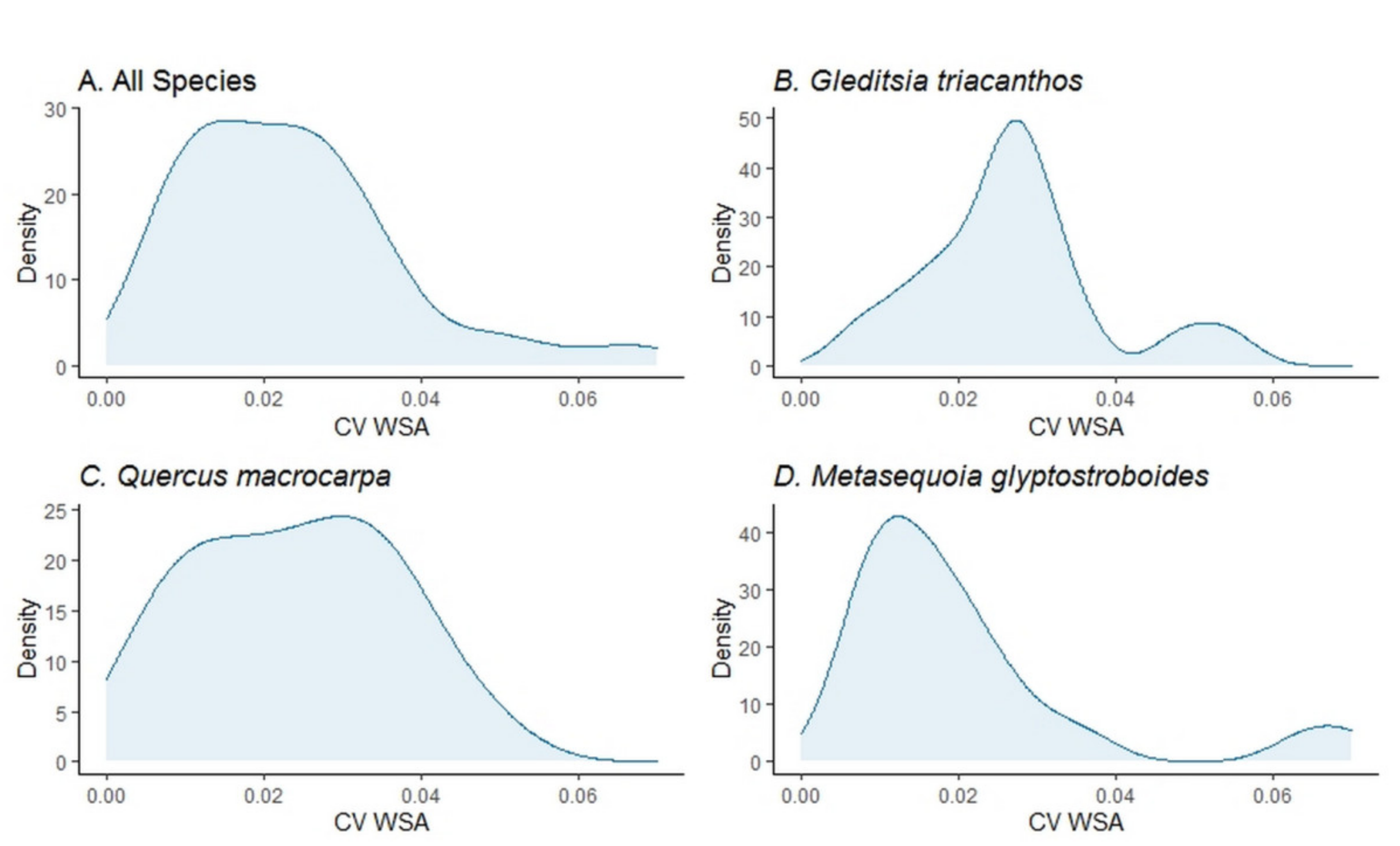
| CV WSA (mean [min, max]) | 0.024 [0.005, 0.07] | 0.027 [0.007, 0.054] | 0.024 [0.005, 0.047] | 0.021 [0.007, 0.07] |
| Stem WSA (m2) (mean [min, max]) | 12.5 [1.5, 44.6] | 11.3 [4.1, 20.1] | 16.2 [4.7, 30.3] | 11.0 [1.5, 44.6] |
| Branch WSA (m2) (mean [min, max]) | 186.8 [12.4, 436.7] | 256.3 [61.2, 395.5] | 209.2 [55.7, 436.7] | 117.9 [12.4, 352.9] |
| No. of branch orders (median [min, max]) | 5 [1, 11] | 5 [1, 11] | 5 [1, 10] | 4 [1, 9] |
| Db leaf.off (mean [min, max]) | 1.98 [1.82, 2.15] | 2.03 [1.84, 2.11] | 1.92 [1.82, 2.04] | 1.99 [1.84, 2.15] |
| Mean Path length (m) (mean [min, max]) | 12.4 [3.7, 23.9] | 14.6 [9.5, 22] | 14.0 [6.9, 23.9] | 9.8 [3.7, 23.8] |
| Min Path length (m) (mean [min, max]) | 3.4 [0.8, 7.9] | 4.5 [2.4, 7.0] | 3.7 [2.1, 7.0] | 2.3 [0.8, 7.9] |
| Max Path length (m) (mean [min, max]) | 22.1 [6.5, 44.0] | 24.5 [17.3, 37.5] | 24.9 [12.3, 42.7] | 18.5 [6.5, 44.0] |
| SD Path length (m) (mean [min, max]) | 3.1 [1, 6.9] | 2.8 [2, 5.1] | 3.6 [1.5, 6.1] | 2.9 [1, 6.9] |
| 25th % Path length (mean [min, max]) | 10.4 [2.9, 20.6] | 13 [7.7, 18.1] | 11.7 [5.4, 20.6] | 7.7 [2.9, 19.5] |
| 50th % Path length (mean [min, max]) | 12.5 [3.6, 24.5] | 14.6 [9.8, 23] | 14.1 [6.6, 24.1] | 9.7 [3.6, 24.5] |
| 75th % Path length (mean [min, max]) | 14.4 [4.4, 28.7] | 16.1 [11.4, 25.1] | 16.5 [8.3, 28.7] | 11.7 [4.4, 28] |
| Model | Adjusted R2 | AIC Values |
|---|---|---|
| WSA ~ Db + Mean L|spp. + ε | 0.856 | 599.02 |
| WSA ~ Db + 25th % L|spp. + ε | 0.863 | 595.49 |
| WSA ~ Db + 50th % L|spp. + ε | 0.855 | 599.78 |
| WSA ~ Db + 75th % L|spp. + ε | 0.852 | 601.38 |
Publisher’s Note: MDPI stays neutral with regard to jurisdictional claims in published maps and institutional affiliations. |
© 2021 by the authors. Licensee MDPI, Basel, Switzerland. This article is an open access article distributed under the terms and conditions of the Creative Commons Attribution (CC BY) license (https://creativecommons.org/licenses/by/4.0/).
Share and Cite
Arseniou, G.; MacFarlane, D.W.; Seidel, D. Woody Surface Area Measurements with Terrestrial Laser Scanning Relate to the Anatomical and Structural Complexity of Urban Trees. Remote Sens. 2021, 13, 3153. https://doi.org/10.3390/rs13163153
Arseniou G, MacFarlane DW, Seidel D. Woody Surface Area Measurements with Terrestrial Laser Scanning Relate to the Anatomical and Structural Complexity of Urban Trees. Remote Sensing. 2021; 13(16):3153. https://doi.org/10.3390/rs13163153
Chicago/Turabian StyleArseniou, Georgios, David W. MacFarlane, and Dominik Seidel. 2021. "Woody Surface Area Measurements with Terrestrial Laser Scanning Relate to the Anatomical and Structural Complexity of Urban Trees" Remote Sensing 13, no. 16: 3153. https://doi.org/10.3390/rs13163153