Article

Modeling Diameter Distributions with Six Probability Density Functions in Pinus halepensis Mill. Plantations Using Low-Density Airborne Laser Scanning Data in Aragón (Northeast Spain)

by
J. Javier Gorgoso-Varela
1,*,
Rafael Alonso Ponce
2,3 and
Francisco Rodríguez-Puerta
3,4
1
Campus de Lugo, University of Santiago de Compostela, 27002 Lugo, Spain
2
Campus Duques de Soria, Föra Forest Technologies SLL, 42004 Soria, Spain
3
Campus Duques de Soria, Sustainable Forest Management Research Institute UVa-INIA, 42004 Soria, Spain
4
Campus Duques de Soria, University of Valladolid, 42004 Soria, Spain
*
Author to whom correspondence should be addressed.
Remote Sens. 2021, 13(12), 2307; https://doi.org/10.3390/rs13122307
Submission received: 13 May 2021 / Revised: 7 June 2021 / Accepted: 9 June 2021 / Published: 12 June 2021
(This article belongs to the Special Issue Advances in LiDAR Remote Sensing for Forestry and Ecology)

Abstract

:
The diameter distributions of trees in 50 temporary sample plots (TSPs) established in Pinus halepensis Mill. stands were recovered from LiDAR metrics by using six probability density functions (PDFs): the Weibull (2P and 3P), Johnson’s SB, beta, generalized beta and gamma-2P functions. The parameters were recovered from the first and the second moments of the distributions (mean and variance, respectively) by using parameter recovery models (PRM). Linear models were used to predict both moments from LiDAR data. In recovering the functions, the location parameters of the distributions were predetermined as the minimum diameter inventoried, and scale parameters were established as the maximum diameters predicted from LiDAR metrics. The Kolmogorov–Smirnov (KS) statistic (Dn), number of acceptances by the KS test, the Cramér von Misses (W2) statistic, bias and mean square error (MSE) were used to evaluate the goodness of fits. The fits for the six recovered functions were compared with the fits to all measured data from 58 TSPs (LiDAR metrics could only be extracted from 50 of the plots). In the fitting phase, the location parameters were fixed at a suitable value determined according to the forestry literature (0.75·dmin). The linear models used to recover the two moments of the distributions and the maximum diameters determined from LiDAR data were accurate, with R2 values of 0.750, 0.724 and 0.873 for dg, dmed and dmax. Reasonable results were obtained with all six recovered functions. The goodness-of-fit statistics indicated that the beta function was the most accurate, followed by the generalized beta function. The Weibull-3P function provided the poorest fits and the Weibull-2P and Johnson’s SB also yielded poor fits to the data.

Graphical Abstract

1. Introduction

LiDAR (Laser Imaging Detection and Ranging) technology allows large areas to be scanned, thus generating continuous information about the entire space. In the last 20 years, LiDAR has been increasingly used in forest inventories at different scales [1,2], because of its ability to provide detailed three-dimensional information on the size and structure of forest cover [3]. The process provides data on the dimensions of the trees and on the structure of the forest cover, and other parameters such as canopy fuel attributes [4]. The variables most closely related to LiDAR data are canopy cover and tree height, which mainly depend on the vertical distribution of the layers forming the tree cover [5,6].
The main advantage of using field data that will then be processed using LiDAR techniques is that a much smaller sampling effort is required (with a good sampling design), regarding both the number of plots and the number of tree height measurements required. LiDAR technology, such as airborne laser scanning (ALS), provides a great deal of information about vegetation height and is usually quite accurate, especially in coniferous plantations. This technology therefore represents the future of forest inventories, especially on a large scale, greatly reducing the costs associated with inventories, which are traditionally the most expensive part of forest management projects.
One of the most common approaches used in ALS forest inventories is the area-based approach (ABA), in which metrics extracted from the normalized height of the LiDAR data cloud (NHD) are used to predict forest variables [7]. Although the ABA does not directly detect tree diameters, it determines the forest stand structure indirectly by using the NHD metrics to estimate probability density functions (PDF) that describe diameter distributions [6].
The empirical diameter distribution (specified by the DBH measurements within the stand) described by a cumulative distribution function (CDF) or a PDF enables prediction of stand growth and planning of various uses and provides data about stand structure. The diameter distribution of the total number of trees in a stand is important because the model parameters and stand variables provided in yield tables are closely related [8]. However, DBH measurements are not always available, and therefore the diameter distribution must be predicted by using stand attributes as explanatory variables, usually under the assumption that they can be described by a specified theoretical PDF [6,9].
However, the parameters of the PDFs can also be estimated from LiDAR metrics. Three approaches have been considered for estimating the diameter distribution from LiDAR data, within the framework of parametric prediction [6]: (a) use of regression analysis and parameter recovery models (PRM) to relate LiDAR metrics directly to PDF parameters or the moments or percentiles of the diameter distribution, (b) modeling the PDF parameters from stand-level variables predicted using area-based LiDAR metrics and (c) predicting the diameter distribution on the basis of recognition of individual trees, which requires high pulse densities. The first approach has recently been used, with good results [10,11], and is the methodology used in the present study.
Several CDFs or PDFs have been used to describe and predict tree diameter frequency in forest stands, including Gram-Charlier [12], normal [13], Birnbaum–Saunders, and gamma [14], beta [15], generalized beta [16], Johnson’s SB [17] and the Weibull [18] functions. To date, the parameters of these distributions have only been recovered from LiDAR metrics by applying PRM to the Weibull distribution [10,19,20] and Johnson’s SB distribution [11]. However, this approach has never been used with distributions such as the beta, generalized beta and gamma-2P functions.
Thus, the main objective of this study was to predict and to compare the diameter distributions in Pinus halepensis Mill. plantations in Aragón (NE Spain) recovered by PRM in combination with the Weibull (2P and 3P), Johnson’s SB, beta, generalized beta and gamma-2P functions, and using height and canopy cover LiDAR metrics from low-density airborne scanning data provided by the Spanish country-wide PNOA (Plan Nacional de Ortografía Aérea), which covers the whole country, so our study can be scalable to other species using the same methodology and type of data.

2. Materials and Methods
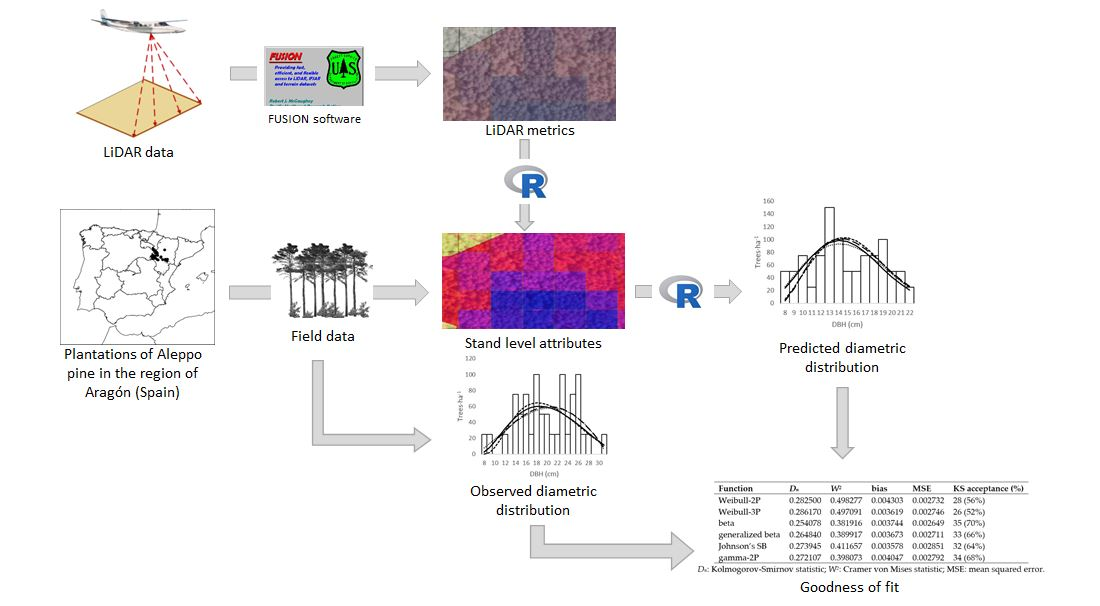
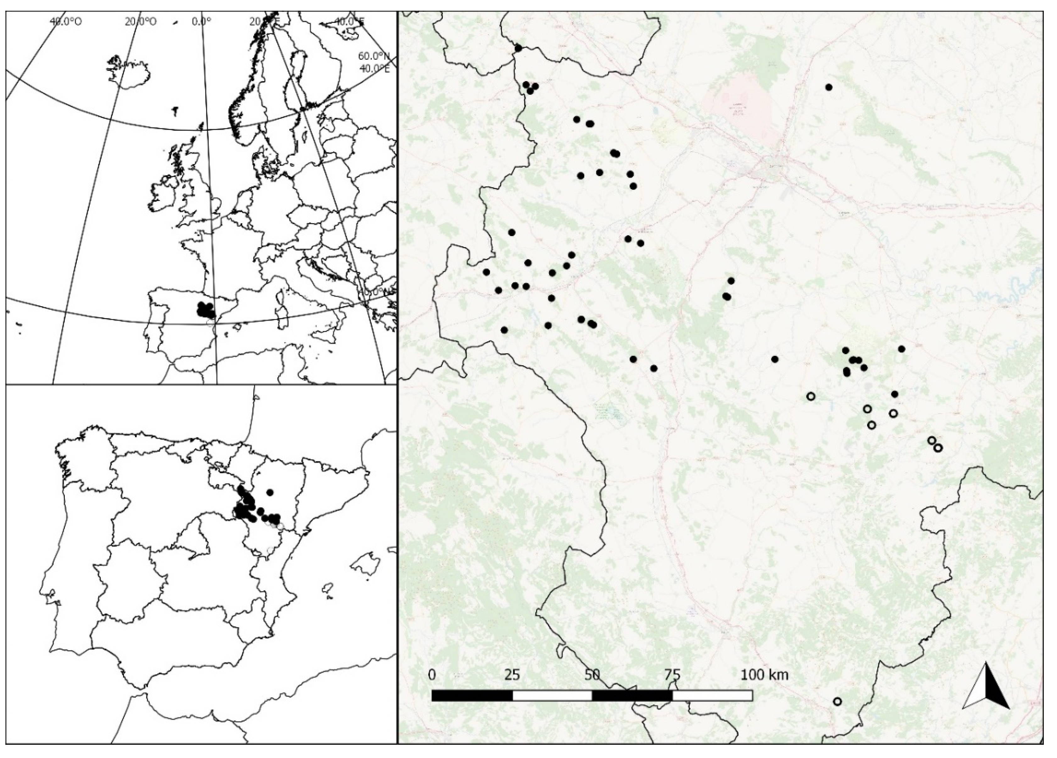
2.1. Dataset

The data used in this study were obtained from plantations of Aleppo pine (Pinus halepensis Mill.) in the region of Aragón (NE Spain). P. halepensis is distributed naturally throughout the Mediterranean area of the southeast of the Iberian Peninsula and the Balearic Islands [21]. Plantations of the species represent 15% of those established between 1940 and 1980 in Spain. However, the species is not particularly productive relative to other pines. Scant attention has therefore been given to Aleppo pine, even though at local scales it may be the only economic alternative available and may complement other non-timber harvests [22].
A total of 58 temporary sampling plots (TSPs) of P. halepensis Mill., measured in October 2017, were used for the present study, and LiDAR metrics were able to be extracted from the data corresponding to 50 of these plots (Figure 1). The plot size ranged from 225 to 625 m2, to achieve a minimum number of 30 trees per plot. Diameter at breast height (DBH at 1.3 m above the ground) of a total of 1685 trees was measured with callipers, to an accuracy of 0.1 cm. The following field and LiDAR variables were calculated from the inventory data: quadratic mean diameter, mean diameter, maximum diameter, number of trees per hectare, dominant height, basal area and total LiDAR return density within the plots (pulses·m−2). Summary statistics are shown in Table 1.

2.2. Lidar Metrics

The LiDAR data covering 50 plots in Pinus halepensis stands were acquired in a national survey carried out for the PNOA (Plan Nacional de Ortofotografía de España) project between 16 October and 16 November 2016, under the direction of the Spanish Ministerio de Fomento (Dirección General del Instituto Geográfico Nacional and Centro Nacional de Información Geográfica). The data were obtained with a LEICA ALS80 sensor, at a pulse repetition rate of 45 kHz, scan frequency of 70 Hz and a maximum scan angle of ±50°. A maximum of 4 returns per pulse were registered, reaching an average point density of 1.070 points·m−2, with a theoretical laser pulse density required for the PNOA project of 0.5 first returns per square meter. Summary statistics of the LiDAR return density per square meter within the plots are shown in Table 1. The LiDAR data were also processed with FUSION software [23]. As reported by the provider (https://pnoa.ign.es/) accessed on 1 April 2020, the vertical accuracy of the LiDAR metrics, given by the RMSE, is ≤0.20 m. The set of metrics from the points laid above 2 m was extracted for each plot (Table 2).

2.3. Diameter Distribution Models and Fitting

2.3.1. The Weibull Function

The three-parameter Weibull PDF has the following expression for a continuous random variable x [24]:
f ( x ) = ( c b ) · ( x a b ) c 1 · e ( x a b ) c
where f(x) is the probability density of trees with diameter x, a represents the location, b the scale and c the shape. If a equals zero, the expression corresponds to the two-parameter Weibull function.
The method of moments was used to fit all six distributions on the basis of the relationship between the parameters and the first and second moments of the diameter distribution (arithmetic mean diameter and variance). For the Weibull distribution, it is computed by the following expressions [10,18]:
b = d ¯ a Γ ( 1 + 1 c )
σ 2 = ( d ¯ a ) 2 Γ 2 ( 1 + 1 c ) [ Γ ( 1 + 2 c ) Γ 2 ( 1 + 1 c ) ]
where d ¯ is the arithmetic mean diameter of the distribution, σ 2 is the variance and Γ ( · ) is the gamma function. Equation (3) was resolved by a bisection iterative procedure [25].

2.3.2. The Beta Function

The general expression of the beta distribution for a random variable x is given by [26]:
f ( x ) = c · ( x L ) · ( U x ) γ
w i t h   c = 1 ( L + U ) 1 + γ · Γ ( 1 + α ) · Γ ( 1 + γ ) ( 1 L + U ) α · Γ ( 2 + α + γ )  
for the interval L ≤ x ≤ U, and x = 0 otherwise, where x is the diameter at breast height and is assumed to be continuous, f(x) is the density associated with diameter x, U and L are respectively the upper and lower limits of the beta distribution, c is the scaling factor, α and γ are respectively the first and the second exponents that determine the shape of the distribution and Γ ( · ) is the gamma function.
The method of moments for the beta function [9,15,27] is computed by the following equations:
γ = Z s r e l 2 · ( Z + 1 ) 2 1 Z + 1 1  
α = Z · ( γ + 1 ) 1
Z = x r e l 1 x r e l  
x r e l = d ¯ L U L
s r e l 2 = s 2 ( U L ) 2 .
where d ¯ is the arithmetic mean diameter of the distribution and s 2 is the variance.

2.3.3. The Generalized Beta Distribution (GBD)

The general expression of the generalized beta PDF for a random variable x is as follows [16]:
f ( x ) = · β 2 ( β 3 + β 4 + 1 ) · ( x β 1 ) β 3 · ( β 1 + β 2 x ) β 4
w h e r e   = Γ ( β 3 + β 4 + 2 ) Γ ( β 3 + 1 ) · Γ ( β 4 + 1 )
for the interval ( β 1 ,   β 1 + β 2 ) , and 0 otherwise, where x is the diameter at breast height and is assumed to be continuous, f(x) is the density associated with diameter x, β 1 and β 2 are respectively the lower and upper limits of the distribution, β 3 and β 4 are exponents that determine the shape of the distribution, is the scaling factor of the function and Γ ( · ) is the gamma function.
The method of moments for the GBD function is computed by the following expressions [16,28]:
β 1 = x m i n   β 3 = ( α 1 β 1 ) 2 ( β 1 + β 2 α 1 ) α 2 ( β 2 β 1 + α 1 ) α 2 β 2
β 2 = x m a x β 1   β 4 = β 2 ( β 3 + 1 ) α 1 β 1 β 3 2
where x is the tree diameter, α 1 is the arithmetic mean diameter and α 2 is the variance.

2.3.4. The Johnson’s SB Function

The model of the Johnson’s SB PDF has the following expression for a continuous random variable x [29]:
f ( x ) = δ 2 π · λ ( ε + λ x ) ( x ε ) · e 1 2 [ γ + δ · l n ( x ε ε + λ x ) ] 2
where f(x) is the probability density associated with diameter x, ε < x < ε + λ, ∞ < ε < , ∞ < γ < , λ > 0, and δ > 0.
The model is characterized by the parameters ε (location), λ (scale), γ (asymmetry) and δ (kurtosis). The method of moments used in [11,30] is computed as follows:
δ μ ( 1 μ ) S d ( x ) + S d ( x ) 4 [ 1 μ ( 1 μ ) 8 ]  
γ δ l n ( 1 μ μ ) + ( 0.5 μ δ )
μ = d ¯ ε λ
S d ( x ) = σ x λ  
where d ¯ is the arithmetic mean of the plot diameters, Sd(x) is the modified standard (δ) deviation and σ x is the plot diameter standard deviation.

2.3.5. The Gamma Function

The model of the gamma PDF has the following expression for a continuous random variable x [14,31]:
f ( x ) = ( x γ ) α 1 β α Γ ( α ) · e [ ( x γ β ) ]
with x > γ , α > 0 and β > 0, where α is the shape parameter, β is an inverse scale parameter, γ is the location parameter ( γ = 0 for the two-parameter gamma distribution) and Γ ( · ) is the gamma function.
The method of moments for the gamma-2P function is computed by the following expressions [28]:
α = ( d ¯ s ) 2
β = s 2 d ¯  
where d ¯ is the mean diameter and s is the standard deviation.
For fitting the distributions to the observed data (phase 1), a value of 0.75·dmin was used for the location parameters, as [32] achieved good results with this value compared to other constraints. For the Weibull-2P and gamma-2P functions, the value of the location parameters was zero. Scale parameters and the upper limit of the four-parameter functions (Johnson’s SB, beta and generalized beta) were established as the maximum diameter of the distributions (dmax) and the upper limit of the largest diameter class for the beta function [27,28] to improve parameters’ convergence. The size of the diameter classes was assumed to equal 1 cm.

2.4. Goodness of Fit Evaluation

The consistency of the functions was evaluated using the Kolmogorov–Smirnov (KS) (Dn) and Cramér von Mises (W2) statistics, bias, mean square error (MSE) and number of acceptances by the KS test. For a given cumulative distribution function, F(x), D n = s u p x | F n ( x ) F 0 ( x ) | , where supx is the supremum of the set of distances, calculated as follows [33]:
D n = m a x { m a x 1 i n i [ F n ( x i ) F 0 ( x j ) ] ,   m a x 1 i n i [ F 0 ( x j ) F n ( x i 1 ) ] }
where the cumulative observed and estimated frequencies, i.e., Fn(xi) and F0(xj), are compared.
The recovered distributions were also assessed using the two-sample Kolmogorov–Smirnov test (KS) under the null hypothesis that the plot data originate from the recovered distribution. However, as the parameters were estimated empirically, the theoretical distribution for each plot is unknown, and the KS test should therefore be conducted using a Monte Carlo simulation [34]. The procedure is explained in further detail in [10,11].
The Cramér von Mises statistic (W2) is a measure of the square of the distance between the empirical and the cumulative theoretical distribution [35]:
W 2 = i = 1 n { F ^ ( x i ) ( i 0.5 ) n } 2 + 1 12 n
where F ^ ( x i ) is the cumulative theoretical distribution in diameter class i, and n is the number of diameter classes.
The bias and the mean square error (MSE) were also used as goodness-of-fit measures and were expressed as follows:
B i a s = i = 1 N Y i Y ^ i N
M S E = i = 1 N ( Y i Y ^ i ) 2 N
where Yi is the observed relative frequency of trees in each diameter class, Y i ^ is the theoretical value predicted by the model and N is the number of diameter classes. The bias and MSE were calculated for each fit as the mean relative frequency of trees.

2.5. Recovering the Parameters of the Distributions from LiDAR Metrics
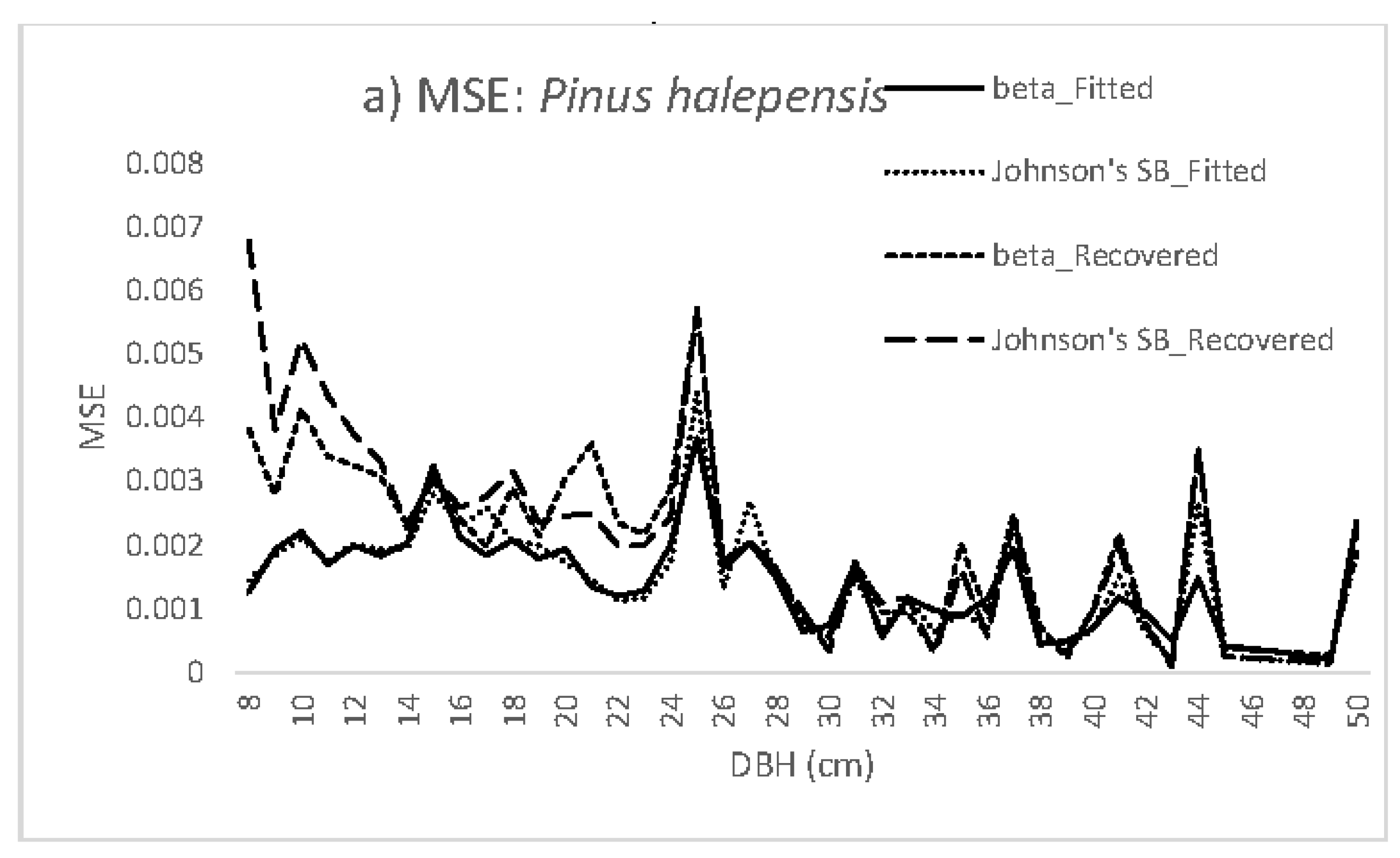
The function parameters were recovered from the first two moments of the distributions (mean diameter and variance) by using parameter recovery models (PRMs). The variance ( σ d 2 ) is related to the quadratic mean diameter (dg) and the mean diameter (dm), as follows:
σ d 2 = d g 2 d m 2
Within the LiDAR data framework, the stand level attributes usually used for the recovery procedure (e.g., t, N, H, S) can be replaced by LiDAR metrics as explanatory variables to estimate dg and dm [10]. However, in the four-parameter functions (Johnson’s SB, beta and generalized beta), the range and the upper limit of the distributions can also be estimated. In this case, both values were used as the maximum diameter (dmax), which was then related to LiDAR metrics. Location parameters of the recovered functions were predetermined as the minimum diameter inventory (7.5 cm) for the Weibull-3P, Johnson’s SB, beta and generalized beta functions, and as zero for the Weibull-2P and gamma-2P functions.
We used linear models to establish the empirical relationships between dmax, dg and LiDAR metrics:
d m a x = α 0 + α 1 X 1 + α 2 X 2 + + α m X m + ε
d g = β 0 + β 1 X 1 + β 2 X 2 + + β m X m + ε
where dmax and dg are the dependent variables, X1, X2, …, Xm represents the independent, potentially explanatory variables related to the LiDAR-derived height distribution and canopy closure, α 0 , α 1 , … α n and β 0 , β 1 , … β n are the parameters to be estimated in the fitting process and ε is the additive error term, which is assumed to be independent and normally and identically distributed, with zero mean.
For a given stand, dm is always smaller than or equal to dg, and we therefore used the following model expression to take this restriction into account [9,10,11,36]:
d m = d g exp ( δ 0 + δ 1 X 1 + δ 2 X 2 + + δ m X m ) + ε
where X1, X2, …, Xm are the potential explanatory variables related to the LiDAR-derived height distribution and canopy closure, δ 0 , δ 1 ,… δ m are the parameters to be estimated in the fitting process and ε is the additive error term.
Equation (30) was linearized by applying a natural logarithmic transformation to facilitate selection of the independent variables. Finally, Equation (29) (when dg was the dependent variable) and Equation (30) were fitted simultaneously with “seemingly unrelated regression” (SUR) to prevent cross-correlation between error components. Goodness of fits were evaluated with the coefficient of determination (R2) and the root mean square error (RMSE).

3. Results

The mean, standard deviation, minimum and maximum values of the parameters estimated in step 1 (fitting the distributions to observed data) and step 2 (recovering the parameters of the distributions from LiDAR metrics) are shown in Table 3.
The mean values of the parameters were reasonable in both cases, with no large differences in the values produced by each method. Table 4 shows the mean value of the statistics used to test the goodness-of-fits to the observed distributions: Kolmogorov–Smirnov (Dn), Cramér von Mises (W2), bias and mean squared error (MSE).
In the fitting phase, the lowest value of Dn was yielded by the beta function (0.138560), followed by the Weibull-2P function (0.146922) and the Weibull-3P function (0.150761). The highest value was yielded by the gamma-2P function (0.164750), followed by the Johnson’s SB function (0.162578) and the generalized beta function (0.153656). Regarding the Cramér von Mises statistic (W2), the lowest value corresponded to the Johnson’s SB function (0.043088) and the highest to the Weibull-2P function (0.081863). The order of the functions in terms of W2 was Johnson’s SB < Weibull-3P < generalized beta < gamma-2P < beta < Weibull-2P. The smallest MSE value corresponded to the beta function (0.001851), followed by the generalized beta function (0.001879). The highest MSE value was yielded by the Weibull-2P function (0.002009). The order for the six distributions studied was beta < generalized beta < Johnson’s SB < Weibull-3P < gamma-2P < Weibull-2P. The bias may be less important for comparison of the results because errors with different signs can compensate each other in the total mean value. Thus, considering the values of Dn, W2 and MSE for the six distributions studied, the beta function provided the most accurate fits to the observed data and the Weibull-2P and the Gamma-2P functions yielded the poorest fits.
The parameter estimates and goodness-of-fit statistics (R2, RMSE and % RMSE) of the simultaneous fitting of Equations (29) and (30) used to estimate the mean diameter (dm) and the quadratic mean diameter (dg) from LiDAR data and for Equation (28) used to estimate dmax are shown in Table 5.
The maximum diameter of the distributions (dmax) was considered the scale parameter for the Weibull-3P, Johnson’s SB and generalized beta functions and for establishing the upper limit of the beta function. The maximum diameter was predicted by the following independent variables: mean absolute deviation for height (LH_AAD) and 95% height percentile (LH_P95). The linear model yielded an accuracy of R2 = 0.873 and RMSE = 2.758. Models [29,30] used for simultaneous fitting of quadratic mean diameter (dg) and the mean diameter (dmed) yielded R2 values of 0.750 and 0.724 and RMSE values of 2.542 and 2.549, respectively. Good results were obtained for these key variables in terms of recovering the diameter distributions with the six functions.
For recovering the distributions from LiDAR data (Table 6), the smallest value of Dn was obtained by the beta function (0.254078), as in the fitting step, and then by the generalized beta function (0.264840) and the gamma-2P function (0.272107). The highest value was yielded by the Weibull-3P function (0.286170), followed by the Weibull-2P function (0.282500) and the Johnson’s SB function (0.273945).
The lowest value of the Cramér von Mises statistic (W2) was also yielded by the beta function (0.381916) and the highest by the Weibull-2P function (0.498277). The order of the distributions for the W2 value was beta < generalized beta < gamma-2P < Johnson’s SB < Weibull-3P < Weibull-2P. As for Dn and W2, the smallest value for the MSE corresponded to the beta distribution (0.002649), followed by the generalized beta function (0.002711). The highest value of the MSE corresponded to the gamma-2P function (0.002792). The order in terms of MSE for the six distributions recovered was beta < generalized beta < Weibull-2P < Weibull-3P < gamma-2P < Johnson’s SB. As for the other statistics, bias was also higher for recovery of the distributions from LiDAR metrics than for fitting to the observed data. Results for the KS test are also consistent with the other statistics, with the following order for plots accepted: beta function (35 plots: 70%), gamma-2P function (34 plots: 68%), generalized beta function (33 plots: 66%), Johnson’s SB function (32 plots: 64%), Weibull-2P function (28 plots: 56%) and Weibull-3P function (26 plots: 52%). Thus, considering the values of Dn, W2, MSE and KS test for the six distributions studied, the beta function was the most accurate for recovering the parameters from LiDAR data, followed by the generalized beta function. The Weibull-3P, Weibull-2P and the Johnson’s SB functions yielded poorer results.
The mean values of the MSE in each diameter class for the fits to the observed data and for recovering from LiDAR data for the best (beta) and the poorest (Johnson’s SB) functions are shown in Figure 2a, while those for the generalized beta vs. Weibull-3P and for the gamma-2P vs. Weibull-2P functions are also shown in Figure 2b,c. Figure 2a shows that the MSE for the fits to the observed data was almost the same for both functions (beta and Johnson’s SB) over the diameter range studied, decreasing when the diameters increased. However, significant differences were observed for recovery of the functions. The recovered distributions yielded much larger values of MSE, up to 25 cm, after which both values (fitted and recovered) were more similar. The recovered Johnson’s SB yielded the largest values up to 19 cm, while the beta function was less accurate at between 19 and 24 cm. The difference between fitting and recovery of the smallest diameter classes increased with the number of data points.
Figure 2b shows the same trends for the range studied, with similar behavior obtained for fitting and recovery of both the generalized and Weibull-3P distributions. Figure 2c shows similar results produced by the gamma-2P and Weibull-3P functions.
Graphical assessment of the observed, described (fitted) and recovered distributions for six plots fits are shown in Figure 3. Pairwise comparisons of the functions were made: beta vs. Johnson’s SB (Figure 3a), generalized beta vs. Weibull-3P (Figure 3b) and gamma-2P vs. Weibull-2P (Figure 3c). The predictions were reasonable and followed the observed diameter distributions, especially for plots 1, 3, 4 and 6.

4. Discussion

We used a total of 58 TSPs from P. halepensis Mill. plantations for the present study, and LiDAR metrics were able be extracted from 50 of these plots. The number of plots is greater than in other studies of diameter distributions recovered from LiDAR data in the Northwest Iberian Peninsula [10,11]. These studies recovered the Weibull-2P and the Johnson’s SB distributions from LiDAR metrics. The Weibull function (2P and 3P) is the most commonly used distribution in this type of study [20,37,38]. However, in the present study, we used, for the first time within the framework of LiDAR-based research, three functions commonly used to describe and predict diameter distributions in forest stands, i.e., the beta [26], generalized beta [16] and gamma-2P [14] functions. In some cases, the results obtained were better than those obtained with the more usual Weibull (2P and 3P) and Johnson’s SB functions, for both fitting to the observed data and recovering with LiDAR metrics.
For the fitting phase, the results obtained for the main statistics used (Dn, W2 and MSE) are similar to those obtained in [28] for Eucalyptus globulus stands in NW Spain. However, more accurate results were obtained in the same study for Pinus radiata stands by using the same functions. In a previous study, similar results were also obtained for Pinus sylvestris and better than those reported for Pinus pinaster stands in NW Spain [32].
The models used to recover the parameters of the distributions from moments of the distributions were accurate. Explanatory variables were LH_P90 (height percentile of 90%) for dg, and LH_MAD_MEDIAN (median of the absolute deviations from the overall height median) for dmed. In other studies, height percentiles were also used as independent variables for estimating dg (75% percentile and number of LiDAR last returns above a height of 1 m) and for dmed (1% percentile) in the models obtained in [10] for recovering the Weibull-2P distribution in 25 plantation plots of Pinus radiata in Northwest Spain, with R2 for the dg and dmed models of 0.80 and 0.77, respectively. For Pinus halepensis, we obtained similar R2 values (0.75 and 0.72 for dg and dmed, respectively). The RMSE values (2.54 cm for dg and 2.55 cm for dmed) are consistent with the values reported in international forestry literature. For example, for German forests dominated by Picea abies (L.) Karst., the authors of [39] used data from a 0.44 pulse m−2 LiDAR flight and reported an RMSE of 2.44 cm for dmed, while the authors of [40] studied a broad range of forest types (coniferous and hardwoods) and conditions across Ontario by using an artificially reduced LiDAR database of 0.5 pulses m−2, reporting RMSE values ranging from 0.76 to 4.3 cm for dg. The authors of [10] reported RMSE values of 3.42 for dg and 3.63 for dmed, while the authors of [11] used exponential models instead of linear models to estimate the moments of the Johnson’s SB and the Weibull-2P functions, obtaining an R2 of 0.82 and 0.86 for the dmed of Pinus radiata and Eucalyptus globulus respectively, and 0.84 and 0.89 for dg of the same species. We compared the use of linear and exponential models for obtaining both variables and found that the results were similar, with the exponential model even including more independent variables. Thus, the linear models were considered more suitable.
Use of the four-parameter Johnson’s SB, beta and generalized beta distributions requires knowledge about the location parameter of the three distributions, the scale for the Johnson’s SB and the upper limit of the distributions for the beta and generalized beta functions. The three-parameter Weibull-3P requires knowledge about the location parameter, while in the Weibull-2P and gamma-2P functions, the value of the location parameter is zero. In functions with a location parameter, the value considered in the recovery phase with LiDAR metrics was the minimum diameter inventory (7.5 cm). This avoided having to model this parameter with LiDAR metrics, which can produce inaccurate results if stand variables are used in the model [9]. Thus, in all cases, the location parameter was considered equal to 7.5 cm for recovering the distributions from LiDAR data, while for fitting to the observed data, it was assumed to be 0.75·dmin, producing a similar mean value considering all plots of 7.18 cm (Table 3). The authors of [11] considered the location parameter for the Johnson’s SB to equal zero, thus avoiding modeling it with LiDAR metrics, while the scale parameter considered was also the maximum diameter (dmax).
The model obtained for dmax included, as LiDAR explanatory variables, LH_AAD (mean absolute deviation for height) and LH_P95 (95% height percentile), with R2 = 0.87 and % RMSE = 10.56. The authors of [11] obtained similar values for Pinus radiata (R2 = 0.93 and % RMSE = 8%) and Eucalyptus globulus (R2 = 0.83 and % RMSE = 12%). The results for this variable modeled from LiDAR data are more accurate than those obtained in [27] and [9] with stand variables. The statistics obtained for recovery of the six functions were also reasonable. For example, the authors of [32] reported Dn values of 0.1924 for the Weibull-2P fitted by Maximum Likelihood, 0.2285 for the Johnson’s SB fitted by conditional maximum likelihood (CML) and 0.1812 for the beta fitted by moments to observed distributions of Pinus pinaster in Northwest Spain. The authors of [33] obtained a Dn value of 0.193 in the fits by maximum likelihood of the Weibull-3P to observed data of Pinus taeda plantations in the USA. The value obtained for the recovered beta from LiDAR metrics (0.2541) is close to these values. The number of KS acceptances are consistent with those found in previous studies. The percentage of acceptance (between 52% and 70%) was similar for Eucalyptus globulus in northwest Portugal [11] and higher than in Pinus radiata stands in northwest Spain [10,11].

5. Conclusions

Scant attention has been given to Aleppo pine plantations in Spain. However, we recovered the parameters of six probability density functions, i.e., the Weibull (2P and 3P), Johnson’s SB, beta, generalized beta and gamma-2P functions, from LiDAR metrics in 50 Pinus halepensis stands in Aragón (northeast Spain). The beta, generalized beta and gamma- 2P functions are of novel application in the field of LiDAR-based research. The results obtained were reasonable compared with previous studies and they showed that the beta and generalized beta functions were more accurate than the Johnson’s SB and Weibull (2P and 3P) functions, which are more commonly used in this type of study. None of the distributions predicted anomalous results.

Author Contributions

Conceptualization, J.J.G.-V.; methodology, J.J.G.-V.; software, J.J.G.-V. and R.A.P.; validation, J.J.G.-V.; formal analysis, J.J.G.-V. and R.A.P.; investigation, J.J.G.-V., R.A.P. and F.R.-P.; resources, R.A.P. and F.R.-P.; data curation, J.J.G.-V., R.A.P. and F.R.-P.; writing—original draft preparation, J.J.G.-V.; writing—review and editing, J.J.G.-V.; visualization, J.J.G.-V. and F.R.-P.; supervision, J.J.G.-V.; project administration, R.A.P. and F.R.-P.; funding acquisition, R.A.P. and F.R.-P. All authors have read and agreed to the published version of the manuscript.

Funding

This work was supported by the Government of Spain, Department of Economy, Industry and Competitiveness, under a Torres Quevedo Contract PTQ-16-08445. This study was also supported by FEADER under the provisions of the Rural Development Program of Aragón 2014-2020 for the project RF-64079.

Conflicts of Interest

The authors declare no conflict of interest. The funders had no role in the design of the study; in the collection, analyses, or interpretation of data; in the writing of the manuscript, or in the decision to publish the results.

References

  1. Chen, W.; Hu, X.; Chen, W.; Hong, Y.; Yang, M. Airborne LiDAR Remote Sensing for Individual Tree Forest Inventory Using Trunk Detection-Aided Mean Shift Clustering Techniques. Remote Sens. 2018, 10, 1078. [Google Scholar] [CrossRef] [Green Version]
  2. Corte, A.P.D.; Souza, D.V.; Rex, F.E.; Sanquetta, C.R.; Mohan, M.; Silva, C.A.; Almeyda Zambrano, A.M.; Prata, G.; Alves de Almeida, D.R.; Trautenmüller, J.W.; et al. Forest inventory with high-density UAV-Lidar: Machine learning approaches for predicting individual tree attributes. Comput. Electron. Agric. 2020, 179, 105815. [Google Scholar] [CrossRef]
  3. Wagner, W.; Hollaus, M.; Briese, C.; Ducic, V. 3D vegetation mapping using small-footprint full-waveform airborne laser scanners. Int. J. Remote Sens. 2008, 29, 1433–1452. [Google Scholar] [CrossRef] [Green Version]
  4. Engelstand, P.S.; Falkowski, M.; Wolter, P.; Poznanovic, A.; Johnson, P. Estimating Canopy Fuel Attributes from Low-Density LiDAR. Fire 2019, 2, 38. [Google Scholar] [CrossRef] [Green Version]
  5. Kotivuori, E.; Kukkonen, M.; Mehtätalo, L.; Maltamo, M.; Korhonen, L.; Packalen, P. Forest inventories for small areas using drone imagery without in-situ field measurements. Remote Sens. Environ. 2020, 237, 111404. [Google Scholar] [CrossRef]
  6. Maltamo, M.; Gobakken, T. Predicting tree diameter distributions. In Forestry Applications of Airborne Laser Scanning: Concepts and Cases Studies; Maltamo, M., Næsset, E., Vauhkonen, J., Eds.; Springer: Dordrecht, The Netherlands, 2014; pp. 269–292. [Google Scholar]
  7. Næsset, E. Predicting forest stand characteristics with airborne scanning laser using a practical two-stage procedure and field data. Remote Sens. Environ. 2002, 80, 88–99. [Google Scholar] [CrossRef]
  8. Gorgoso, J.J.; Alvarez-Gonzalez, J.G.; Rojo, A.; Grandas-Arias, J.A. Modelling diameter distributions of Betula alba L. stands in northwest Spain with the two-parameter Weibull function. For. Syst. 2007, 16, 113–123. [Google Scholar] [CrossRef] [Green Version]
  9. Gorgoso-Varela, J.J.; Rojo-Alboreca, A.; Afif-Khouri, E.; Barrio-Anta, M. Modelling diameter distributions of birch (Betula alba L.) and pedunculate oak (Quercus robur L.) stands in northwest Spain with the beta distribution. Invest. Agrar. Sist. Recur. For. 2008, 17, 271–281. [Google Scholar] [CrossRef] [Green Version]
  10. Arias-Rodil, M.; Diéguez-Aranda, U.; Álvarez-González, J.G.; Pérez-Cruzado, C.; Castedo-Dorado, F.; González-Ferreiro, E. Modeling diameter distributions in radiata pine plantations in Spain with existing countrywide LiDAR data. Ann. For. Sci. 2018, 75, 36. [Google Scholar] [CrossRef] [Green Version]
  11. Cosenza, D.N.; Soares, P.; Guerra-Hernández, J.; Pereira, L.; González-Ferreiro, E.; Castedo-Dorado, F.; Tomé, M. Comparing Johnson’s SB and Weibull Functions to Model the Diameter Distribution of Forest Plantations through ALS data. Remote Sens. 2019, 11, 2792. [Google Scholar] [CrossRef] [Green Version]
  12. Schnur, G.L. Diameter distributions for old-field loblolly pine stands in Maryland. J. Agric. Res. 1934, 49, 731–743. [Google Scholar]
  13. Sghaier, T.; Cañellas, I.; Calama, R.; Sánchez-González, M. Modelling diameter distribution of Tetraclinis articulata in Tunisia using normal and Weibull distributions with parameters depending on stand variables. iForest 2016, 9, 702–709. [Google Scholar] [CrossRef]
  14. Podlaski, R. Characterization of diameter distribution data in near-natural forests using the Birnbaum–Saunders distribution. Can. J. For. Res. 2008, 38, 518–527. [Google Scholar] [CrossRef]
  15. Palahí, M.; Pukkala, T.; Blasco, E.; Trasobares, A. Comparison of beta, Johnson’s SB, Weibull and truncated Weibull functions for modeling the diameter distribution of forest stands in Catalonia (north-east of Spain). Eur. J. For. Res. 2007, 126, 563–571. [Google Scholar] [CrossRef]
  16. Li, F.; Zhang, L.; Davis, C.J. Modeling the joint distribution of tree diameters and heights by bivariate generalized Beta distribution. For. Sci. 2002, 48, 47–58. [Google Scholar]
  17. Mateus, A.; Tomé, M. Modelling the diameter distribution of eucalyptus plantations with Johnson’s SB probability density function: Parameters recovery from a compatible system of equations to predict stand variables. Ann. For. Sci. 2011, 68, 325–335. [Google Scholar] [CrossRef] [Green Version]
  18. Pogoda, P.; Ochał, W.; Orzeł, S. Modeling Diameter Distribution of Black Alder (Alnus glutinosa (L.) Gaertn.) Stands in Poland. Forests 2019, 10, 412. [Google Scholar] [CrossRef] [Green Version]
  19. Gobakken, T.; Næsset, E. Estimation of diameter and basal area distributions in coniferous forest by means of airborne laser scanner data. Scand. J. For. Res. 2004, 19, 529–542. [Google Scholar] [CrossRef]
  20. Gobakken, T.; Næsset, E. Weibull and percentile models for lidar-based estimation of basal area distribution. Scand. J. For. Res. 2005, 20, 490–502. [Google Scholar] [CrossRef]
  21. Del Río, M.; Calama, R.; Montero, G. Selvicultura de Pinus halepensis Mill. In Compendio de Selvicultura Aplicada en España; Serrada, R., Montero, G., Reque, J.A., Eds.; Instituto Nacional de Investigación y Tecnología Agraria y Alimentaria: Madrid, España, 2008; pp. 289–312. [Google Scholar]
  22. Rojo-Alboreca, A.; Cabanillas-Saldaña, A.M.; Barrio-Anta, M.; Notivol-Paíno, E.; Gorgoso-Varela, J.J. Site index curves for natural Aleppo pine forests in the central Ebro Valley (Spain). Madera Bosques 2017, 23, 143–159. [Google Scholar] [CrossRef]
  23. McGaughey, R.J. FUSION/LDV: Software for LIDAR Data Analysis and Visualization. Version 3.50. USDA Forest Service—Pacific Northwest Research Station. 2015. Available online: http://forsys.cfr.washington.edu/fusion/fusionlatest.html (accessed on 31 January 2016).
  24. Bailey, R.L.; Dell, T.R. Quantifying Diameter Distributions with the Weibull Function. For. Sci. 1973, 19, 97–104. [Google Scholar]
  25. Gerald, C.F.; Wheatley, P.O. Applied Numerical Analysis, 4th ed.; Addison-Wesley Publishing Co.: Reading, MA, USA, 1989. [Google Scholar]
  26. Loetsch, F.; Zöhrer, F.; Haller, K.E. Forest Inventory 2; Verlagsgesellschaft. BLV: Munich, Germany, 1973; 469p. [Google Scholar]
  27. Maltamo, M.; Puumalaine, J.; Päivinen, R. Comparison of beta and Weibull functions for modelling basal area diameter distribution in stands of Pinus sylvestris and Picea abies. Scan. J. For. Res. 1995, 10, 284–295. [Google Scholar] [CrossRef]
  28. Gorgoso-Varela, J.J.; Ogana, F.N.; Ige, P.O. A comparison between derivative and numerical optimization methods used for diameter distribution estimation. Scand. J. For. Res. 2020, 35, 156–164. [Google Scholar] [CrossRef]
  29. Johnson, N.L. Systems of frequency curves generated by methods of translation. Biometrika 1949, 36, 149–176. [Google Scholar] [CrossRef]
  30. Scolforo, J.R.S.; Thierschi, A. Estimativas e testes da distribuição de frequência diâmétrica para Eucalyptus camaldulensis, através da distribuição SB, por diferentes métodos de ajuste. Sci. For. 1998, 54, 91–103. [Google Scholar]
  31. Nelson, T.C. Diameter distribution and growth of loblolly pine. For. Sci. 1964, 10, 105–115. [Google Scholar]
  32. Gorgoso, J.J.; Rojo, A.; Cámara-Obregón, A.; Diéguez-Aranda, U. A comparison of estimation methods for fitting Weibull, Johnson’s SB and beta functions to Pinus pinaster, Pinus radiata and Pinus sylvestris stands in northwest Spain. For. Syst. 2012, 21, 446–459. [Google Scholar] [CrossRef] [Green Version]
  33. Cao, Q. Predicting parameters of a Weibull function for modeling diameter distribution. For. Sci. 2004, 50, 682–685. [Google Scholar] [CrossRef]
  34. Lilliefors, H.W. On the Kolmogorov-Smirnov test for normality with mean and variance unknown. J. Am. Stat. Assoc. 1967, 62, 399–402. [Google Scholar] [CrossRef]
  35. Wang, M. Distributional Modelling in Forestry and Remote Sensing. Ph.D. Thesis, University of Greenwich, London, UK, 2005; 187p. [Google Scholar]
  36. Frazier, J.R. Compatible Whole-Stand and Diameter Distribution Models for Loblolly Pine. Ph.D. Thesis, Virginia Tech University, Blacksburg, VA, USA, 1981. Unpublished. [Google Scholar]
  37. Thomas, V.; Oliver, R.D.; Lim, K.; Woods, M. LiDAR and Weibull modeling of diameter and basal area. For. Chron. 2008, 84, 866–875. [Google Scholar] [CrossRef] [Green Version]
  38. Zhang, Z.; Cao, L.; Mulverhill, C.; Liu, H.; Pang, Y.; Li, Z. Prediction of Diameter Distributions with Multimodal Models Using LiDAR Data in Subtropical Planted Forest. Forests 2019, 10, 125. [Google Scholar] [CrossRef] [Green Version]
  39. Breidenbach, J.; Gläser, C.; Schmidt, M. Estimation of diameter distributions by means of airborne laser scanner data. Can. J. For. Res. 2008, 38, 1611–1620. [Google Scholar] [CrossRef]
  40. Treitz, P.; Lim, K.; Woods, M.; Pitt, D.; Nesbitt, D.; Etheridge, D. LiDAR sampling density for forest resource inventories in Ontario, Canada. Remote Sens. 2012, 4, 830–848. [Google Scholar] [CrossRef] [Green Version]
Figure 1. General location of the study area. Filled dots represent plots with available LiDAR information.
Remotesensing 13 02307 g001
Figure 2. (ac) Behavior of the MSE in each diameter class for the fitting and recovery steps: beta vs. Johnson’ SB; generalized beta vs. Weibull-3P and gamma-2P vs. Weibull-2P.
Remotesensing 13 02307 g002aRemotesensing 13 02307 g002b
Figure 3. (af). Paired comparisons: beta vs. Johnson’s SB (a,b), generalized beta vs. Weibull-3P (c,d) and gamma-2P vs. Weibull-2P (e,f) for the observed and described (fitted) distributions recovered from LiDAR data.
Remotesensing 13 02307 g003
Table 1. Summary of field and LiDAR data for the 50 plots for which LiDAR metrics were available.
SpeciesVariableMeanMaxMinSD
Pinus halepensisdg17.830.611.75.1
dmed17.329.611.44.8
dmax25.749.618.87.4
N10543200176588.4
Ho10.119.16.23.2
G24.158.96.311.9
LRD1.0702.2220.4530.421
dg: quadratic mean diameter; dmed: mean diameter; dmax: maximum diameter; N: number of trees per hectare; Ho: dominant height; G: basal area; LRD: total LiDAR return density within the plots (pulses·m−2).
Table 2. Potential explanatory variables related to height distribution and canopy closure.
Variables Related to Height Distribution (m)Description
LH_MIN, LH_MAX, LH_MEANMinimum, maximum and mean height
LH_MODE, LH_MEDIAN, LH_SD, LH_CVMode, median, standard deviation and height’s coefficient of variation
LH_SK, LH_KURSkewness and kurtosis
LH_IQInterquartile amplitude
LH_AADMean absolute deviation
LH_MAD_MEDIAN, LH_MAD_MODEMedian of the absolute deviations from the overall height median (LH_MAD_MEDIAN) and mode (LH_MAD_MODE)
LH_L1, LH_L2…, LH_L4L moments
INT_L_SK, INT_L_KURLinear combinations of L moments (skewness and kurtosis)
LH_P05,…, LH_P95Percentiles
LH_P25; LH_P75First and third quartiles
Variables Related to Canopy Closure (%)Description
LFCCPercentage of first returns above 2 m
LFCC_MEANPercentage of first returns above LH_MEAN
LFCC_MODEPercentage of first returns above LH_MODE
LFCC_ALLPercentage of all returns above 2 m
LFCC_ALL_MEANPercentage of all returns above LH_MEAN
LFCC_ALL_MODEPercentage of all returns above LH_MODE
ALL_MEAN_FIRST100* all returns above LH_MEAN / total first returns
ALL_FIRST100* all returns above 2 m / total first returns
R2_COUNTNumber of first returns above 2 m
CANOPYCanopy relief ratio:
(hmean − hmin)/(hmax − hmin)
Table 3. Descriptive statistics for the parameters of the functions in the fitting and recovery steps.
FunctionStepParamMeanSDMinMax
Weibull-2PFittingb18.7575.07212.41532.084
c4.9051.1252.1638.020
Recoveryb18.9184.61413.69933.740
c4.8730.8252.2156.577
Weibull-3PFittinga7.1841.7505.62514.100
b11.2224.0056.31224.255
c2.5980.4601.5353.560
Recoverya7.500-7.5007.500
b11.0084.6375.51325.319
c2.4890.6191.2453.646
betaFittingc0.0060.0151.47 × 10–60.107
L7.1841.7505.62514.100
U25.7397.40316.70049.600
α1.1910.6330.2502.574
γ1.0150.7200.1663.178
Recoveryc0.0100.0154.34 × 10–70.069
L7.500-7.5007.500
U26.1007.22918.00055.000
α0.9720.6900.0173.023
γ0.7340.4880.0462.003
Generalized betaFitting 471.180925.7441.2515827.044
B17.1841.7505.62514.100
B225.7397.40316.70049.600
B32.2531.0340.5434.885
B44.2851.8060.3589.363
Recovery 365.657868.7231.4285125.128
B17.500-7.5007.500
B226.1047.22218.28655.318
B32.0571.1000.4354.647
B44.1161.0150.9746.354
Johnson’s SBFittingε7.1841.7505.62514.100
λ25.7397.40316.70049.600
γ0.7270.3440.0271.379
δ1.3270.2350.6301.879
Recoveryε7.500-7.5007.500
λ26.1047.22218.28655.318
γ0.8010.409−0.1521.457
δ1.2950.1900.6981.724
gamma-2PFittingα19.9068.4264.63648.331
β1.0620.8150.3825.329
Recoveryα18.5945.4104.39831.558
β1.0890.8020.5625.093
Param: parameter; SD: standard deviation; Min: minimum; Max: maximum.
Table 4. Mean values of statistics used for comparison of the functions in the fitting step.
FunctionDnW2BiasMSE
Weibull-2P0.1469220.0818630.0034240.002009
Weibull-3P0.1507610.0461570.0026370.001904
beta0.1385600.0620440.0016430.001851
Generalized beta0.1536560.0482150.0025630.001879
Johnson’s SB0.1625780.0430880.0022760.001892
gamma-2P0.1647500.0543600.0027360.001996
Dn: Kolmogorov–Smirnov statistic; W2: Cramér von Mises statistic; MSE: mean squared error.
Table 5. Parameter estimates and goodness-of-fit statistics for the simultaneous fitting of Equations (29) and (30) used to estimate dmed and dg from LiDAR data and for Equation (28) used to estimate dmax.
EquationDep varIndependent VariableParamParam Estim P > | t | R2RMSERMSE%
(28)dmaxIntercept α 0 6.733<0.00010.8732.75810.56
LH_AAD α 1 8.143<0.0001
LH_P95 α 2 7.728<0.0001
(29)dgIntercept β 0 5.329<0.00010.7502.54214.24
LH_P90 β 1 1.335<0.0001
(30)dmedIntercept δ 0 −1.789<0.00010.7242.54914.72
LH_MAD_MEDIAN δ 1 1.049<0.0001
LH_AAD: Mean absolute deviation for height; LH_P95: 95% height percentile; LH_P90: 90% height percentile; LH_MAD_MEDIAN: Median of the absolute deviations from the overall median height.
Table 6. Mean values of statistics used for comparison of functions in the recovery step.
FunctionDnW2BiasMSEKS Acceptance (%)
Weibull-2P0.2825000.4982770.0043030.00273228 (56%)
Weibull-3P0.2861700.4970910.0036190.00274626 (52%)
beta0.2540780.3819160.0037440.00264935 (70%)
Generalized beta0.2648400.3899170.0036730.00271133 (66%)
Johnson’s SB0.2739450.4116570.0035780.00285132 (64%)
Gamma-2P0.2721070.3980730.0040470.00279234 (68%)
Dn: Kolmogorov–Smirnov statistic; W2: Cramer von Mises statistic; MSE: mean squared error.
Publisher’s Note: MDPI stays neutral with regard to jurisdictional claims in published maps and institutional affiliations.

