Article

Revisiting Trans-Arctic Maritime Navigability in 2011–2016 from the Perspective of Sea Ice Thickness

1
Southern Marine Science and Engineering Guangdong Laboratory (Zhuhai), School of Atmospheric Sciences, Sun Yat-sen University, Zhuhai 519082, China
2
Key Laboratory of Tropical Atmosphere-Ocean System, Ministry of Education, Zhuhai 519082, China
3
Department of Physics and Technology, UiT The Arctic University of Norway, 9037 Tromsø, Norway
4
Bristol Glaciology Centre, School of Geographical Sciences, University of Bristol, Bristol BS8 1 HB, UK
5
Qingdao Pilot National Laboratory for Marine Science and Technology, Qingdao 266237, China
*
Author to whom correspondence should be addressed.
Remote Sens. 2021, 13(14), 2766; https://doi.org/10.3390/rs13142766
Submission received: 8 May 2021 / Revised: 10 July 2021 / Accepted: 12 July 2021 / Published: 14 July 2021
(This article belongs to the Special Issue Polar Sea Ice: Detection, Monitoring and Modeling)

Abstract

:
Arctic navigation has become operational in recent decades with the decline in summer sea ice. To assess the navigability of trans-Arctic passages, combined model and satellite sea ice thickness (CMST) data covering both freezing seasons and melting seasons are integrated with the Arctic Transportation Accessibility Model (ATAM). The trans-Arctic navigation window and transit time are thereby obtained daily from modeled sea ice fields constrained by satellite observations. Our results indicate that the poorest navigability conditions for the maritime Arctic occurred in 2013 and 2014, particularly in the Northwest Passage (NWP) with sea ice blockage. The NWP has generally exhibited less favorable navigation conditions and shorter navigable windows than the Northern Sea Route (NSR). For instance, in 2013, Open Water (OW) vessels that can only safely resist ice with a thickness under 15 cm had navigation windows of 47 days along the NSR (45% shorter than the 2011–2016 mean) and only 13 days along the NWP (80% shorter than the 2011–2016 mean). The longest navigation windows were in 2011 and 2015, with lengths of 103 and 107 days, respectively. The minimum transit time occurred in 2012, when more northward routes were accessible, especially in the Laptev Sea and East Siberian Sea with the sea ice edge retreated. The longest navigation windows for Polar Class 6 (PC6) vessels with a resistance to ice thickness up to 120 cm reached more than 200 days. PC6 vessels cost less transit time and exhibit less fluctuation in their navigation windows compared with OW vessels because of their ice-breaking capability. Finally, we found that restricted navigation along the NSR in 2013 and 2014 was related to the shorter periods of navigable days in the East Siberian Sea and Vilkitskogo Strait, with local blockages of thick ice having a disproportionate impact on the total transit. Shorter than usual navigable windows in the Canadian Arctic Archipelago and Beaufort Sea shortened the windows for entire routes of the NWP in 2013 and 2014.

Graphical Abstract

1. Introduction

The Arctic climate is changing rapidly and warming at more than twice the rate of lower latitudes, which is known as Arctic amplification [1,2]. Rising temperature in the Arctic is strongest on the sea surface and accompanied by sea ice melting [3]. Summertime Arctic sea ice extent (SIE) has had a steeply downward trend since the 1990s [4,5], and the ocean is likely to be seasonally ice-free by the mid-21st century [6,7,8]. Reduction of sea ice cover results in a shorter shipping distance bridging the Atlantic and the Pacific, and commercial ship sailing in the Arctic will become increasingly operational in the coming decades [9,10,11]. The newly emerging trans-Arctic passages, i.e., the Northern Sea Route (NSR) along northern Russian coast and the Northwest Passage (NWP) through the Canadian Arctic Archipelago (CAA), bring enormous economic benefits to the international shipping industry. Compared with traditional routes (e.g., passages across the Strait of Malacca and the Suez Canal), the distance between Asia and Europe may reduce by about 40%, with the accompanying CO2 emissions reducing by 49–78% [12].
However, Arctic shipping is still usually hindered by pack sea ice, including multiyear ice (MYI), the thickness of which can be >5 m. For example, navigation in the NWP is severely hampered by local accumulations of MYI, caused by old ice drifting and deforming within the tight Canadian Arctic passages. Recent advances in satellite-based Arctic sea ice monitoring can provide reliable sea ice thickness (SIT) observations that reveal the possible risk for Arctic shipping but are still restricted to freezing season [13]. Recent studies focus on estimating the future potential of Arctic shipping with the primary consideration of sea ice conditions [9,10,11,14,15,16,17,18]. Nevertheless, the projection skill of climate models used to simulate future seasonal and interannual changes in sea ice volume can limit the value of the resulting navigability assessment [19,20]. These works generally provide a projection of the Arctic shipping routes with average monthly SIT and have enlightened decisions on the long-term development of the Arctic shipping industry; however, they cannot capture the sea ice evolution such as ice blockages induced by synoptic-scale processes (e.g., cyclones and atmospheric advection) owing to their coarse temporal resolution [21,22]. There is no study yet that estimates the trans-Arctic navigability using all-year-round SIT data and ATAM at a daily frequency. However, for actual shipping, variability of SIT at synoptic scale is essential for safe navigation and needs to be considered in Arctic shipping assessments. Hence, navigability estimation from the perspective of daily SIT is elementary to manage the risk of sailing in ice-covered water in the Arctic.
Here, we use the sea ice concentration (SIC) and SIT from the combined model and satellite sea ice thickness (CMST) dataset [23] and the Arctic Transportation Accessibility Model (ATAM) [24] to reexamine the seaworthiness of the Arctic shipping routes from 2011 to 2016. The CMST data is chosen because it is well-validated with field observations and satellite remote-sensing observations, and also covers periods with extremely low sea ice extents well, e.g., 2012 and 2016 [23]. The optimal trans-Arctic shipping routes (OASR) (i.e., the most time-effective ideal routes derived from SIC and SIT) and transit times (i.e., time cost of sailing along OASR) for Open Water (OW) and Polar Class 6 (PC6) vessels are obtained annually. For the first time, we analyze the navigation windows for trans-Arctic shipping from the perspective of SIT at a daily frequency, which would be more in line with the navigational demand. A detailed revisit of trans-Arctic navigability will set a good reference for the stakeholders or shipping industry when planning Arctic shipping.

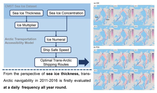
2. Materials and Methods

2.1. CMST Sea Ice Data

CMST spanning from 2011 to 2016 is a reanalysis sea ice dataset, generated by a regional, coupled ice–ocean model based on the Massachusetts Institute of Technology general circulation model (MITgcm) with sea ice data assimilation [25]. In detail, CryoSat-2 (CS2) SIT from Alfred Wegener Institute (AWI), Soil Moisture and Ocean Salinity (SMOS) SIT from University of Hamburg and Special Sensor Microwave Imager/Sounder (SSMIS) SIC from Integrated Climate Data Center are assimilated into the MITgcm ice–ocean model using a Local Error Subspace Transform Kalman filter coded in the Parallel Data Assimilation Framework (PDAF) [26]. The dynamics scheme used in MITgcm is the sea ice dynamics of a viscous plastic rheology [27,28], and the thermodynamics scheme is a one-layer, zero heat capacity formulation [29,30]. Driving MITgcm is the atmospheric ensemble forecasts from the United Kingdom Met Office (UKMO) Ensemble Prediction System [31]. CMST provides daily grid-cell-averaged SIT estimates all year round [23] and covers the smallest recorded ice extents in 2012 and 2016 [32,33]. The sea ice variables are discretized on an Arakawa C grid with a spatial resolution of 18 km. In previous validations, CMST reproduced most of the observed temporal and spatial variations of SIT compared with most available in situ observations in the Arctic Basin. CMST also shows some advantages over the statistically merged product, CS2 SMOS, and the Pan-Arctic Ice-Ocean Modeling and Assimilation System (PIOMAS) thickness product [23]. Low bias and errors between CMST and helicopter-borne electromagnetic induction sounding SIT and CS2 SIT are also found over the Fram Strait, suggesting a good performance of CMST SIT in this dynamical ice outflow region [34]. Overall, taking advantage of the all-year-round coverage and daily resolution in the temporal scale, the opening days, closing days and navigation windows of the Arctic shipping routes are first revisited in this study.

2.2. Methods of Navigability Estimation

SIC and SIT provided by CMST are used in a semiempirical Arctic Transportation Accessibility Model (ATAM) to assess navigability within the ice regime. Following Stephenson et al. [24], Ice Multipliers (IM) indicate the navigation risk in different sea ice conditions for the certain ice-resistance of vessels. In detail, IM for the two representative vessels investigated in this study, Open Water (OW) and Polar Class 6 (PC6) vessels, are given:
IM OW = { 2 ,   SIT = 0 1 ,   0   <   SIT   <   15 1 ,   15     SIT   <   70 2 ,   70     SIT   < 120   3 ,   120     SIT   <   151 4 ,   SIT     151 , IM PC 6 = { 2 ,   0     SIT   <   70 1 ,   70     SIT   <   120 1 ,   120     SIT   <   151 3 ,   151     SIT   <   189 4 ,   SIT     189
Then, the IM are operated with the Arctic Ice Regime Shipping System (AIRSS) [35] to assess the navigability for different kinds of vessels in the Arctic. In AIRSS, the ice numeral (IN) is given:
IN = ( C a   ×   IM a ) + ( C b   ×   IM b ) + + ( C n   ×   IM n )
where C a ,   C b , are the SIC in tenths of ice type a, b, , and IM a ,   IM b ,   are the Ice Multiplier (IM) for corresponding ice types. The IN is calculated for every grid cell of the dataset in every available day. A negative IN means the grid cell is unnavigable, while a positive or zero IN indicates the cell is navigable. A larger IN value equates to a smaller navigation risk.
Subsequently, a shortest path algorithm is applied to find OASR across the daily IN-gridded fields that costs minimal sailing time between the departure port and destination port [9,10]. Following McCallum [36], shipping transit time is derived from the grid cell range and the ship safe speed (SS) determined by the IN (Table 1). Therefore, the transit time is given as follows:
ST i = d i 1 / 2 SS i 1 + d i 2 / 2 SS i 2
where ST i is the transit time between the centers of grid cells i1 and i2, d i 1 and d i 2 are the distances between two cells’ centers and SS i 1 and SS i 2 are the ship safe speeds in these corresponding cells. Then, a weighted graph is obtained, whose node is the center point of each grid and the edge records the sailing time between nodes.
The Dijkstra algorithm [37] used here is a classic algorithm for finding the shortest paths between the starting nodes and target nodes in a weighed graph. It is applied to find the OASR between Atlantic ports (Rotterdam port or St. John’s port) and the Bering Strait ( 65 ° 38 36   N, 169 ° 11 42   W). Voyages along the Northern Sea Route (NSR) are determined as routes starting from the Rotterdam port ( 51 ° 55   N ,   4 ° 30   E ) and arriving at Bering Strait ( 65 ° 38 36   N, 169 ° 11 42   W). Additionally, voyages along the NWP begin from St. John’s port ( 47 ° 33 42   N ,   52 ° 37 54   W ) and end at the Bering Strait ( 65 ° 38 36   N, 169 ° 11 42   W).
Transit time and navigation windows can then be obtained from the daily OASR. A navigable day is defined as a day that the most time-saving route (i.e., OASR) can be found by the Dijkstra shortest path algorithm. The transit time between a starting port and the Bering Strait is subsequently integrated as the sailing time across an entire OASR. Following Liu et al. (2017), the start date of the navigation windows is defined as the first day of three consecutive, navigable days and the end date is defined as the first day of three consecutive, unnavigable days. All the navigation windows are searched from summer (June, July and August) to the winter (December, January and February) in each year because the opening and closing of the navigation windows occur over this period.

3. Results

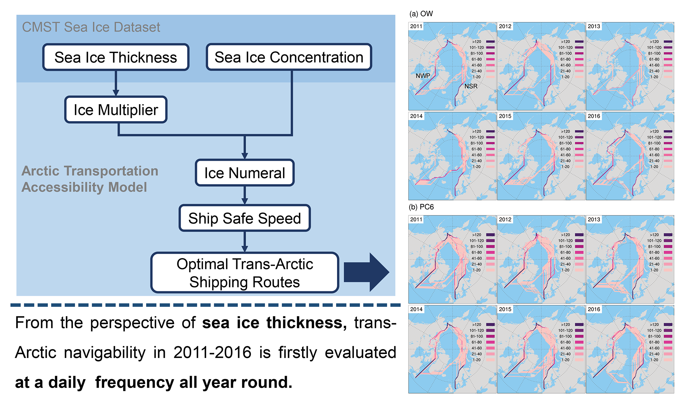
3.1. Optimal Trans-Arctic Shipping Routes (OASR)

The OASR from 2011 to 2016 (Figure 1a) show that OW vessels along the NSR in 2013 were rather limited and hindered by sea ice, with less than 60 independent routes identified. By contrast, with relatively lower sea ice cover along the NSR in 2011 and 2015, there was greater potential for OW vessels to sail along the NSR smoothly (i.e., more than 100 routes). Geographically, the OASRs of the NSR were further north than usual (especially in the segment of the Laptev Sea (LS) and the East Siberian Sea (ESS)) in 2012, corresponding with the lowest recorded ice extent in that summer [32].
Navigations along the NWP were also limited to less than 20 for OWs, and the northern subroute of NWP (i.e., the NWP via the M’Clure strait) was completely blocked in 2013 and 2014. The OASR map (Figure 1b) shows higher accessibility for PC6 vessels with a greater number of ideal routes and expanding geographic regions compared with OWs along both the NSR and NWP. Both the southern (i.e., the route of NWP except through the M’Clure strait) and northern subroutes of the NWP were passable for PC6 vessels from 2011 to 2016 owing to their stronger capacity for ice breaking. Moreover, there were more OASRs in the shorter northern subroute of the NWP in 2011 and 2012 compared with OW vessels.

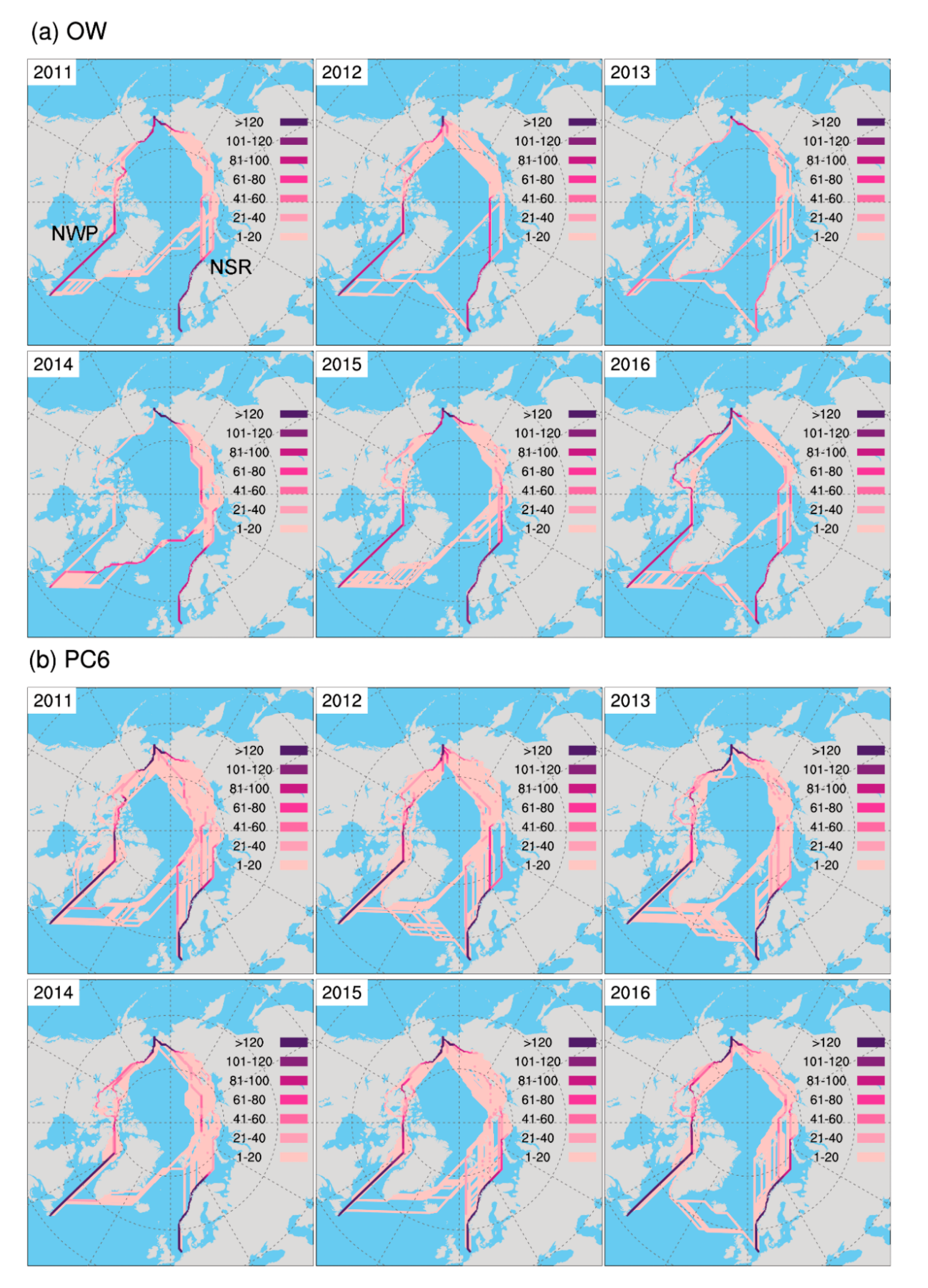
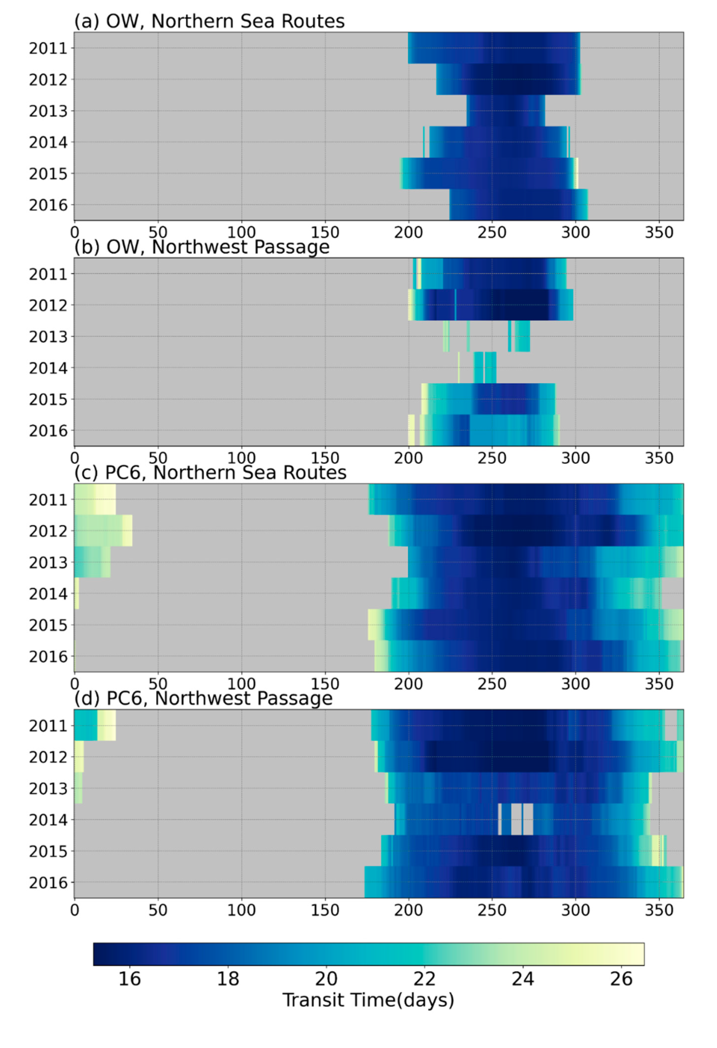
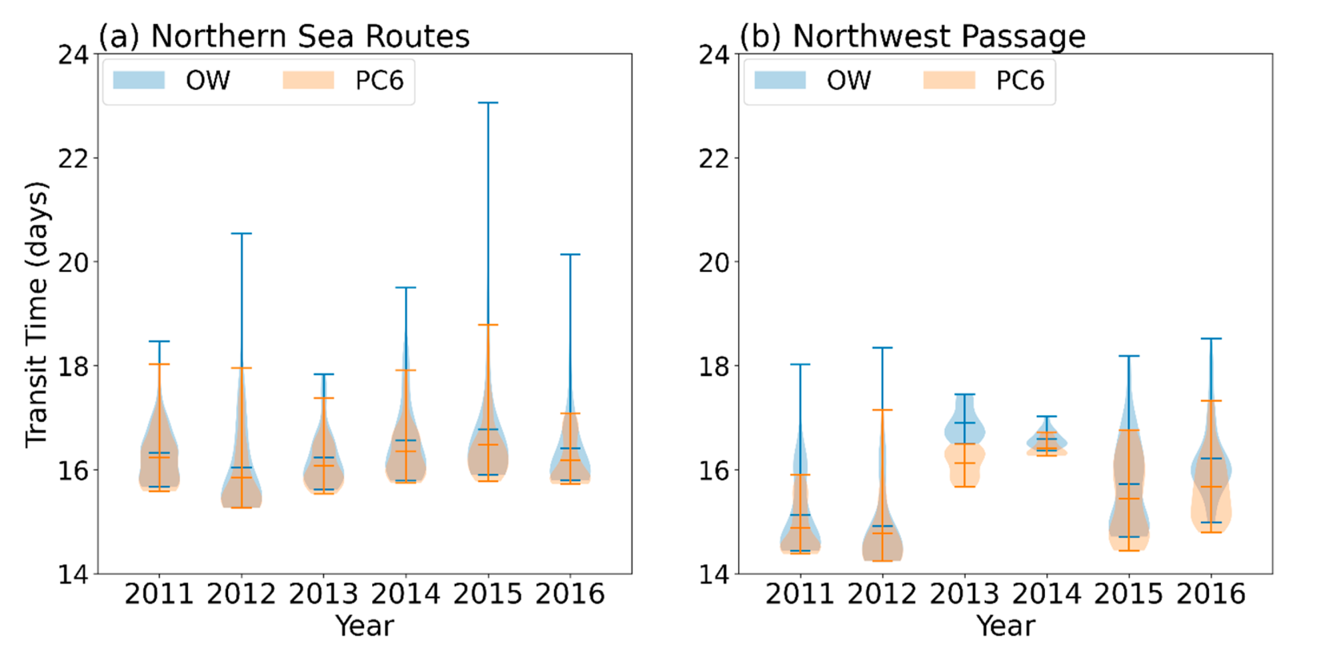
3.2. Daily Transit Time and Navigation Windows

Combining sea ice parameters from CMST and ATAM, daily transit times for OW and PC6 vessels via the NSR and the NWP are compared with each other (Figure 2). On average, the transit time for OW and PC6 vessels sailing along the NSR dropped to around 16–17 days after the start date of navigation window and then raised when the freezing season (October–April) was coming (Figure 2a,c); however, for the NWP, OW vessels had large uncertainty on the transit time and the passage was almost completely hindered in 2013 and 2014.
In general, PC6 vessels underwent less ice-blockage than OW vessels, especially when sailing in the NWP, and had longer navigation windows in both the NSR and the NWP. Fewer interruptions of the consecutive navigable days occurred in the middle/latter navigation windows in the NWP in 2014/2011.
Statistical information on transit time including the minimum, maximum and mean values is given by a ‘violin plot’ (Figure 3). Additionally, the frequency distribution of transit time is shown by the width of each violin. The minimum transit time for OW vessels in the NSR was about 15 days in 2012, while the mean was 16–17 days (Figure 3a); thus, the distribution of transit time was highly skewed. The maximum transit time of each year showed larger variability for OWs sailing along the NSR; it was only about 18 days in 2013 but reached 23 days in 2015. This large fluctuation was related to the length of the navigation windows. At the beginning and end of the navigation window, the ship generally had a slower speed and spent longer transit time than over the mid-period of the navigation window (Figure 2). For this reason, although the navigation window in 2015 was longer than in 2013, the maximum transit time in 2015 was larger than that in 2013. Focusing on the navigation conditions of PC6 vessels, the yearly minimum transit time was very close to that of OW vessels because the NSR had nearly opened and the ship safe speeds in open water were the same for the OW and PC6 vessels. The maximum transit time of PC6 vessels was less than OW vessels. For instance, it took about 19 days for PC6s but 23 days for OWs along the NSR in 2015.
Sailing along the NWP costed a minimum of 14–15 days and a mean of 15–16 days for OW vessels, except in 2013 and 2014. Transit time in 2013 and 2014 was longer than in other years, with the mean transit time of about 17 days and a minimum of 16 days. The slower navigation can be attributed to the slowing of ship safe speed by thicker ice (Table 1), especially in the northern subroute of the NWP. For PC6 vessels, the maximum and mean transit times were much shorter than those of OW vessels within the overlapping navigation windows because of their stronger ice-breaking capability and relatively high sailing speed.
The navigation windows are quantified in this study; additionally, the mean and standard deviation of navigation windows are calculated from the total navigable days of each year (Table 2 and Table 3). Sailing along the NSR had successive navigation windows for both OW and PC6 vessels each year. For the NWP, however, the interruption of the consecutive navigable days occurred more frequently and, thus, resulted in several discontinuous navigation windows for both OW and PC6 vessels (Table 4 and Table 5). The shortest navigation window of 47 days for OW vessels along the NSR happened in 2013, which was 45% shorter than the mean navigation window (85 ± 21 days) of 2011–2016. The early closing in October was due to the thicker ice remaining in the Arctic in summer 2013 together with an earlier freeze onset in that cold year [38]. We also find the range in the start date was much larger than the range in the end date for OW vessels, i.e., 5–6 weeks versus 3–4 weeks. The mean navigation window and its standard deviation for PC6 vessels were about 189 ± 25 days along the NSR. However, due to the blockage of thick ice in the ESS, PC6 vessels had relatively shorter navigation windows in 2013 and 2014. The length of navigation windows reached its minimum (162 days) in 2014 and was 13% shorter than the average from 2011–2015. Therefore, both OW and PC6 vessels reached their minimum navigation windows in 2013 and 2014, respectively.
As shown in Table 4 and Table 5, OW vessels had a mean navigation window of 64 days with significant variability of 40 days standard deviation along the NWP. The main reason for this large standard deviation was because the NWP was almost unnavigable all year for OW vessels in both 2013 and 2014. Nevertheless, PC6 vessels along the NWP had a mean navigation window of 169 days and a smaller standard deviation of 20 days compared to that of the NSR. Due to the obstruction from sea ice in CAA, two separate navigation windows of about 70 days were found for PC6 vessels along the NWP in 2014. In contrast, with less sea ice obstruction in the CAA [39], the relatively longer navigation windows of the NWP for both OW and PC6 vessels occurred in 2011 and 2012. Moreover, whether sailing along the NSR or NWP, the navigable days for PC6 vessels were conspicuously more numerous than those for OW vessels.

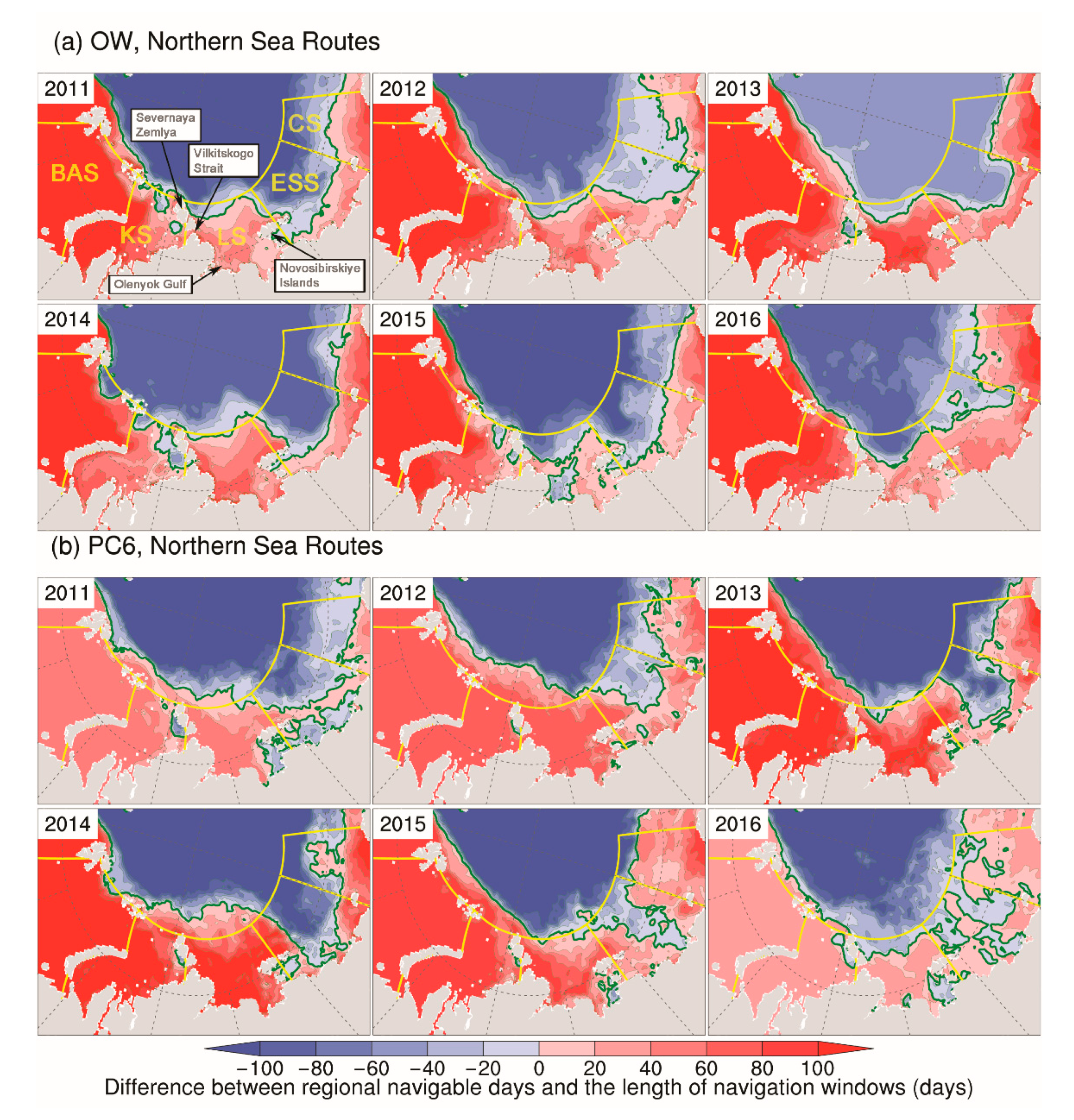
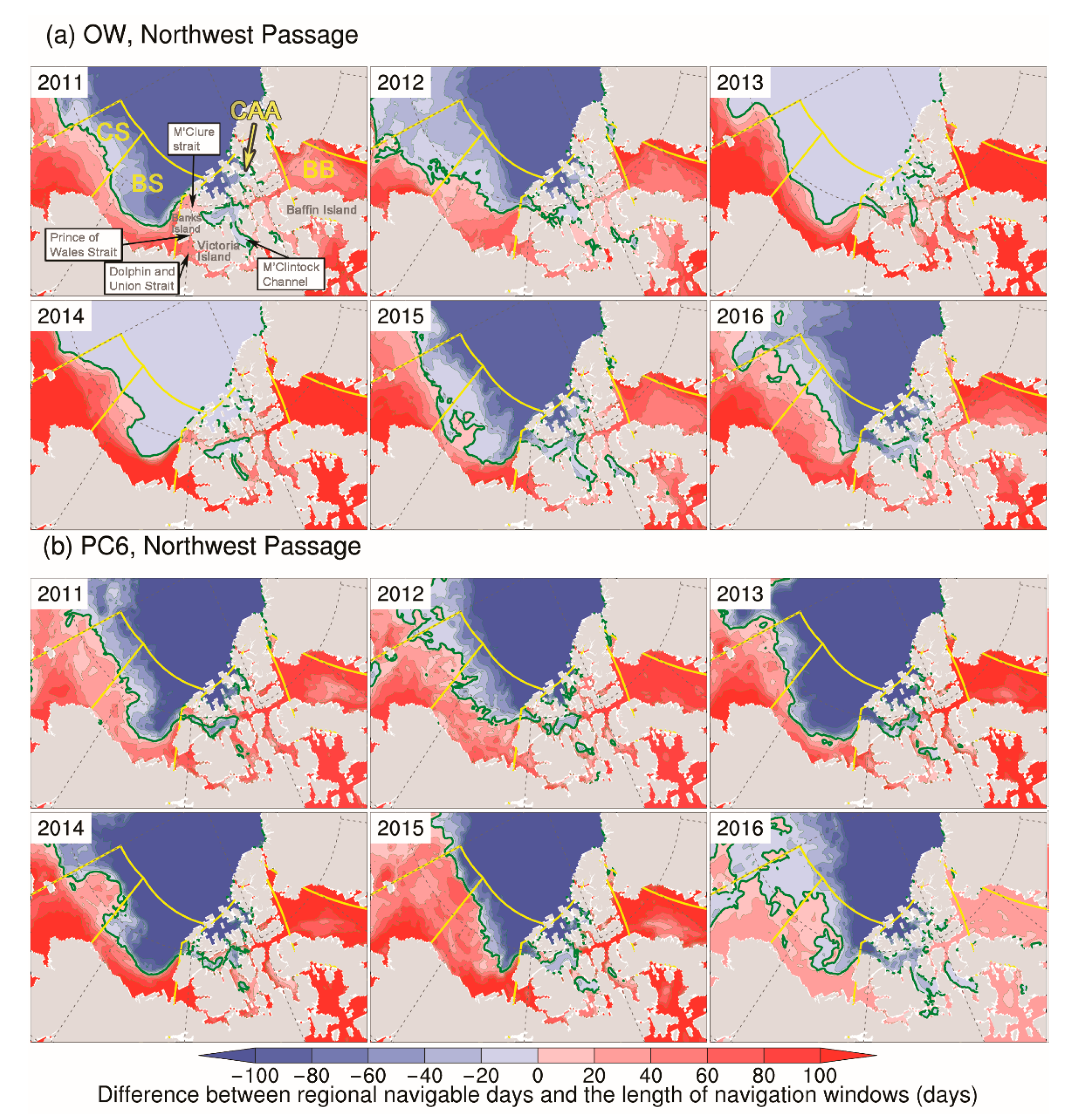
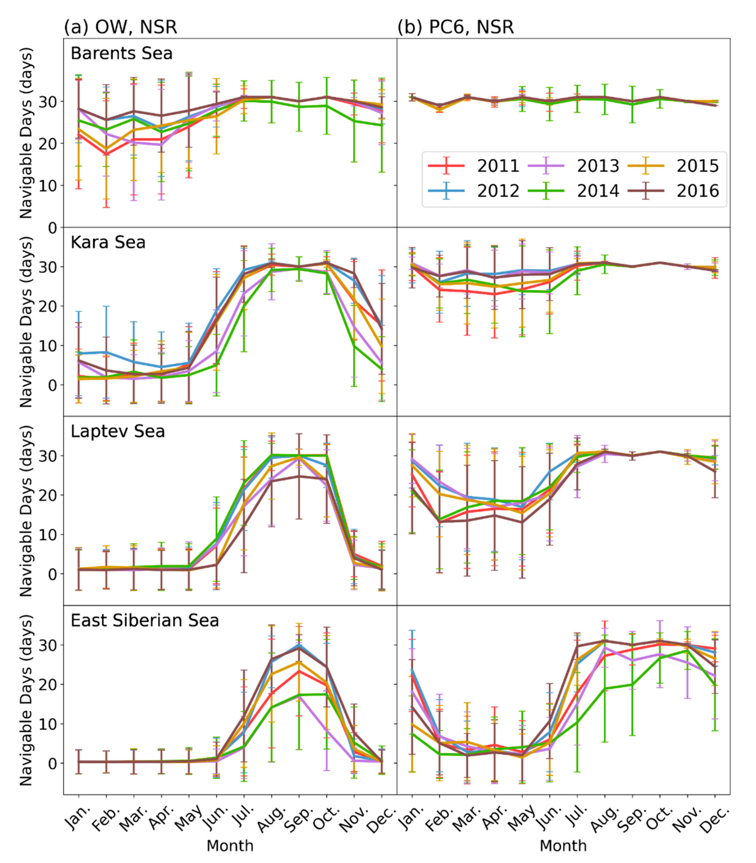
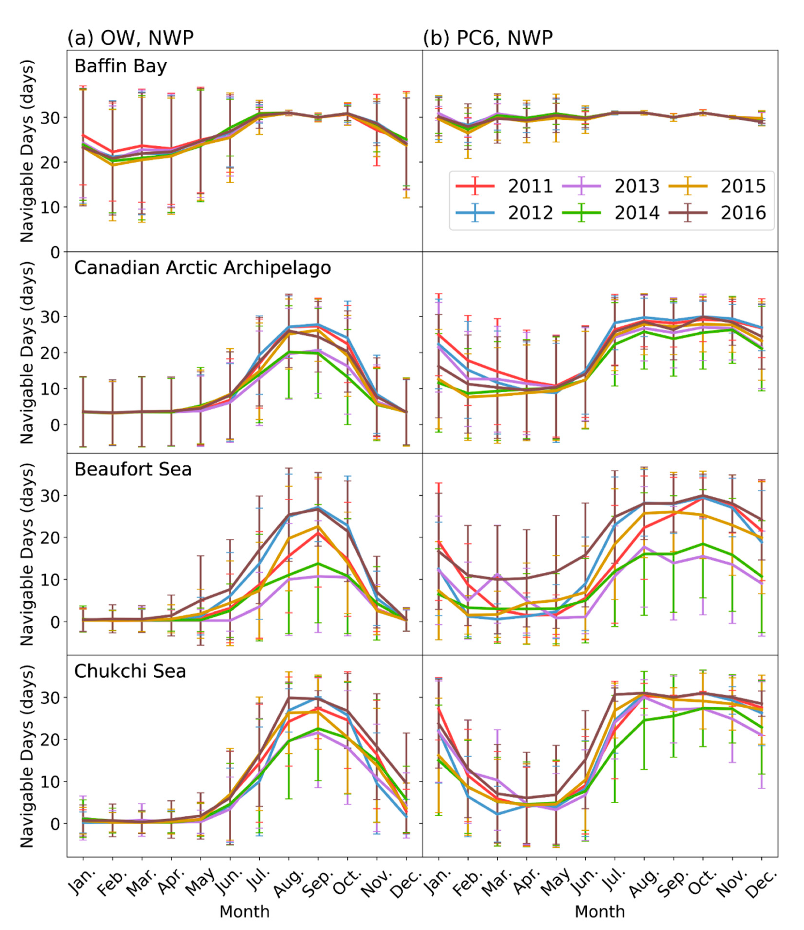
3.3. Regional Navigability

Local variations of navigable periods in different subseas of a route can influence the length of entire trans-Arctic navigation windows. To show the detailed spatiotemporal navigational variations along the NSR and NWP, the difference between the accumulated navigable days (i.e., number of days that IN > 0 in a certain grid cell) and the length of the navigation windows for OW and PC6 vessels are drawn in Figure 4 and Figure 5 annually. A negative anomaly (difference ≤ 0) represents where the navigable days in such a region is less than the navigation windows, indicating that regions limit the opening of trans-Arctic passages. Inversely, the areas with a positive anomaly (difference > 0) have little impact on the navigation windows—this can be interpreted as ‘barrel effect’. As extensive areas with positive anomaly were found, most parts of the Barents Sea (BAS) were navigable all year for both OW and PC6 vessels. The Kara Sea (KS) and Laptev Sea (LS) also had wide areas of positive anomaly compared to the navigation window for both OW and PC6 vessels, except areas near the Severnaya Zemlya and Vilkitskogo Strait, especially for OW vessels. There were large areas with negative anomaly in the LS (e.g., Olenyok Gulf) in 2015, which might shorten the navigation windows of NSR in that year. The East Siberian Sea (ESS) was another key region that had a significant impact on the whole NSR because of its locally few navigable days and significant interannual variability. For example, in 2015, the navigation conditions in the ESS were greatly limited and thus shortened the navigation window of the NSR by interrupting the continuity of the entire OASR. The areas around the Novosibirskiye Islands had similar navigable days with the ESS. Albeit large areas of negative anomaly were found in Chukchi Sea (CS) for OW and PC6 vessels, the south part of this sea was still with positive anomaly for finding the entire OASR. In general, the Vilkitskogo Strait and also the ESS were vital for the navigations via the NSR because the areas with negative anomaly usually occurred in these regions.
As shown in Figure 5, there was a positive anomaly in most regions of the Baffin Bay (BB) for both OW and PC6 vessels in all years. The areas close to the Baffin Island were not perennially accessible because the thick ice (>1.2 m) was located east of Baffin Island in March [40]. The navigable days in the CAA were almost with negative anomaly for both vessels because thick ice obstructed the narrow strait, especially in the northwest of the CAA. The northern part of the Beaufort Sea (BS) also had shorter navigable days for OW and PC6 vessels. As for the CS, it showed much longer navigable days compared with the navigation window of the NWP. In general, the most obvious negative anomaly occurred in the BS and CAA, implying that they were the key regions for enabling or disabling ship access along the NWP.
To reveal the seasonal and interannual variation of navigable days in different seas, we calculated the regional-average navigable days along the NSR and NWP (shown in Figure 6 and Figure 7). The seasonal variation of navigable days in the BAS was limited, especially for PC6 vessels. The shortest navigable days (at least about 20) for OW vessels in the BAS were found during the first half of the year; however, more distinct seasonality and interannual variation of locally navigable days were found in the KS and LS. The size of the error bars and differences between years were largest in ESS for both OW and PC6 vessels, particularly in the summer months. In detail, the maximum navigable days were usually in August, September and October for OW vessels. The NSR was almost unnavigable in all areas from February to May. For PC6 vessels, there were about 30 navigable days, with small standard deviations in the KS and LS from July to December. Again, the largest interannual variation occurred in the ESS, indicating that the ESS was a key subregion for shipping along the NSR. For example, the monthly averaged navigable days for OW vessels were limited to about 17 days in September in 2013 and 2014, while that can reach 30 days in 2012 and 2016. Overall, the sea ice conditions in the BAS had little impact on the navigation of OW and PC6 vessels, as did KS for PC6 vessels.
Similarly, both seasonal and interannual cycles can also be found in the NWP (Figure 7). The BB was the only region that always had more than 20 navigable days for both OW and PC6 vessels but with unobvious seasonality, especially for PC6 vessels. Distinct seasonality occurred in the CAA, BS and CS, and large interannual cycles were found in the BS and CS. Especially, in the BS, the mean navigable days for OW vessels in September were only 9 days in 2013 and 11 days in 2014, followed by about 23 days in 2015. However, in 2016, PC6 vessels had distinctly more navigable days in the BS. We thus inferred that BS is a key subregion for shipping along the NWP owing to its largest difference between years and standard deviation. The interannual cycle of navigable days in the CAA and CS were similar to the BS but the interannual disparities were small.

4. Discussion and Conclusions

This study aimed to assess the OASR with ATAM and CMST sea ice analysis on a daily frequency for the first time. Then, navigation window and transit time at daily frequency were estimated. These assessments have great significance on Arctic shipping and will offer a practical reference for shipping companies and stakeholders. Intense interannual variability of navigability was found in 2011–2016 due to the extreme cases of sea ice conditions in different years. The seaworthiness along the NSR and NWP for both OW and PC6 vessels was poor in 2013 and 2014, with shorter navigation windows and longer transit time. OW vessels along the NSR had longer navigation windows in 2011 and 2015, while the OASR that cost the least transit time expanded further northward in 2012. As for the NWP, the navigation windows for OW and PC6 vessels were longer, with more subnorthern routes opening in 2011 and 2012. This different navigability between the NSR and the NWP was mainly associated with the varied MYI in the NWP [41,42,43,44,45]. The analysis of regional navigability (Figure 6 and Figure 7) revealed the interannual variability and seasonality for shipping along the NSR and NWP. The areas near Vilkitskogo Strait (especially parts within the LS), Novosibirskiye Islands and ESS in the NSR, as well as the CAA and BS in the NWP had much shorter navigable days than the other regions. Thus, these keystone regions had disproportionate impacts on the navigability of the entire NSR and NWP and their navigation windows.
Benefiting from the daily resolution of the CMST dataset, the estimation of navigation windows could be closely connected with actual shipping activities rather than relying on monthly mean SIT. The estimates of navigation windows revealed that there were some interruptions between navigable days of the NWP (Figure 2), resulting in discontinuous navigation windows in some years (i.e., for OW vessels in 2013 and 2016 and for PC6 vessels in 2011 and 2014). These gaps in navigation windows were the result of occlusions in the CAA occurring in varied locations in different years. For instance, the M’Clintock Channel located to the west of the Prince of Wales Island was blocked in 2014; the Prince of Wales Strait and the Dolphin and Union Strait located in the west of the Victoria Island were occluded in 2011. For more accurate estimation of navigability, especially in these key straits and seas, higher spatial and temporal resolution in sea ice monitoring are required in future studies [13]. Meanwhile, the ability to simulate heavily deformed and ridged sea ice in the MYI regions (e.g., the CAA) still needs improvements in numerical simulations and forecasts [23]. Limited by the period of CMST sea ice data, the time period assessed in this study is only 6 years, which is too short.
Assessment of Arctic navigability in this study only focuses on sea ice conditions; however, beyond that, the operation of Arctic shipping routes is also affected by elements such as wind, fog and ocean waves [46,47,48]. Bathymetry constraint is another factor that is particularly significant for large vessels with big breadth and deep draft that use Arctic shipping routes in shallower waters. In addition, maritime technology, commercial profit (e.g., ice-breaking services and infrastructure investment) and political jurisdiction are significant concerns [47,49,50]. These hazards for shipping are not considered in this work and should be explored in short-term forecasts for actual navigation. We also acknowledge that the time span of CMST is short at six years and, thus, cannot identify climate-induced trends in Arctic shipping navigability. A long-term study of OASR at a daily frequency is crucial for stakeholders under the background of decadal climate-induced sea ice decline.

Author Contributions

Q.Y. and C.M. conceptualized this study; X.Z. and C.M. carried out this study, performed the calculations and drafted the paper; Y.Y., J.C.L., L.M. and Q.Y. processed the review and editing of the paper. All authors have read and agreed to the published version of the manuscript.

Funding

This study was funded by Southern Marine Science and Engineering Guangdong Laboratory (Zhuhai) (NO. SML2020sp007), National Natural Science Foundation of China (No. 41922044, 41941009, 41676185), the Guangdong Basic and Applied Basic Research Foundation (No. 2020B1515020025), and CAS “Light of West China” Program (E129030101, Y929641001). J.L. acknowledges support from the Centre for Integrated Remote Sensing and Forecasting for Arctic Operations (CIRFA) project through the Research Council of Norway (RCN) under Grant #237906.

Institutional Review Board Statement

Not applicable.

Informed Consent Statement

Not applicable.

Data Availability Statement

The CMST sea-ice thickness and drift data can be downloaded from https://doi.org/10.1594/PANGAEA.891475 (Mu et al., 2018b; accessed on 27 February 2020).

Acknowledgments

This is a contribution to the Year of Polar Prediction (YOPP), a flagship activity of the Polar Prediction Project (PPP), initiated by the World Weather Research Programme (WWRP) of the World Meteorological Organization (WMO). We would like to thank Hajo Eicken at the International Arctic Research Center, University of Alaska Fairbanks for his constructive advice to improve this study.

Conflicts of Interest

The authors declare no conflict of interest.

References

  1. Solomon, S.; Manning, M.; Marquis, M.; Qin, D. Climate Change 2007-the Physical Science Basis: Working Group I Contribution to the Fourth Assessment Report of the IPCC; Cambridge University Press: Cambridge, UK, 2007; Volume 4. [Google Scholar]
  2. Serreze, M.C.; Francis, J.A. The Arctic amplification debate. Clim. Chang. 2006, 76, 241–264. [Google Scholar] [CrossRef] [Green Version]
  3. Screen, J.A.; Simmonds, I. The central role of diminishing sea ice in recent Arctic temperature amplification. Nature 2010, 464, 1334–1337. [Google Scholar] [CrossRef] [PubMed] [Green Version]
  4. Kwok, R. Arctic sea ice thickness, volume, and multiyear ice coverage: Losses and coupled variability (1958–2018). Environ. Res. Lett. 2018, 13, 105005. [Google Scholar] [CrossRef]
  5. Comiso, J.C.; Parkinson, C.L.; Gersten, R.; Stock, L. Accelerated decline in the Arctic sea ice cover. Geophys. Res. Lett. 2008, 35. [Google Scholar] [CrossRef] [Green Version]
  6. Holland, M.M.; Bitz, C.M.; Tremblay, B. Future abrupt reductions in the summer Arctic sea ice. Geophys. Res. Lett. 2006, 33. [Google Scholar] [CrossRef] [Green Version]
  7. Wang, M.; Overland, J.E. A sea ice free summer Arctic within 30 years: An update from CMIP5 models. Geophys. Res. Lett. 2012, 39. [Google Scholar] [CrossRef] [Green Version]
  8. Onarheim, I.H.; Eldevik, T.; Smedsrud, L.H.; Stroeve, J.C. Seasonal and regional manifestation of Arctic sea ice loss. J. Clim. 2018, 31, 4917–4932. [Google Scholar] [CrossRef]
  9. Smith, L.C.; Stephenson, S.R. New Trans-Arctic shipping routes navigable by midcentury. Proc. Natl. Acad. Sci. USA 2013, 110, E1191–E1195. [Google Scholar] [CrossRef] [Green Version]
  10. Melia, N.; Haines, K.; Hawkins, E. Sea ice decline and 21st century trans-Arctic shipping routes. Geophys. Res. Lett. 2016, 43, 9720–9728. [Google Scholar] [CrossRef]
  11. Khon, V.C.; Mokhov, I.I.; Semenov, V.A. Transit navigation through Northern Sea Route from satellite data and CMIP5 simulations. Environ. Res. Lett. 2017, 12, 024010. [Google Scholar] [CrossRef] [Green Version]
  12. Schøyen, H.; Bråthen, S. The Northern Sea Route versus the Suez Canal: Cases from bulk shipping. J. Transp. Geogr. 2011, 19, 977–983. [Google Scholar] [CrossRef]
  13. Mäkynen, M.; Haapala, J.; Aulicino, G.; Balan-Sarojini, B.; Balmaseda, M.; Gegiuc, A.; Girard-Ardhuin, F.; Hendricks, S.; Heygster, G.; Istomina, L. Satellite observations for detecting and forecasting sea-ice conditions: A summary of advances made in the SPICES project by the EU’s Horizon 2020 programme. Remote Sens. 2020, 12, 1214. [Google Scholar] [CrossRef] [Green Version]
  14. Stephenson, S.R.; Brigham, L.W.; Smith, L.C. Marine accessibility along Russia's Northern Sea Route. Polar Geogr. 2013, 37, 111–133. [Google Scholar] [CrossRef]
  15. Khon, V.C.; Mokhov, I.I.; Latif, M.; Semenov, V.A.; Park, W. Perspectives of Northern Sea Route and Northwest Passage in the twenty-first century. Clim. Chang. 2009, 100, 757–768. [Google Scholar] [CrossRef]
  16. Stephenson, S.R.; Smith, L.C.; Brigham, L.W.; Agnew, J.A. Projected 21st-century changes to Arctic marine access. Clim. Chang. 2013, 118, 885–899. [Google Scholar] [CrossRef] [Green Version]
  17. Mokhov, I.I.; Khon, V.C.; Prokof’eva, M.A. New model estimates of changes in the duration of the navigation period for the Northern Sea Route in the 21st century. Dokl. Earth Sci. 2016, 468, 641–645. [Google Scholar] [CrossRef]
  18. Wei, T.; Yan, Q.; Qi, W.; Ding, M.; Wang, C. Projections of Arctic sea ice conditions and shipping routes in the twenty-first century using CMIP6 forcing scenarios. Environ. Res. Lett. 2020, 15, 104079. [Google Scholar] [CrossRef]
  19. Stephenson, S.R.; Smith, L.C. Influence of climate model variability on projected Arctic shipping futures. Earths Future 2015, 3, 331–343. [Google Scholar] [CrossRef] [Green Version]
  20. Melia, N.; Haines, K.; Hawkins, E.; Day, J.J. Towards seasonal Arctic shipping route predictions. Environ. Res. Lett. 2017, 12, 084005. [Google Scholar] [CrossRef]
  21. Stern, D.P.; Doyle, J.D.; Barton, N.P.; Finocchio, P.M.; Komaromi, W.A.; Metzger, E.J. The Impact of an Intense Cyclone on Short-Term Sea Ice Loss in a Fully Coupled Atmosphere-Ocean-Ice Model. Geophys. Res. Lett. 2020, 47, e2019GL085580. [Google Scholar] [CrossRef]
  22. Caballero, R.; Woods, C. The Role of Moist Intrusions in Winter Arctic Warming and Sea Ice Decline. J. Clim. 2016, 29, 4473–4485. [Google Scholar] [CrossRef]
  23. Mu, L.; Losch, M.; Yang, Q.; Ricker, R.; Losa, S.N.; Nerger, L. Arctic-Wide Sea Ice Thickness Estimates From Combining Satellite Remote Sensing Data and a Dynamic Ice-Ocean Model with Data Assimilation During the CryoSat-2 Period. J. Geophys. Res. Ocean. 2018, 123, 7763–7780. [Google Scholar] [CrossRef] [Green Version]
  24. Stephenson, S.R.; Smith, L.C.; Agnew, J.A. Divergent long-term trajectories of human access to the Arctic. Nat. Clim. Chang. 2011, 1, 156–160. [Google Scholar] [CrossRef]
  25. Marshall, J.; Adcroft, A.; Hill, C.; Perelman, L.; Heisey, C. A finite-volume, incompressible Navier Stokes model for studies of the ocean on parallel computers. J. Geophys. Res. Ocean. 1997, 102, 5753–5766. [Google Scholar] [CrossRef] [Green Version]
  26. Nerger, L.; Hiller, W. Software for ensemble-based data assimilation Systems—Implementation strategies and scalability. Comput. Geosci. 2013, 55, 110–118. [Google Scholar] [CrossRef] [Green Version]
  27. Zhang, J.; Hibler, W., III. On an efficient numerical method for modeling sea ice dynamics. J. Geophys. Res. Ocean. 1997, 102, 8691–8702. [Google Scholar] [CrossRef]
  28. Hibler, W., III. A dynamic thermodynamic sea ice model. J. Phys. Oceanogr. 1979, 9, 815–846. [Google Scholar] [CrossRef] [Green Version]
  29. Parkinson, C.L.; Washington, W.M. A large-scale numerical model of sea ice. J. Geophys. Res. Ocean. 1979, 84, 311–337. [Google Scholar] [CrossRef]
  30. Semtner, A.J., Jr. A model for the thermodynamic growth of sea ice in numerical investigations of climate. J. Phys. Oceanogr. 1976, 6, 379–389. [Google Scholar] [CrossRef] [Green Version]
  31. Bougeault, P.; Toth, Z.; Bishop, C.; Brown, B.; Burridge, D.; Chen, D.H.; Ebert, B.; Fuentes, M.; Hamill, T.M.; Mylne, K. The THORPEX interactive grand global ensemble. Bull. Am. Meteorol. Soc. 2010, 91, 1059–1072. [Google Scholar] [CrossRef]
  32. Parkinson, C.L.; Comiso, J.C. On the 2012 record low Arctic sea ice cover: Combined impact of preconditioning and an August storm. Geophys. Res. Lett. 2013, 40, 1356–1361. [Google Scholar] [CrossRef]
  33. Petty, A.A.; Stroeve, J.C.; Holland, P.R.; Boisvert, L.N.; Bliss, A.C.; Kimura, N.; Meier, W.N. The Arctic sea ice cover of 2016: A year of record-low highs and higher-than-expected lows. Cryosphere 2018, 12, 433–452. [Google Scholar] [CrossRef] [Green Version]
  34. Min, C.; Mu, L.; Yang, Q.; Ricker, R.; Shi, Q.; Han, B.; Wu, R.; Liu, J. Sea ice export through the Fram Strait derived from a combined model and satellite data set. Cryosphere 2019, 13, 3209–3224. [Google Scholar] [CrossRef] [Green Version]
  35. Transport Canada. Arctic Ice Regime Shipping System (AIRSS) Standards; Transport Canada: Ottawa, ON, Canada, 1998. [Google Scholar]
  36. McCallum, J. Safe Speed in Ice: An Analysis of Transit Speed and Ice Decision Numerals; Ship Safety Northern (AMNS), Transport Canada: Ottawa, ON, Canada, 1996. [Google Scholar]
  37. Dijkstra, E.W. A note on two problems in connexion with graphs. Numer. Math. 1959, 1, 269–271. [Google Scholar] [CrossRef] [Green Version]
  38. Tilling, R.L.; Ridout, A.; Shepherd, A.; Wingham, D.J. Increased Arctic sea ice volume after anomalously low melting in 2013. Nat. Geosci. 2015, 8, 643–646. [Google Scholar] [CrossRef] [Green Version]
  39. Howell, S.; Wohlleben, T.; Komarov, A.; Pizzolato, L.; Derksen, C. Recent extreme light sea ice years in the Canadian Arctic Archipelago: 2011 and 2012 eclipse 1998 and 2007. Cryosphere 2013, 7, 1753–1768. [Google Scholar] [CrossRef] [Green Version]
  40. Min, C.; Yang, Q.; Mu, L.; Kauker, F.; Ricker, R. Ensemble-based estimation of sea-ice volume variations in the Baffin Bay. Cryosphere 2021, 15, 169–181. [Google Scholar] [CrossRef]
  41. Howell, S.E.; Duguay, C.R.; Markus, T. Sea ice conditions and melt season duration variability within the Canadian Arctic Archipelago: 1979–2008. Geophys. Res. Lett. 2009, 36. [Google Scholar] [CrossRef]
  42. Kwok, R. Sea ice convergence along the Arctic coasts of Greenland and the Canadian Arctic Archipelago: Variability and extremes (1992–2014). Geophys. Res. Lett. 2015, 42, 7598–7605. [Google Scholar] [CrossRef]
  43. Mudryk, L.R.; Derksen, C.; Howell, S.; Laliberté, F.; Thackeray, C.; Sospedra-Alfonso, R.; Vionnet, V.; Kushner, P.J.; Brown, R. Canadian snow and sea ice: Historical trends and projections. Cryosphere 2018, 12, 1157–1176. [Google Scholar] [CrossRef] [Green Version]
  44. Dauginis, A.L.; Brown, L.C. Sea ice and snow phenology in the Canadian Arctic Archipelago from 1997 to 2018. Arct. Sci. 2020, 7, 1–26. [Google Scholar]
  45. Pizzolato, L.; Howell, S.E.L.; Dawson, J.; Laliberté, F.; Copland, L. The influence of declining sea ice on shipping activity in the Canadian Arctic. Geophys. Res. Lett. 2016, 43, 12–146. [Google Scholar] [CrossRef]
  46. Aksenov, Y.; Popova, E.E.; Yool, A.; Nurser, A.J.G.; Williams, T.D.; Bertino, L.; Bergh, J. On the future navigability of Arctic sea routes: High-resolution projections of the Arctic Ocean and sea ice. Mar. Policy 2017, 75, 300–317. [Google Scholar] [CrossRef] [Green Version]
  47. Buixadé Farré, A.; Stephenson, S.R.; Chen, L.; Czub, M.; Dai, Y.; Demchev, D.; Efimov, Y.; Graczyk, P.; Grythe, H.; Keil, K. Commercial Arctic shipping through the Northeast Passage: Routes, resources, governance, technology, and infrastructure. Polar Geogr. 2014, 37, 298–324. [Google Scholar] [CrossRef]
  48. Hill, E.; LaNore, M.; Véronneau, S. Northern sea route: An overview of transportation risks, safety, and security. J. Transp. Secur. 2015, 8, 69–78. [Google Scholar] [CrossRef]
  49. Lasserre, F. Case studies of shipping along Arctic routes. Analysis and profitability perspectives for the container sector. Transp. Res. Part A Policy Pract. 2014, 66, 144–161. [Google Scholar] [CrossRef]
  50. Milaković, A.-S.; Gunnarsson, B.; Balmasov, S.; Hong, S.; Kim, K.; Schütz, P.; Ehlers, S. Current status and future operational models for transit shipping along the Northern Sea Route. Mar. Policy 2018, 94, 53–60. [Google Scholar] [CrossRef]
Figure 1. ATAM-derived optimal trans-Arctic shipping routes (OASR) for (a) OW vessels and (b) PC6 vessels from 2011 to 2016. All the routes start from the Atlantic ports and end in the Pacific Bering Strait across the Arctic. Line colors indicate the number of optimal routes at the same location.
Remotesensing 13 02766 g001
Figure 2. Annual distribution of daily shortest transit time for OW and PC6 vessels (a,c) via the NSR and (b,d) via the NWP. The fill color indicates the trans-Arctic time through specific routes on certain days of the year, where the gray parts represent the unnavigable period and a day with filled color represents a navigable day.
Remotesensing 13 02766 g002
Figure 3. Violin plot of transit time for (a) the NSR and (b) the NWP. Transit time for OW is shown in light blue ‘violin plot’ and the light orange ‘violin plot’ denotes the transit time for PC6 vessels. The width of ‘violin plot’ represents the frequency distribution of transit time for the NSR and NWP. The short lines from top to bottom represent the maximum, mean and minimum values of the transit time.
Remotesensing 13 02766 g003
Figure 4. Regional anomaly of navigable days along the NSR for (a) OW vessels and (b) PC6 vessels. The fill color represents difference between the navigable days in a certain grid cell and the length of the annual navigation windows from 2011 to 2016. Green lines are the zero-lines of the anomaly. Yellow lines are the sea borders from the Multisensor Analyzed Sea Ice Extent (MASIE) Arctic Regions developed by the NSIDC (https://nsidc.org/data/masie/browse_regions, accessed on 20 March 2020). The seas from left to right are the Barents Sea (BAS), Kara Sea (KS), Laptev Sea (LS), East Siberian Sea (ESS) and Chukchi Sea (CS).
Remotesensing 13 02766 g004
Figure 5. The same as Figure 4, but for (a) OW vessels and (b) PC6 vessels along the NWP. The seas from left to right are the Chukchi Sea (CS), Beaufort Sea (BS), Canadian Arctic Archipelago (CAA) and Baffin Bay (BB).
Remotesensing 13 02766 g005
Figure 6. Regional navigable days along the NSR in 2011–2016. Color lines represent the time series of the monthly and regional-average navigable days for (a) OW vessels and (b) PC6 vessels within the BAS, KS, LS and ESS. Error bars are the standard deviation for regional grids.
Remotesensing 13 02766 g006
Figure 7. The same as Figure 6, but for (a) OW vessels and (b) PC6 vessels along the NWP. The time series from top to bottom are for the BB, CAA, BS and CS.
Remotesensing 13 02766 g007
Table 1. Ship safe speed (SS) in nautical miles per hour (nm/h) by Ice Numeral (IN) [9,24,36].
Ice NumeralShip Safe Speed (nm/h)
<00 (unnavigable or unsafe)
0–84
9–135
14–156
167
178
189
1910
2011
Table 2. Navigation start date, end date and length of navigation windows for OW vessels along the NSR in 2011–2016.
NSR/OWNavigation
Start Date
Navigation
End Date
Navigation
Window Length
201107–2010–31103
201208–0510–3187
201308–2410–1047
201408–0210–2584
201507–1510–30107
201608–1311–0483
Mean and standard deviation of navigation windows85 ± 21
Table 3. Navigation start date, end date and length of navigation windows for PC6 vessels along the NSR in 2011–2016. Note that the closing date in 2016 can be detected in the next year.
NSR/PC6Navigation Start DateNavigation End DateNavigation
Window Length
201106–2602–05224
201207–0701–22199
201307–2001–04168
201407–1012–19162
201506–2601–02190
201606–29//
Mean and standard deviation of navigation windows189 ± 25
Table 4. The same as Table 2, but for the NWP.
NWP/OWNavigation Start DateNavigation End DateNavigation Window Length
201126 July23 October89
201219 July26 October99
201310 August14 August4
22 September1 October9
201428 August11 September14
201528 July17 October81
201619 July23 July4
26 July18 October84
Mean and standard deviation of navigation windows64 ± 40
Table 5. The same as Table 3, but for the NWP.
NWP/PC6Navigation Start DateNavigation End DateNavigation Window Length
201128 June21 December176
28 December7 January10
201229 June5 January190
20136 July13 December160
201412 July20 September70
3 October12 December70
20154 July22 December171
201623 June//
Mean and standard deviation of navigation windows169 ± 20
Publisher’s Note: MDPI stays neutral with regard to jurisdictional claims in published maps and institutional affiliations.

