Article

Evaluation of 2-m Air Temperature and Surface Temperature from ERA5 and ERA-I Using Buoy Observations in the Arctic during 2010–2020

1
School of Geospatial Engineering and Science, Sun Yat-Sen University, and Southern Marine Science and Engineering Guangdong Laboratory (Zhuhai), Zhuhai 519000, China
2
University Corporation for Polar Research, Beijing 100875, China
3
Key Laboratory of Research on Marine Hazards Forecasting, National Marine Environmental Forecasting Center, Beijing 100081, China
*
Author to whom correspondence should be addressed.
Remote Sens. 2021, 13(14), 2813; https://doi.org/10.3390/rs13142813
Submission received: 27 May 2021 / Revised: 14 July 2021 / Accepted: 15 July 2021 / Published: 17 July 2021
(This article belongs to the Special Issue Polar Sea Ice: Detection, Monitoring and Modeling)

Abstract

:
In data-sparse regions such as the Arctic, atmospheric reanalysis is one of the key tools for understanding rapid climate change at the regional and global scales. The utility of reanalysis datasets based on data assimilation is affected by their accuracy and biases. Therefore, it is important to evaluate their performance. Here, we conduct inter-comparisons of two temperature variables, namely, the 2-m air temperature (Ta) and the surface temperature (Ts), from the widely used ERA-I and ERA5 reanalysis datasets provided by the European Centre for Medium-Range Weather Forecasts (ECMWF) against in situ observations from three international buoy programs (i.e., the International Arctic Buoy Programme (IABP), the Multidisciplinary Drifting Observatory for the Study of Arctic Climate (MOSAiC), and the Cold Regions Research and Engineering Laboratory (CRREL)) during 2010–2020 in the Arctic. Overall, the results show that both the ERA-I and ERA5 were well correlated with the buoy observations, with the highest correlation coefficient reaching 0.98. There were generally warm Ta biases for both ERA-I (2.27 ± 3.33 °C) and ERA5 (2.34 ± 3.22 °C) when compared with more than 3000 matching pairs of daily buoy observations. The warm Ta biases of both reanalysis datasets exhibited seasonal variations, reaching the maximum of 3.73 ± 2.84 °C in April and the minimum of 1.36 ± 2.51 °C in September. For Ts, both ERA-I and ERA5 exhibited good consistencies with the buoy observations, but have higher amplitude biases compared with those for Ta, with generally negative biases of −4.79 ± 4.86 °C for ERA-I and −4.11 ± 3.92 °C for ERA5. For both reanalysis datasets, the largest bias of Ts (−11.18 ± 3.08 °C) occurred in December, while the biases were rather small (less than −3 °C) in the warmer months (April to October). The cold Ts biases for ERA-I and ERA5 were probably overestimated due to the location of the surface temperature sensors on the buoys, which may have been affected by snow cover. Both the Ta and Ts biases varied for different buoy programs and different sea ice concentration conditions, yet they exhibited similar trends.

1. Introduction

The climate in the Arctic has undergone profound changes in recent decades, mainly caused by the Arctic amplification effect; that is, the Arctic is warming more than twice as fast as the global average temperature [1,2,3]. In addition, there has been an increasing frequency and intensity of winter warming events and longer durations of a single event in the Arctic, as well as a positive trend in the maximum temperature in winter [4,5] During 2015–2016, based on four different reanalysis datasets, the extreme anomalies in the winter (January and February) temperature north of 66° N were estimated to be 4.0–5.8 °C higher than the average temperature during the climatological mean period (1981–2010) [6].
The rapid loss of sea ice is one of the most compelling manifestations of climate change in the Arctic [7,8]. The recent decline in sea ice has significantly increased during the freezing season (from November to February) [9,10]. This was partly due to the abnormal breakup of ice arches in the Nares Strait, which allowed more ice to migrate from the central Arctic to southern latitudes [11]. The ice thickness has also significantly decreased during the past two decades, causing an enormous decline of the thick multiyear ice (MYI) [12,13,14]. In addition, there is a trend of earlier melt onset and later freeze-up of sea ice, leading to an extension in the duration of the melt season in the Arctic [15,16,17]. In conclusion, since sea ice plays a crucial role in climate feedback systems such as ice-albedo feedback [18], it contributes to both the atmospheric and oceanic variability in the Arctic [19].
Reanalysis datasets, which combine in-situ measurements, remote sensing observations, and modelled results in a data assimilation scheme, are an important tool for improving our understanding of the rapid climate change in the Arctic [20]. Over the last few decades, many studies on climate changes in the Arctic relied heavily on reanalysis [21,22,23,24]. Furthermore, reanalysis has been increasingly applied in various aspects of research in the Arctic, including investigating climate variability [25,26] and validating and providing boundary conditions for regional and ice-ocean models [27,28,29]. Among the reanalysis datasets created by different scientific organizations, the ERA-Interim (ERA-I) is a global reanalysis produced by the European Centre for Medium-Range Weather Forecasts (ECWMF) and is regarded as being the replacement for the ERA40 with a better performance [30]. The production of the ERA-I ceased in August 2019, thus providing temporal coverage from 1 January 1979 to 31 August 2019. In 2016, acting as the successor of ERA-I, the ERA5 was produced by the ECWMF and serves as the fifth-generation of reanalysis data [31]. Compared to ERA-I, ERA5 provides several critical improvements, particularly changes in the computation of individual atmospheric parameters. Other improvements include a longer coverage period, higher spatial and temporal resolutions, and more atmospheric parameters.
Over the past few decades, researchers have proposed numerous studies related to evaluating atmospheric parameters using various reanalysis datasets, including ERA-I and ERA5 (Table 1). Before the appearance of ERA5, several studies had evaluated the performance of several critical atmospheric parameters in ERA-I. Based on flux tower observations, several reanalyzes have been evaluated and have demonstrated that ERA-I performs the best [32]. Six reanalysis products, including ERA-I, were assessed using observations from weather stations and field campaigns on the Tibetan Plateau. The comparisons showed that the ERA-I daily and monthly air temperatures performed best, with warm mean biases of 1.81 °C and 2.16 °C, respectively [33]. The global surface irradiance of the ERA5 has been evaluated by comparing it with ground- and satellite-based data, illustrating the potential of ERA5 as a valid alternative for geostationary satellites [34]. Another study evaluated the 2-m air temperature, snowfall, and total precipitation of ERA-I and ERA5 in the Arctic using in-situ measurements from 13 CRREL buoys during 2010–2016, and the results showed warm biases for the reanalysis datasets, with daily mean biases of 0.75–8.0 °C (ERA5) and 0.75–4.4 °C (ERA-I) [35]. Another important temperature variable, surface temperature, has been evaluated by comparing it with various data sources such as the infrared radiometers onboard satellites and shipboard instruments [36], the Meteosat Second Generation [37], the Earth Radiation Budget Experiment (ERBE) satellite observations, and surface stations [38]. The results showed that the mean bias was in the range of −7.0 °C to 3.0 °C.
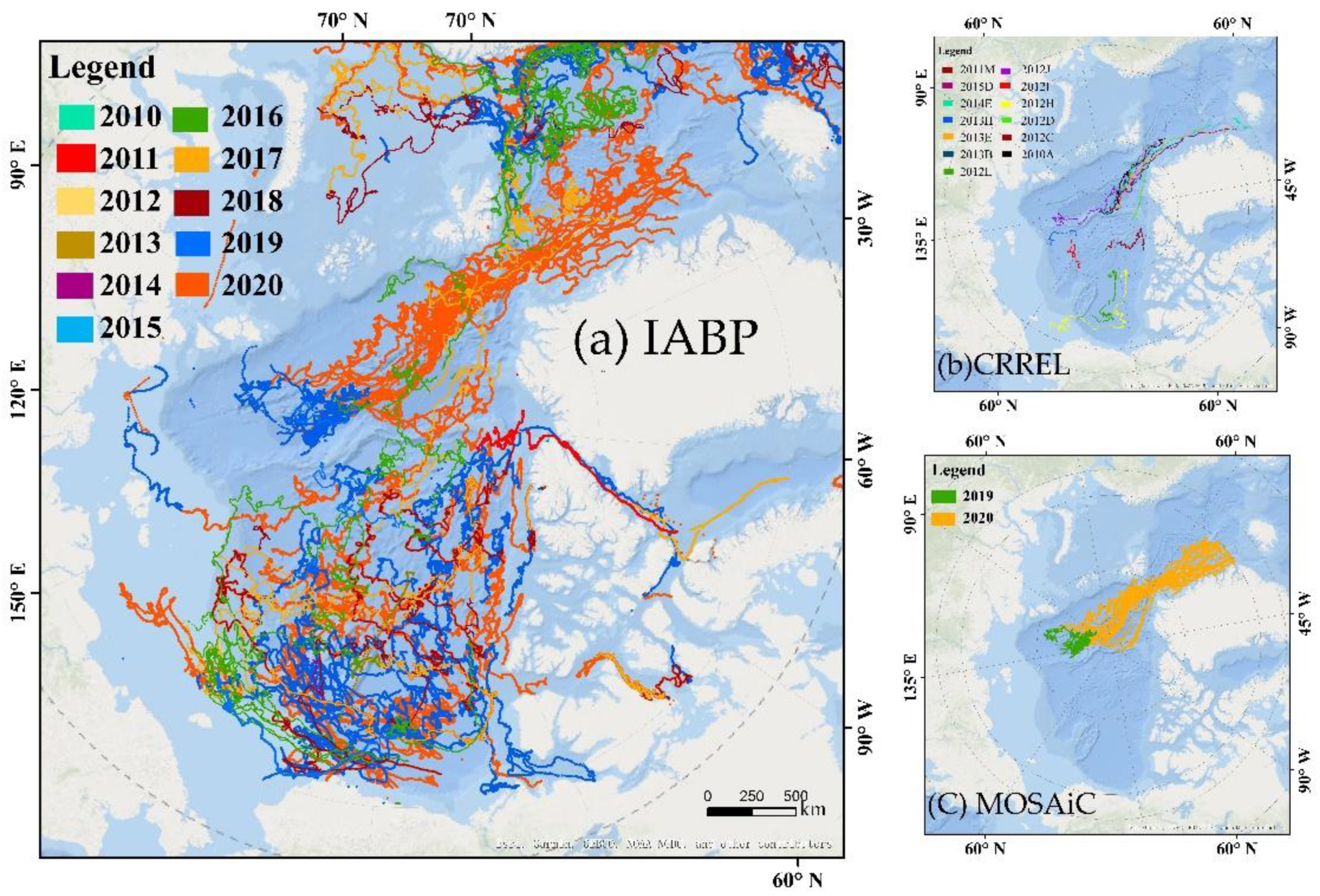
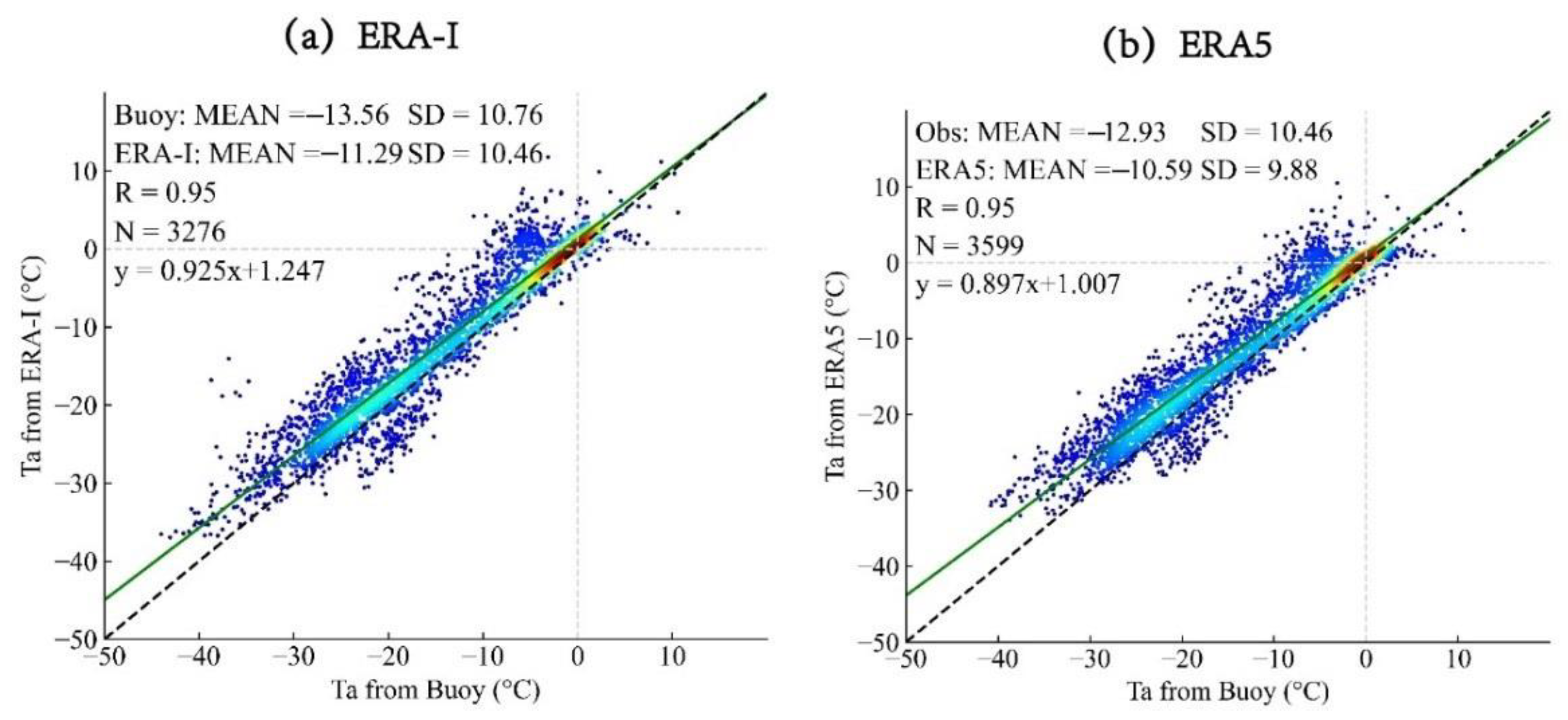
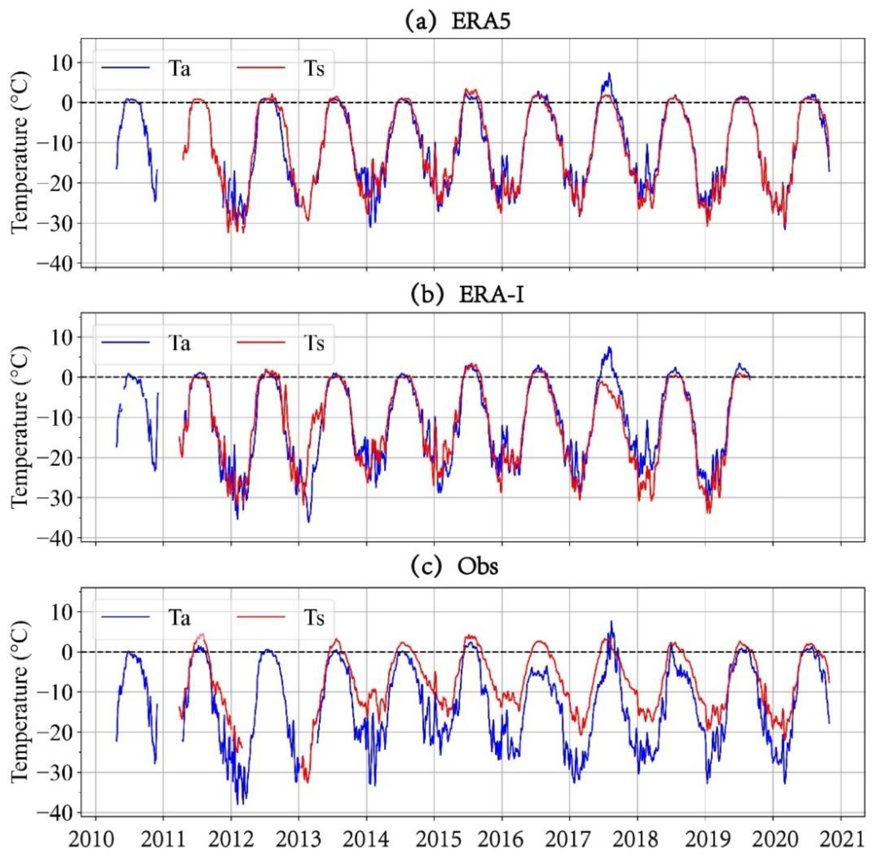
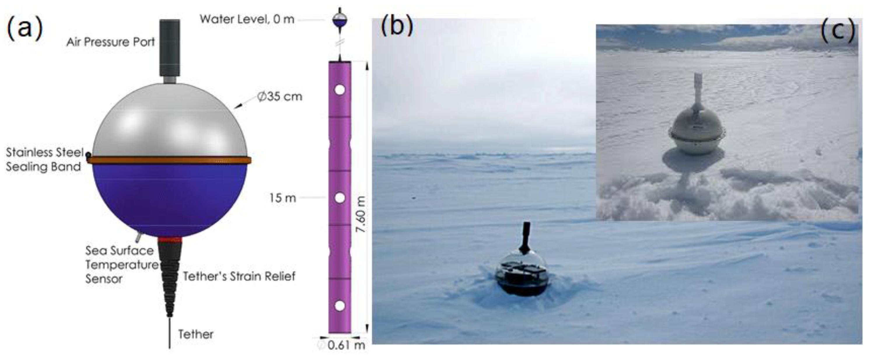
In this study, we focused on two temperature variables from both ERA-I and ERA5, namely, the 2-m air temperature (Ta) and the surface temperature (Ts). Ta was calculated by interpolating between the lowest model level and the Earth’s surface, and by making use of the same profile functions as in the parametrization of the surface fluxes [39]. Ts is the temperature of the surface cover. It is the theoretical temperature that is required to satisfy the surface energy balance. It represents the temperature of the uppermost surface layer, which has no heat capacity and thus can respond instantaneously to changes in the surface fluxes. We evaluated the performances of these two reanalysis datasets over the Arctic sea ice floes, using in-situ observations from 910 buoys (676 buoys for Ts and 234 buoys for Ta) during 2010–2020, which represents the largest spatial and longest temporal coverage ever reported. The data and methods are introduced in Section 2. The evaluation results for ERA5 and ERA-I are presented in Section 3. The discussions and conclusions are presented in Section 4 and Section 5, respectively.
Table 1. Assessments of the temperature variables in the ERA series reanalysis datasets over the cold regions in the Northern Hemisphere in the previous studies. The research methods for these studies were similar and can be used to compare the reanalysis datasets with in-situ measurements.
ResearchersPeriodStudy AreaIn-Situ MeasurementsReanalysis DataParametersConclusions
Tjernström & Graversen (2009) [40]1997–1998Beaufort SeaSoundingsERA-40Temperature at atmospheric boundary layerWarm bias (0.5–1.0 °C)
Lüpkes et al. (2010) [41]1996/8, 2001/8, and 2007/8Cruise tracks of RV Polarstern in Arctic OceanSensors on board (30 m)ERA-ITemperature at the second-lowest model level (height ≈ 38 m)Warm bias (1.5–2 °C)
Jakobson et al. (2012) [25]2007/4–2007/8Central ArcticSoundingsERA-IAir temperature profile (0–890 m)Warm bias (up to 2.0 °C)
Gao et al. (2014) [42]1979–2010Tibetan PlateauMeteorological stationsERA-I2 m temperatureWarm biases (up to 10.5 °C)
Lindsay et al. (2014) [20]1981–2010Arctic LandLand stationsERA-I2 m temperatureWarm bias in winter (up to 0.5 °C) and cold bias in summer (−0.7 °C)
Rapaić et al. (2015) [43]1958–2010Canadian Arctic LandLand stationsERA-40 and ERA-I2 m temperatureWarm biases for both ERA-I and ERA-40
Wang et al. (2019) [35]2010–2016Arctic Ocean16 BuoysERA-I and ERA52 m temperatureWarm biases of 0–8 °C for ERA5 and 0.75–4.4 °C for ERA-I

2. Materials and Methods

2.1. Reanalysis Data

2.1.1. ERA-Interim

The ERA-I reanalysis dataset provides critical information for calibrating proxy records of several atmospheric and surface parameters around the world [30]. It was generated to serve as a bridge between the successful ERA-40 atmospheric reanalysis and future generations of reanalysis provided by the ECWMF [30]. This dataset has been available, but with a two-month delay, from 1979 to 2019, with a spatial resolution of 0.125° and a temporal frequency of 6 h. The ERA-Interim ceased in August 2019 and was succeeded by the ERA5 reanalysis. The 2-m air temperature and skin temperature variables were used in the comparisons in this study. The dataset was obtained (for free but requiring registration) from the following address: https://www.ecmwf.int/en/forecasts/datasets/reanalysis-datasets/era-interim (accessed on 2 December 2020).

2.1.2. ERA5

ERA5 is the latest climate reanalysis dataset released by the ECMWF and is a successor to the ERA-I dataset [31]. The ERA5 dataset provides atmospheric and surface parameters from 1950 to the present. The most substantial improvements compared to the ERA-Interim include better availability and a higher temporal resolution (hourly) [34]. Compared to ERA-I, ERA5 also provides more parameters. ERA5 benefits from several upgrades, including the observation operators, and more importantly, a new data assimilation strategy (Integrated Forecast System (IFS) Cy41r2). The 2-m air temperature and skin temperature variables were used in the comparisons in this study. The dataset was obtained (for free but requiring registration) from the following website: https://www.ecmwf.int/en/forecasts/datasets/reanalysis-datasets/era5 (accessed on 2 December 2020).

2.2. Buoy Observations

2.2.1. International Arctic Buoy Program

The International Arctic Buoy Program (IABP) is a coordinating program for autonomous buoy activities targeting numerous objectives in the Arctic [44]. The operational area of the IABP is the entire Arctic Ocean, including its marginal seas. The Argos system was implemented to transmit the in-situ observation data. There are hundreds of autonomous buoys and drifting stations under normal operating conditions, and these instruments were deployed every year at the North Pole, in the Beaufort Gyre, and at other locations of opportunity. Most of the instruments in the IABP can provide surface temperature time series data, but it is hard to get access to the vertical temperature profiles due to a lack of temperature chain sensors (https://iabp.apl.uw.edu/index.html (accessed on 15 November 2020)). It should be noted that the surface temperature is measured at the bottom of the buoy’s hull. If the buoy is floating, then the reported temperature is the sea surface. If the buoy is frozen in ice, or sitting on top of ice, then the reported temperature is the surface temperature of the ice. The freezing temperature of sea water is about −1.8 °C, so temperature readings below this indicate ice temperatures. In addition to surface temperature, there are other basic parameters in each buoy file, for example, the buoy ID, year, hour, min, DOY, POS_DOY (the day of the year to the decimal minute of the reported position), latitude, and longitude. As shown in Figure 1a, the IABP buoy dataset used in this study was the daily updated level-1 in the Arctic during 2011/1–2020/10 and provided records at hourly intervals. We selected 730 buoys deployed in different regions of the Arctic (North of 70° N), including 589 buoys for surface temperature and 141 buoys for air temperature.

2.2.2. MOSAiC

The Multidisciplinary Drifting Observatory for the Study of Arctic Climate (MOSAiC) program was a one-year-long (September 2019–October 2020) expedition in the Central Arctic (https://mosaic-expedition.org/expedition/ (accessed on 10 December 2020)). It was the largest international Arctic research initiative in history, was organized around broad science questions, and was mainly motivated by the dramatic changes in the Arctic climate system over the last few decades [45]. In order to obtain the needed observations, MOSAiC included the construction of a distribution network with its outer boundary defined by a set of nodes at the four corners of a ~50 km box centered on the Central Observatory. Each node could drift with the ice floe and included a suite of multi-disciplinary, buoy-based measurements, which could be in operation for many years [45]. As shown in Figure 1b, we utilized observations from 167 buoys from 2019/10 to 2020/12, including 87 buoys for surface temperature and 80 buoys for air temperature. Both temperatures were recorded at half-hour intervals.

2.2.3. CRREL

The overarching goal of the Cold Regions Research and Engineering Laboratory (CRREL)-Dartmouth Mass Balance Buoy Program was to be a component of a sustainable Arctic observation network. These buoys were equipped with oceanic and atmospheric measurement systems that provided a complete vertical profile of the atmosphere, ice, and upper ocean properties (http://imb-crrel-dartmouth.org/ (accessed on 14 November 2020)). These instruments mainly recorded the hourly air temperature, mean sea level pressure, and vertical temperature profile using a set of temperature sensor chains located in the air, snow, ice, and the upper ocean [35]. Based on the temperature profile, with a 2 cm interval between adjacent sensors, it is easy to obtain the boundary positions between the air, snow, ice, and ocean. A total of 13 buoys were selected for use in this study, which were also utilized in a previous study [35]. The trajectories of these buoys during 2010/4–2016/10 are shown in Figure 1c.

2.3. Methods

As was mentioned above, the observations utilized in this study came from three different international buoy programs with various data record formats and observation parameters. For convenience, we transformed the formats of the different buoy datasets into the same format as the ERA reanalysis data. First, we processed the different buoy observations to generate data with identical information, including buoy ID, date, location, air temperature, and surface temperature. This is efficient for further extracting the buoy observation records and matching them with the ERA5 and ERA-I temperature data. Second, using the programming tools, we automatically matched and extracted the air/surface temperature and geo-location information from the buoy observations and the reanalysis data when the corresponding date and time in the two datasets were the same.
Since the ERA-I and ERA5 reanalysis datasets were gridded as 0.25° and 0.125°, respectively, and the observations from the buoys were collected based on single coordinates, we assigned the temperature record of the buoy observations to its corresponding grid point in the reanalysis data based on the principle of the nearest distance to generate a set of matching pairs between the buoy observations and the reanalysis data. Finally, 1,938,483 pairs from IABP, 431,874 pairs from MOSAiC, and 90,141 pairs from CRREL were extracted and analyzed in this study.

3. Results

3.1. Evaluation of 2-m Air Temperature (Ta)

3.1.1. Long-Term Variations

Figure 2a shows the time series of the daily mean Ta from the ERA5 (blue), ERA-I (red), and the buoy observations (black), averaged from all of the buoys’ trajectories during 2010–2020. All three datasets exhibit similar inter-annual and seasonal cycles. During January, the temperature was the lowest, and then, it gradually rose from February to June, with a continuous high temperature near 0 °C through the summer. Beginning in September, the temperature dropped significantly to around −30 °C until the end of the year, leading to a clear seasonal Ta cycle.
As shown in Figure 2b, the biases for both the ERA5 and the ERA-I were generally positive but were different in different years. For example, both biases were up to 10 °C during the summer of 2017 when the Ta values were largely above 0 °C but were mostly less than 5 °C. It is noteworthy that both reanalysis datasets exhibited cold biases (as large as −5 °C) in 2015 and 2019. The differences between the ERA-I and ERA5 exhibited clear interannual and seasonal variations. In general, the Ta from the ERA5 was 0.21 °C warmer than that from the ERA-I.
Large differences between the ERA-I and ERA5 have also been found in previous buoy comparisons, reaching more than 4 °C. Further comparisons have indicated that the biases were larger when the air temperature was less than −25 °C [35].
The biases of greater than 10 °C were checked in detail, and it was found that they mainly occurred during 2017–2018 when only 21 IABP buoys were available for these two years, and that no observations were available from CRREL (available during 2010–2016) and MOSAiC (available during 2019–2020). Therefore, the limitation caused by the number of buoys may have caused the larger biases, which indicated that a large number of buoys and cross buoy programs would increase the reliability of the comparisons. In our study, the available period for ERA-I was during 2010–2019, which stopped to update since August 2019. Whereas, ERA5 is an updated version with a longer time series of 2010–2020. The slightly different period for the ERA-I and the ERA5 may introduces biases too. The different temporal and spatial scales of the reanalysis datasets and the buoy observations, i.e., gridded data (0.125° and 0.25°) for the reanalysis and trajectory measurements for the buoys, also introduced biases into the comparisons.
Figure 3a shows a scatter plot of the daily mean Ta from the ERA-I and buoy observations during 2011–2019, with 3276 matching pairs. The Ta of the ERA-I and buoy observations generally agreed well, and the correlation coefficient was 0.95. The multi-year mean Ta of the buoy observations was −13.56 ± 10.76 °C and that of the ERA-I was −11.29 ± 10.46 °C, which indicates that the ERA-I shows a warm bias of 2.27 ± 3.33 °C. Similar to Figure 3a, the scatter plot of the daily mean Ta from the ERA5 during 2010–2020 is shown in Figure 3b, with a total of 3599 matching pairs and a correlation coefficient of 0.95. The multi-year mean Ta was −12.93 ± 10.46 °C for the buoy observations and −10.59 ± 9.88 °C for the ERA5. These comparisons indicate that the ERA5 exhibited a slight warmer bias of 2.34 ± 3.22 °C than the ERA-I.
As shown in Figure 3, the Ta values from both the reanalysis datasets were mostly distributed close to the 1:1 line, and they generally exhibited warmer trends when below 0 °C. The lower the temperatures, the larger the warm biases. As shown in Table 2, if the 10 °C temperature intervals are considered, the results show that the ERA5 exhibited warmer pattern in all of the intervals, except for 0–10 °C. This is consistent with our conclusion based on the comparison of the total biases of the ERA-I and ERA5.

3.1.2. Seasonal Cycles

Figure 4 shows the monthly mean biases of the Ta between the reanalysis datasets and the buoy observations. In general, the biases were warm for both ERA-I and ERA5 in all of the months, and the largest biases occurred in April (3.02 ± 2.79 °C for ERA-I and 3.73 ± 2.84 °C for ERA5; Table 3). The biases were relatively small in August, September, October, and November, i.e., less than 2 °C. The monthly differences between the ERA5 and ERA-I exhibited seasonal variations, with negative differences occurring in the warm season (July, August, and September) and positive differences occurring in the other months. The largest negative difference was −0.36 ± 0.80 °C in July, and the largest positive bias was 1.17 ± 1.79 °C in March (Table 3).
Figure 5 shows the calendar diagram of the multi-year mean daily Ta bias between the buoy observations and the two reanalysis datasets and the biases between ERA5 and ERA-I. Compared with the buoy observations, both reanalysis datasets exhibited clear and overall warm biases during the entire year, with only one day showing a cold bias for ERA-I and four days showing cold biases for ERA5. For ERA-I, the largest bias was 6.23 °C, with 80.5% of the bias exceeding 2 °C, and for ERA5, the largest bias was 4.85 °C, with 79.5% of the bias exceeding 2 °C. ERA5 exhibited much warmer daily biases from January to June, especially in February and April.
Based on Table 3, both the reanalysis datasets and buoy observations reveal that the maximum monthly temperature occurred in July (1.40 ± 1.37 °C for ERA5, and 1.76 ± 1.70 °C for ERA-I, and −0.55 ± 2.58 °C for buoy). The smallest monthly bias was 1.36 ± 2.51 °C in September for ERA5 and 1.72 ± 2.62 °C in October for ERA-I. Otherwise, the largest bias for ERA5 occurred in April (3.73 ± 2.84 °C), and that of the ERA-I-buoy occurred in July (3.12 ± 2.44 °C). For both reanalysis methods, the root mean square error (RMSE) values were nearly double in January, February, and March, which indicates larger bias variations in these rather cold months compared with other months.
Our assessments of the 2-m air temperature are highly consistent with the results of a previous study, that is, 0.75–4.4 °C and 0.75–8.0 °C warm biases for ERA-I and ERA5, respectively, based on 13 CRREL buoys in the Arctic during 2010–2016 [35]. In addition, other previous studies have shown that the warm biases in the reanalysis data widely occurred in polar regions under cold conditions when compared with other measurements, including buoys [40,41,43,46,47,48].
Our results are comparable to those of the previous studies shown in Table 1. Numerous comparisons of the 2-m air temperature of the ERA-I have been carried out over the Arctic and in the high mountain regions in the Northern Hemisphere. The results show that warm biases occurred in all of the studies. For the 2-m air temperature of the ERA5, a study in 2019 compared it with in-situ observations from 16 buoys in the Arctic and found a 0–8 °C warm bias, which is consistent with our result (2.34 ± 3.22 °C). However, we used hundreds of buoys (total 234 buoys) compared to the 16 buoys used in the previous study, indicating that our comparisons are more reliable.
The accuracy of the assessment of the 2-m air temperature may be related to two factors. First, it is affected by the height of the air temperature sensor on the buoy, which is usually lower than 2 m for the buoys. Another reason is the poorly modelled near-surface inversion of the reanalysis datasets [40,41,49], which may be connected with the strong turbulent diffusivity in the boundary layer under stable conditions [49], or the simple representation of the sea ice thickness as 1.5 m and the snow-free assumption over the sea ice in the Arctic [35,47].

3.2. Evaluation of Surface Temperature (Ts)

3.2.1. Long-Term Variations

Figure 6a clearly depicts the generally good agreement between the annual Ts cycles from ERA5 (blue), ERA-I (red), and the buoy observations (black). The daily mean Ts for both the ERA5 and ERA-I ranged from −35 °C in winter to nearly 5 °C in summer during 2011–2020. Compared with the buoy observations, both reanalysis methods exhibited significant cold biases, except for ERA5 and ERA-I in 2013 (Figure 6b). The biases exhibited clear seasonal variations, with some larger than −10 °C in winter and close to 0 °C in summer. The differences between ERA5 and ERA-I changed significantly during different years. In particular, they were greater than 5 °C in 2013, 2017, 2018, and 2019.
A total of 3060 and 3487 matching pairs for ERA-I and ERA5, respectively, were used for the comparisons of the daily mean Ts (Figure 7a,b). Based on the scatter plots, both reanalysis methods exhibited significant cold biases, and the biases were larger when the surface temperature was low. Furthermore, as shown in Table 4, if the 10 °C temperature intervals are considered, the ERA-I was closer to the buoy observations in the cold environments (lower than −20 °C), while the ERA5 performed better in the −10–0 °C and 0–10 °C intervals.

3.2.2. Seasonal Cycles

Figure 8 shows the seasonal changes in the biases between the ERA5, ERA-I, and buoy observations. Both the ERA5 and ERA-I exhibited cold biases for all of the months when compared with the buoy observations. The Ts from ERA5 exhibited warmer biases for most of the period, except for March and April, when compared with ERA-I. The cold biases (greater than −6 °C) usually occurred in the cold season (November, December, January, and February), and the largest bias occurred in December, exceeding −10 °C for both reanalysis datasets. However, in the warm summer, the biases were usually rather small, less than −3 °C from April to October.
Figure 9 shows a calendar diagram of the multi-year mean daily Ts biases for ERA5 and ERA-I. Compared with the buoy observations, there was a notable cold bias for the entire year, except for 8 days in May for ERA-I and 18 days during May and June for ERA5. For ERA-I, the maximum bias was −10.81 °C, and 46% of the biases of the time series were greater than −4 °C. For ERA5, the maximum bias was −10.67 °C, and the proportion of the biases greater than −4 °C was also 46%. In addition, the seasonal cycles of the daily cold bias were obvious for both reanalysis datasets, which illustrates the relatively larger bias during the cold seasons and the relatively smaller bias during the warm seasons.
As shown in Table 5, the Ts from both reanalysis datasets exhibited seasonal cycles, and the lowest monthly mean temperatures occurred in January, reaching −24.06 °C for ERA5 and −25.26 °C for ERA-I. In July, the mean monthly temperature increased to the maximum and exceeded 0 °C for both reanalysis datasets. The monthly differences between the ERA5 and ERA-I were small, from −0.54 °C to 1.49 °C. The largest difference was 1.49 ± 2.26 °C in November and the smallest was −0.08 ± 2.98 °C in April. The Ts values from ERA5 were higher than those from ERA-I during most of the months, except for March and April.
Compared with the buoy observations, the biases in all the months were negative, ranging −0.54 to −9.90 °C for ERA5 and from −1.29 to −11.18 °C for ERA-I, and they were larger in the cold season than in the warm season. The RMSE distribution also illustrates the seasonal variations, which were about five to ten times larger in the cold seasons (maximum of 10.33 °C for ERA5 and 11.59 °C for ERA-I) compared with the warm seasons (minimum of 1.48 °C for ERA5 and 2.01 °C for ERA-I).

4. Discussion

4.1. Comparisons of Ta and Ts

Basically, Ta and Ts exhibited similar and reasonable seasonal cycles for both ERA5 and ERA-I. As shown in Figure 10a, b, the differences between Ta and Ts were small during most of the time series, except for in the spring of 2013 and the summer of 2017. The maximum daily differences in Ta and Ts for ERA5 were 15.05 °C and −15.95 °C, respectively, while for ERA-I they were 22.81 °C and −18.14 °C during the entire time series.
When compared with the buoy observations (Figure 10c), Ta and Ts both exhibited similar patterns with varying amplitudes in both summer and winter. Overall, Ts was generally warmer than Ta, and the differences were as large as 10 °C in winter and 5 °C in summer. The reason for the warmer Ts values may be the monitoring location of the surface temperature sensor on the buoy, which is usually located at the bottom of the IABP buoy’s hull. When the buoy is frozen into the sea ice, the values recorded by the surface temperature sensor are in fact the ice’s inner temperature, which is warmer than Ta because of the thermal insulation effect of the snow cover and the sea ice. Due to this, the Ts recorded by the buoys may overestimate the surface temperature, which may be responsible for the large cold Ts bias from both the ERA5 and ERA-I. Therefore, the cold Ts biases evaluated in Section 3.2.2 may be overestimated.

4.2. Impact of Snow on Ice Surface Temperature

For a typical IABP buoy, the radius of the operation sphere is 35 cm, and the surface temperature sensor is located near the bottom of the buoy (Figure 11a). When the buoys were distributed over sea ice in the Arctic, the surface temperature sensor may be frozen into the ice surface layer or even covered by the snow layer. Usually the surface temperature did not measure the inner ice temperature exactly 35 cm below ice surface because the ice stress can arch the buoy up and make the surface temperature sensor closer to the ice surface (Figure 11b,c). Therefore, the maximum depth of the sensor was no more than 35 cm, but the real depth was hard to determine. When the ice surface was snow free, the measured temperature was regarded as the ice surface temperature. However, when snow was present, the measured temperature was affected by the large heat insulation effect of the snow.
The snow simplification issues in the ERA-I and ERA5 parameterization also caused biases (reported to be 5–10 °C), and simplified consistent snow and ice parameters were applied in the assimilation model, for example, setting the sea ice thickness to 1.5 m and the snow thickness to zero [46]. Due to the lack of real snow thickness measurements and products over the Arctic sea ice, it was hard to quantify the snow effect on the temperature measurements along the buoy drift trajectories; therefore, we only discuss the snow’s effect for different snow thickness ranges under different air temperature conditions.
If we assume the thermal conductivity of snow to be 0.31 W/m K [51], the typical temperature gradient of snow would be 0.1–0.5 °C/cm [52]. We used mean gradients (0.2 °C/cm, 0.35 °C/cm, 0.5 °C/cm, and 0.65 °C/cm for the air temperature cases of −10 °C, −20 °C, −30 °C, and −40 °C, respectively) to estimate the possible temperature effect caused by the snow cover. If snow covered on the ice surface was 5 cm thick, then the biases of ice surface temperature between the reanalyzes and the IABP measurements were overestimated by1 °C for the −10 °C case and 3.25 °C for the −40 °C case. The same calculations were applied to other cases and the detailed results are presented in Table 6. As we can conclude from Table 6, the lower the temperature and the deeper the snow thickness, the bigger the overestimation caused by snow cover.

4.3. Bias Variations in the Different SIC Ranges

The buoys drifted in the different SIC (sea ice concentration) regions due to the growth or retreat of the sea ice extent and the ocean currents. The different SICs had different percentages of water and ice, which dominated the heat exchange between the atmosphere and ocean. Therefore, the assessment of the Ta and Ts may be significantly affected by the SIC, especially when a large grid cell of 12.5–25 km was used in the analysis datasets. For Ta (Figure 12a), 11–19% of the buoys were distributed in regions with SICs ranging from 0 to 20%, which is regarded as open water. In addition, 76–86% of the buoys drifted in areas with SICs of 80–100%, which is regarded as frozen on ice. These two situations accounted for more than 95% of the buoy positions in this study. It is obvious that the biases of the Ta became larger when the buoy locations had SICs of 20–80% because large uncertainties existed when the surface type within a single grid cell was not homogeneous but was a mixture of water and ice.
For the Ts from the ERA-I and ERA5 (Figure 12b), the distribution of the biases relative to the different SIC values was significantly larger in the high SIC range (80–100%), in which the buoys are believed to be frozen in the ice. Therefore, the larger biases may be related to the snow cover on the ice. As we discussed above, the snow cover would significantly increase the ice surface temperature because of its large heat insulation effect. Therefore, the surface temperature was sensitive to the surface conditions in the Arctic.

4.4. Bias Variations between Different Buoy Projects

For the ERA5 data (Table 7), the total number of matching pairs was 778,331 for the Ta evaluation, among which 68% were for IABP, 22% were for MOSAiC, and 10% were for CRREL. However, the total number of matching pairs was 1,610,662 for the Ts evaluation, among which 84% were for IABP and 16% were for CRREL. Therefore, the IABP was the main source of the buoy observations used in this study. The bias of Ta between the reanalysis and buoy observations was the smallest for MOSAiC (0.12 ± 1.76 °C), followed by CRREL (2.25 ± 2.49 °C), and was the largest for IABP (3.27 ± 4.69 °C). The RMSE values follow the same sequence, i.e., 1.76 °C, 3.36 °C, and 5.72 °C for MOSAiC, CRREL, and IABP, respectively. The evaluated Ts bias was −3.33 ± 3.08 °C for MOSAiC and −4.43 ± 4.27 °C for IABP. The smallest bias and RMSE values for both the Ta and Ts of the ERA5 were for MOSAiC. In addition to having fewer matching pairs than IABP, the reason for this may also be related to the improved equipment and sensors compared with the other two buoy projects, which were conducted in recent years (2019–2020).
For the ERA-I Ta evaluation (Table 8), the total number of matching pairs was 71,505, among which 82% were for IABP and 18% were for CRREL. The total number of matching pairs was 160,071 for the Ts evaluation. Generally, the number of buoy observations used for the ERA-I was ten times less than the number used for the ERA5. The Ta from the ERA-I exhibited a warm bias of 1.05 ± 3.60 °C for IABP and 1.60 ± 2.83 °C for CRREL. The RMSEs were 3.75 °C and 3.25 °C for IABP and CRREL, respectively.

5. Conclusions

When monitoring the rapid climate warming in the Arctic, in-situ measurements, remote sensing products, and reanalysis datasets are the primary datasets used by the scientific community. The in-situ measurements, including drifting buoys, offer the most accurate atmospheric and oceanic data, but are limited by their sparse distributions. Reanalysis datasets are of great significance to filling the unobserved data gaps on temporal and spatial scales, but they need to be validated before being used for further research. In this study, we evaluated the performance of the 2-m air temperature (Ta) and the surface temperature (Ts) in the Arctic produced from the ERA-I and ERA5 reanalysis datasets based on in-situ observations from 910 drifting buoys monitored by three international buoy programs during 2010–2020. The buoy observations used in this study covered the largest area with the longest period ever reported in research related to the Arctic.
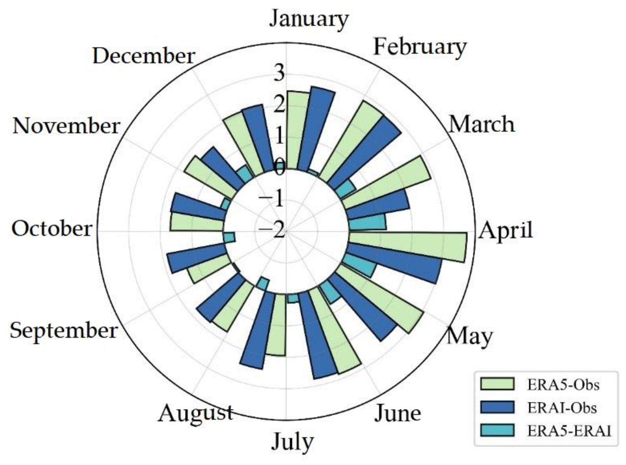
First, the Ta from the reanalysis datasets exhibited similar seasonal cycles and high correlation coefficients of 0.95 when compared with the buoy observations. The Ta from the ERA-I exhibited a warm bias of 2.27 ± 3.33 °C, while the Ta from the ERA5 exhibited a warmer bias of 2.34 ± 3.22 °C based on the comparisons of more than 3000 daily matching pairs. The warm Ta biases exhibited monthly variations with the maximum occurring in April. However, the smaller warm biases occurred in the warm season (June, July, and August). Negative biases were found to occur on only one day for ERA-I and four days for ERA5 in multi-year mean daily biases; therefore, warm biases occurred throughout most of the year.
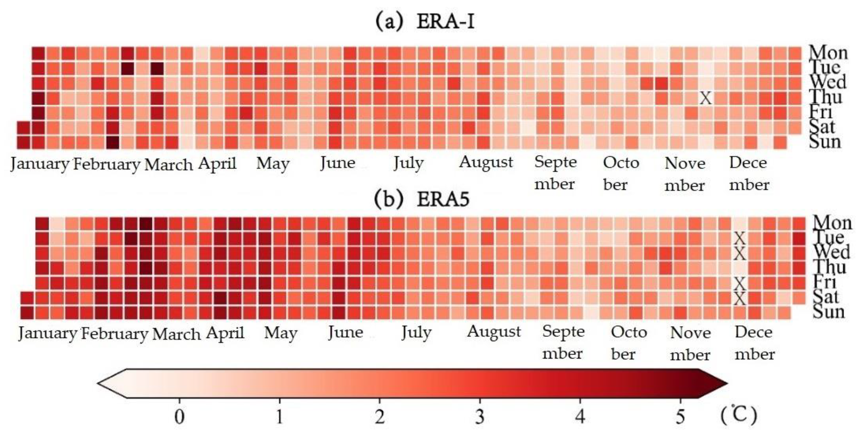
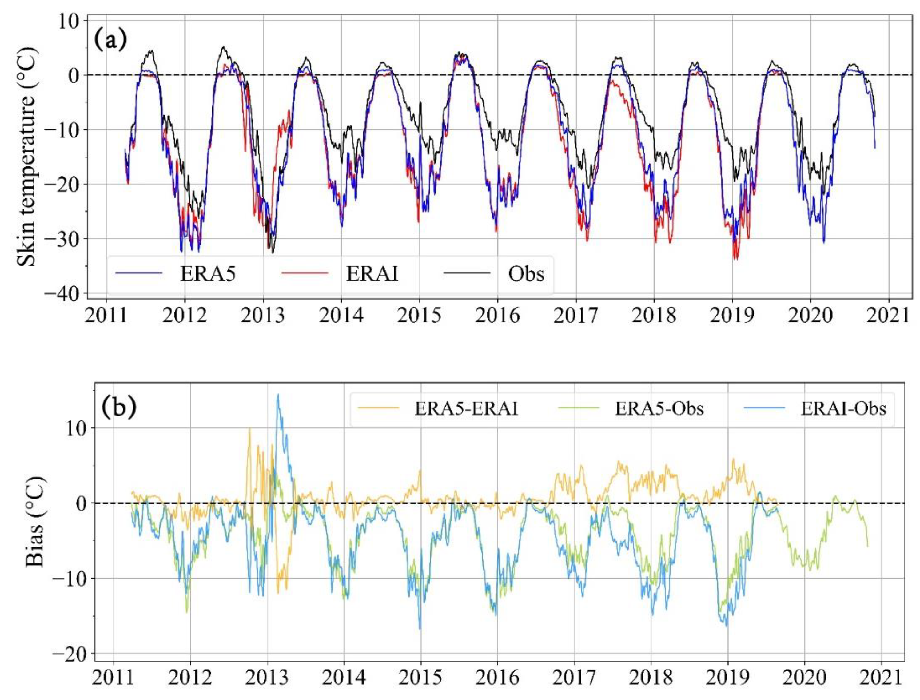
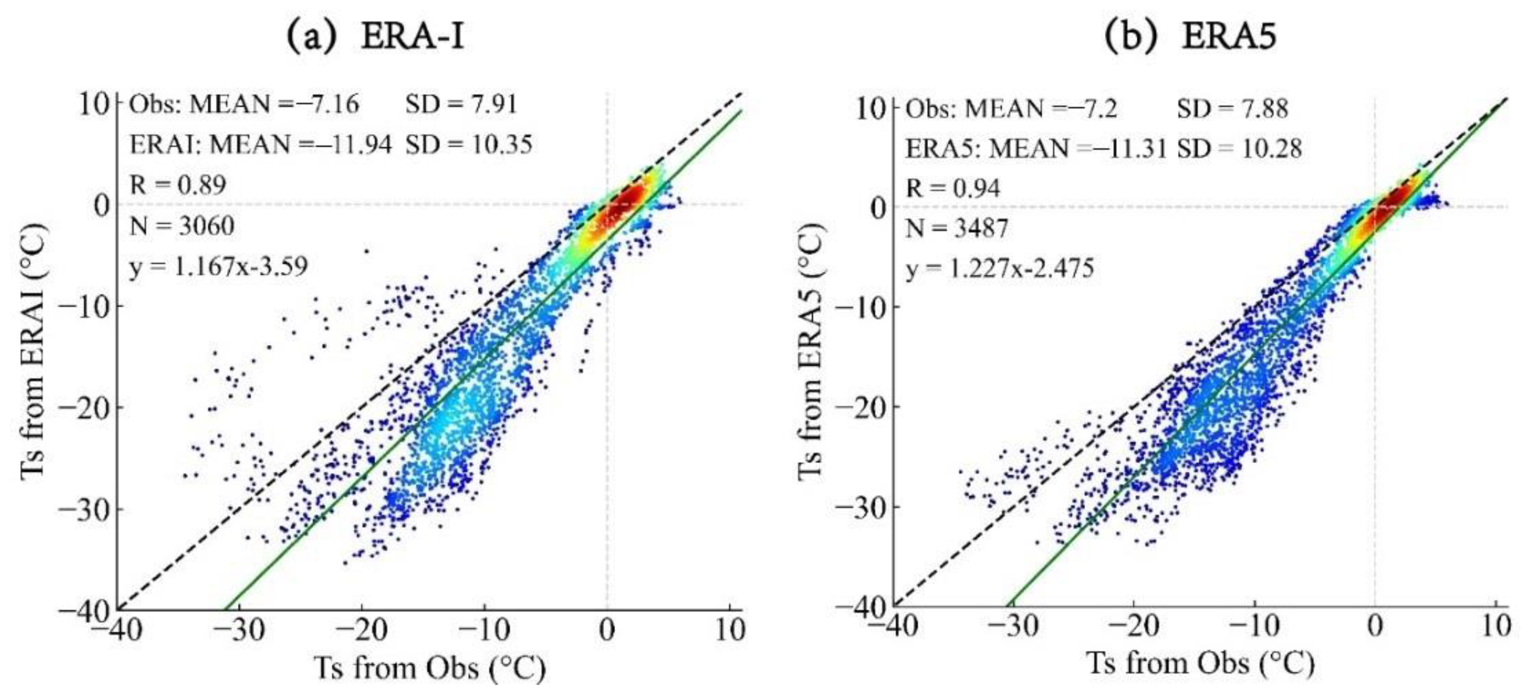
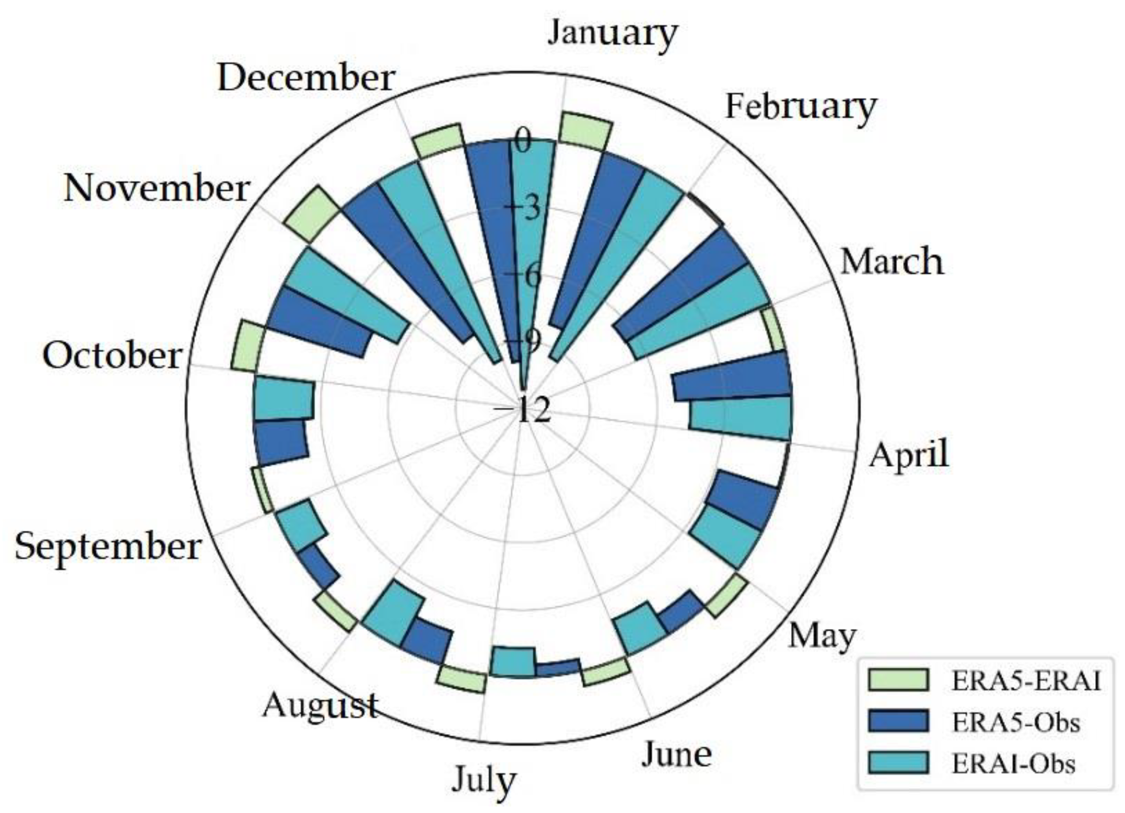
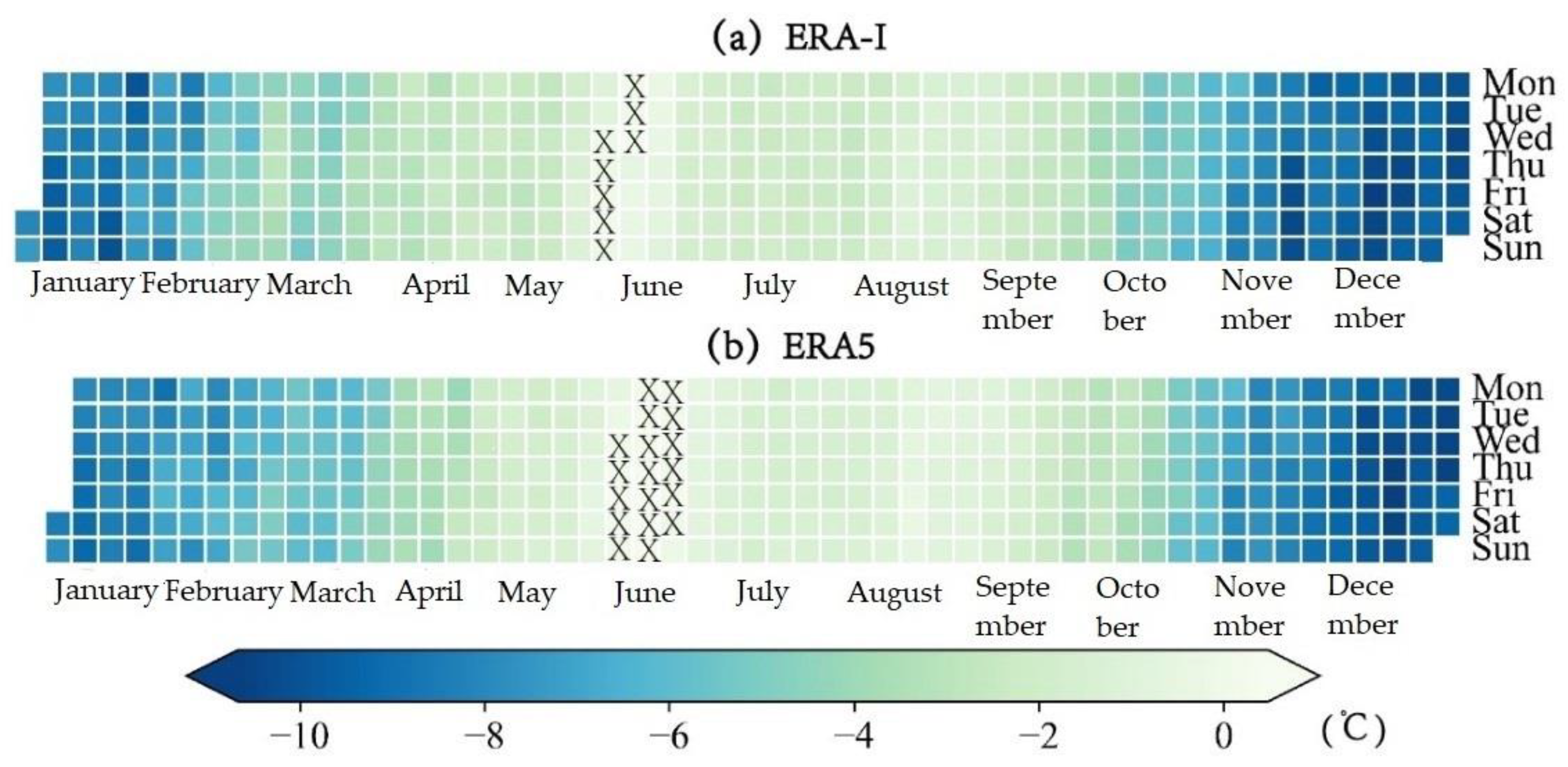
Second, the Ts from ERA-I and ERA5 both exhibited similar variation patterns, but the cold bias from ERA-I was larger, especially in winter. The largest cold biases of the ERA-I and ERA5 were up to −10 °C for every winter during 2011–2020. Generally, the cold biases were larger when the temperature was lower. For the monthly comparison, the largest biases occurred in December. However, the biases were normally less than −3 °C during April–October. The warmer Ts may be related to the location of the surface temperature sensor on the buoy, which is located near the bottom of the IABP buoy’s hull and may be affected by the snow cover. Based on this point, the cold Ts biases of the ERA-I and ERA5 are probably overestimated.
The small quantity of buoys may have caused the larger biases during 2016–2018, which indicated that enough buoys and cross buoy programs would increase the reliability of validations. The different temporal and spatial scales of the reanalysis datasets and buoy observations also introduced biases into the comparisons. In the future, more unmanned buoys and improved sensor technology will enhance the span and accuracy of the in-situ observations. The combination of enough observations and improved assimilation methods will improve the quality of the reanalysis datasets.

Author Contributions

Y.Y. processed and analyzed the data; Y.Y. and W.X. wrote the manuscript; Y.Y. and J.Z. designed the experiments; Z.Z. and X.C. discussed the results; J.Z. and F.H. investigated the results, revised the manuscript, and supervised this study. All authors provided substantial input to the interpretation of the results. All authors have read and agreed to the published version of the manuscript.

Funding

This work was supported by National Natural Science Foundation of China (Grant No. 41976214), National Key Research and Development Program of China (2016YFC1402704) and Innovatiom Group Project of Southern Marine Science and Engineering Guangdong Laboratory (Zhuhai) (No. 311021008).

Acknowledgments

We greatly thank ECWMF for providing ERA-I (https://www.ecmwf.int/en/forecasts/datasets/reanalysis-datasets/era-interim, accessed on 14 November 2020) and ERA5 (https://www.ecmwf.int/en/forecasts/datasets/reanalysis-datasets/era5, accessed on 14 November 2020) reanalysis. We also thank IABP (https://iabp.apl.uw.edu/index.html, accessed on 14 November 2020), MOSAiC (https://mosaic-expedition.org/expedition/, accessed on 14 November 2020) as well as CRREL (http://imb-crrel-dartmouth.org/, accessed on 14 November 2020) for providing buoy observations, and we truly appreciate reviewers for their valuable comments.

Conflicts of Interest

The authors declare no conflict of interest.

References

  1. Serreze, M.C.; Barry, R.G. Processes and impacts of Arctic amplification: A research synthesis. Glob. Planet. Chang. 2011, 77, 85–96. [Google Scholar] [CrossRef]
  2. Cohen, J.; Screen, J.A.; Furtado, J.C.; Barlow, M.; Whittleston, D.; Coumou, D.; Francis, J.; Dethloff, K.; Entekhabi, D.; Overland, J.; et al. Recent Arctic amplification and extreme mid-latitude weather. Nat. Geosci. 2014, 7, 627–637. [Google Scholar] [CrossRef] [Green Version]
  3. Bekryaev, R.V.; Polyakov, I.V.; Alexeev, V.A. Role of polar amplification in long-term surface air temperature variations and modern Arctic warming. J. Clim. 2010, 23, 3888–3906. [Google Scholar] [CrossRef]
  4. Graham, R.M.; Cohen, L.; Petty, A.A.; Boisvert, L.N.; Rinke, A.; Hudson, S.R.; Nicolaus, M.; Granskog, M.A. Increasing frequency and duration of Arctic winter warming events. Geophys. Res. Lett. 2017, 44, 6974–6983. [Google Scholar] [CrossRef] [Green Version]
  5. Boisvert, L.; Stroeve, J.C. The Arctic is becoming warmer and wetter as revealed by the Atmospheric Infrared Sounder. Geophys. Res. Lett. 2015, 42, 4439–4446. [Google Scholar] [CrossRef]
  6. Overland, J.E.; Wang, M. Recent Extreme Arctic Temperatures are due to a Split Polar Vortex. J. Clim. 2016, 29, 5609–5616. [Google Scholar] [CrossRef]
  7. Francis, J.A.; Chan, W.; Leathers, D.J.; Miller, J.R.; Veron, D.E. Winter Northern Hemisphere weather patterns remember summer Arctic sea-ice extent. Geophys. Res. Lett. 2009, 36, L07503. [Google Scholar] [CrossRef] [Green Version]
  8. Screen, J.A.; Simmonds, I. The central role of diminishing sea ice in recent Arctic temperature amplification. Nature 2010, 464, 1334–1337. [Google Scholar] [CrossRef] [Green Version]
  9. Meehl, G.A.; Chung, C.T.Y.; Arblaster, J.M.; Holland, M.M.; Bitz, C.M. Tropical Decadal Variability and the Rate of Arctic Sea Ice Decrease. Geophys. Res. Lett. 2018, 45. [Google Scholar] [CrossRef]
  10. Onarheim, I.H.; Eldevik, T.; Smedsrud, L.H.; Stroeve, J.C. Seasonal and Regional Manifestation of Arctic Sea Ice Loss. J. Clim. 2018, 31, 4917–4932. [Google Scholar] [CrossRef]
  11. Moore, G.W.K.; Howell, S.E.L.; Brady, M.; Xu, X.; McNeil, K. Anomalous collapses of Nares Strait ice arches leads to enhanced export of Arctic sea ice. Nat. Commun. 2021, 12, 1. [Google Scholar] [CrossRef]
  12. Kwok, R. Arctic sea ice thickness, volume, and multiyear ice coverage: Losses and coupled variability (1958–2018). Environ. Res. Lett. 2018, 13. [Google Scholar] [CrossRef]
  13. Lang, A.; Yang, S.; Kaas, E. Sea ice thickness and recent Arctic warming. Geophys. Res. Lett. 2017, 44, 409–418. [Google Scholar] [CrossRef]
  14. King, J.; Spreen, G.; Gerland, S.; Haas, C.; Hendricks, S.; Kaleschke, L.; Wang, C. Sea-ice thickness from field measurements in the northwestern Barents Sea. J. Geophys. Res. Ocean. 2017, 122, 1497–1512. [Google Scholar] [CrossRef] [Green Version]
  15. Markus, T.; Stroeve, J.C.; Miller, J. Recent changes in Arctic sea ice melt onset, freezeup, and melt season length. J. Geophys. Res. 2009, 114. [Google Scholar] [CrossRef]
  16. Stroeve, J.C.; Markus, T.; Boisvert, L.; Miller, J.; Barrett, A. Changes in Arctic melt season and implications for sea ice loss. Geophys. Res. Lett. 2014, 41, 1216–1225. [Google Scholar] [CrossRef]
  17. Parkinson, C.L. Spatially mapped reductions in the length of the Arctic sea ice season. Geophys. Res. Lett. 2014, 41, 4316–4322. [Google Scholar] [CrossRef] [Green Version]
  18. Curry, J.A.; Schramm, J.L.; Ebert, E.E. Sea ice-albedo climate feedback mechanism. J. Clim. 1995, 8, 240–247. [Google Scholar] [CrossRef]
  19. Tian, Z.; Cheng, B.; Zhao, J.; Vihma, T.; Zhang, W.; Li, Z.; Zhang, Z. Observed and modelled snow and ice thickness in the Arctic Ocean with CHINARE buoy data. Acta Oceanol. Sin. 2017, 36, 66–75. [Google Scholar] [CrossRef]
  20. Lindsay, R.; Wensnahan, M.; Schweiger, A.; Zhang, J. Evaluation of Seven Different Atmospheric Reanalysis Products in the Arctic. J. Clim. 2014, 27, 2588–2606. [Google Scholar] [CrossRef] [Green Version]
  21. Mortin, J.; Svensson, G.; Graversen, R.G.; Kapsch, M.-L.; Stroeve, J.C.; Boisvert, L.N. Melt onset over Arctic sea ice controlled by atmospheric moisture transport. Geophys. Res. Lett. 2016, 43, 6636–6642. [Google Scholar] [CrossRef] [Green Version]
  22. Screen, J.A.; Simmonds, I.; Deser, C.; Tomas, R. The Atmospheric Response to Three Decades of Observed Arctic Sea Ice Loss. J. Clim. 2013, 26, 1230–1248. [Google Scholar] [CrossRef] [Green Version]
  23. Rinke, A.; Maturilli, M.; Graham, R.M.; Matthes, H.; Handorf, D.; Cohen, L.; Hudson, S.R.; Moore, J.C. Extreme cyclone events in the Arctic: Wintertime variability and trends. Environ. Res. Lett. 2017, 12. [Google Scholar] [CrossRef]
  24. Kapsch, M.L.; Skific, N.; Graversen, R.G.; Tjernstrom, M.; Francis, J.A. Summers with low Arctic sea ice linked to persistence of spring atmospheric circulation patterns. Clim. Dyn. 2019, 52, 2497–2512. [Google Scholar] [CrossRef] [PubMed] [Green Version]
  25. Jakobson, E.; Vihma, T.; Palo, T.; Jakobson, L.; Keernik, H.; Jaagus, J. Validation of atmospheric reanalyses over the central Arctic Ocean. Geophys. Res. Lett. 2012, 39. [Google Scholar] [CrossRef] [Green Version]
  26. Cullather, R.I.; Bosilovich, M.G. The Moisture Budget of the Polar Atmosphere in MERRA. J. Clim. 2011, 24, 2861–2879. [Google Scholar] [CrossRef]
  27. Rinke, A.; Dethloff, K.; Dorn, W.; Handorf, D.; Moore, J.C. Simulated Arctic atmospheric feedbacks associated with late summer sea ice anomalies. J. Geophys. Res. Atmos. 2013, 118, 7698–7714. [Google Scholar] [CrossRef] [Green Version]
  28. Moalafhi, D.B.; Evans, J.P.; Sharma, A. Evaluating global reanalysis datasets for provision of boundary conditions in regional climate modelling. Clim. Dyn. 2016, 47, 2727–2745. [Google Scholar] [CrossRef]
  29. Bieniek, P.A.; Bhatt, U.S.; Walsh, J.E.; Rupp, T.S.; Zhang, J.; Krieger, J.R.; Lader, R. Dynamical Downscaling of ERA-Interim Temperature and Precipitation for Alaska. J. Appl. Meteorol. Climatol. 2016, 55, 635–654. [Google Scholar] [CrossRef]
  30. Dee, D.P.; Uppala, S.M.; Simmons, A.J.; Berrisford, P.; Poli, P.; Kobayashi, S.; Andrae, U.; Balmaseda, M.A.; Balsamo, G.; Bauer, D.P.; et al. The ERA-Interim reanalysis: Configuration and performance of the data assimilation system. Q. J. R. Meteorol. Soc. 2011, 137, 553–597. [Google Scholar] [CrossRef]
  31. Hersbach, H.; Bell, B.; Berrisford, P.; Hirahara, S.; Horányi, A.; Muñoz-Sabater, J.; Nicolas, J.; Peubey, C.; Radu, R.; Schepers, D.; et al. The ERA5 global reanalysis. Q. J. R. Meteorol. Soc. 2020, 146, 1999–2049. [Google Scholar] [CrossRef]
  32. Decker, M.; Brunke, M.A.; Wang, Z.; Sakaguchi, K.; Zeng, X.; Bosilovich, M.G. Evaluation of the Reanalysis Products from GSFC, NCEP, and ECMWF Using Flux Tower Observations. J. Clim. 2012, 25, 1916–1944. [Google Scholar] [CrossRef]
  33. Wang, A.; Zeng, X. Evaluation of multireanalysis products with in situ observations over the Tibetan Plateau. J. Geophys. Res. Atmos. 2012, 117. [Google Scholar] [CrossRef]
  34. Urraca, R.; Huld, T.; Gracia-Amillo, A.; Martinez-de-Pison, F.J.; Kaspar, F.; Sanz-Garcia, A. Evaluation of global horizontal irradiance estimates from ERA5 and COSMO-REA6 reanalyses using ground and satellite-based data. Sol. Energy 2018, 164, 339–354. [Google Scholar] [CrossRef]
  35. Wang, C.; Graham, R.M.; Wang, K.; Gerland, S.; Granskog, M.A. Comparison of ERA5 and ERA-Interim near-surface air temperature, snowfall and precipitation over Arctic sea ice: Effects on sea ice thermodynamics and evolution. Cryosphere 2019, 13, 1661–1679. [Google Scholar] [CrossRef] [Green Version]
  36. Luo, B.; Minnett, P.J. Evaluation of the ERA5 Sea Surface Skin Temperature with Remotely-Sensed Shipborne Marine-Atmospheric Emitted Radiance Interferometer Data. Remote Sens. 2020, 12, 1873. [Google Scholar] [CrossRef]
  37. Trigo, I.F.; Boussetta, S.; Viterbo, P.; Balsamo, G.; Beljaars, A.; Sandu, I. Comparison of model land skin temperature with remotely sensed estimates and assessment of surface-atmosphere coupling. J. Geophys. Res. Atmos. 2015, 120. [Google Scholar] [CrossRef] [Green Version]
  38. Tsuang, B.-J.; Chou, M.-D.; Zhang, Y.; Roesch, A.; Yang, K. Evaluations of Land–Ocean Skin Temperatures of the ISCCP Satellite Retrievals and the NCEP and ERA Reanalyses. J. Clim. 2008, 21, 308–330. [Google Scholar] [CrossRef]
  39. Ecmwf. Part Iv: Physical Processes. In IFS Documentation CY43R1; ECMWF: Reading, UK, 2016. [Google Scholar]
  40. Tjernström, M.; Graversen, R.G. The vertical structure of the lower Arctic troposphere analysed from observations and the ERA-40 reanalysis. Q. J. R. Meteorol. Soc. 2009, 135, 431–443. [Google Scholar] [CrossRef]
  41. Lüpkes, C.; Vihma, T.; Jakobson, E.; König-Langlo, G.; Tetzlaff, A. Meteorological observations from ship cruises during summer to the central Arctic: A comparison with reanalysis data. Geophys. Res. Lett. 2010, 37. [Google Scholar] [CrossRef] [Green Version]
  42. Gao, L.; Hao, L.; Chen, X.-W. Evaluation of ERA-interim monthly temperature data over the Tibetan Plateau. J. Mt. Sci. 2014, 11, 1154–1168. [Google Scholar] [CrossRef]
  43. Rapaić, M.; Brown, R.; Markovic, M.; Chaumont, D. An Evaluation of Temperature and Precipitation Surface-Based and Reanalysis Datasets for the Canadian Arctic, 1950–2010. Atmos. Ocean 2015, 53, 283–303. [Google Scholar] [CrossRef]
  44. Rigor, I.G.; Clemente-Colón, P.; Hudson, E. The international Arctic buoy programme (IABP): A cornerstone of the Arctic observing network. In Proceedings of the Oceans 2008, Quebec City, QC, Canada, 15–18 September 2008. [Google Scholar]
  45. Multidisciplinary Drifting Observatory for the Study of Arctic Climate Science Plan. 2016. Available online: https://mosaic-expedition.org/expedition/ (accessed on 10 December 2020).
  46. Fréville, H.; Brun, E.; Picard, G.; Tatarinova, N.; Arnaud, L.; Lanconelli, C.; Reijmer, C.; van den Broeke, M. Using MODIS land surface temperatures and the Crocus snow model to understand the warm bias of ERA-Interim reanalyses at the surface in Antarctica. Cryosphere 2014, 8, 1361–1373. [Google Scholar] [CrossRef] [Green Version]
  47. Batrak, Y.; Müller, M. On the warm bias in atmospheric reanalyses induced by the missing snow over Arctic sea-ice. Nat. Commun. 2019, 10, 4170. [Google Scholar] [CrossRef] [PubMed]
  48. Graham, R.M.; Rinke, A.; Cohen, L.; Hudson, S.R.; Walden, V.P.; Granskog, M.A.; Dorn, W.; Kayser, M.; Maturilli, M. A comparison of the two Arctic atmospheric winter states observed during N-ICE2015 and SHEBA. J. Geophys. Res. Atmos. 2017, 122, 5716–5737. [Google Scholar] [CrossRef]
  49. Beesley, J.A.; Bretherton, C.S.; Jakob, C.; Andreas, E.L.; Intrieri, J.M.; Uttal, T.A. A comparison of cloud and boundary layer variables in the ECMWF forecast model with observations at Surface Heat Budget of the Arctic Ocean (SHEBA) ice camp. J. Geophys. Res. Atmos. 2000, 105, 12337–12349. [Google Scholar] [CrossRef] [Green Version]
  50. Centurioni, L.R.; Turton, J.; Lumpkin, R.; Braasch, L.; Brassington, G.; Chao, Y.; Charpentier, E.; Chen, Z.; Corlett, G.; Dohan, K. Global in situ observations of essential climate and ocean variables at the air–sea interface. Front. Mar. Sci. 2019, 6, 419. [Google Scholar] [CrossRef] [Green Version]
  51. Pringle, D.; Eicken, H.; Trodahl, H.; Backstrom, L. Thermal conductivity of landfast Antarctic and Arctic sea ice. J. Geophys. Res. Ocean. 2007, 112, C04017. [Google Scholar] [CrossRef] [Green Version]
  52. Zhao, J.; Zhou, X.; Sun, X.; Cheng, J.; Bo, H.; Chunhua, L. The inter comparison and assessment of satellite sea-ice concentration datasets from the arctic. J. Remote Sens. 2017, 21, 351–364. [Google Scholar]
Figure 1. The trajectories of all of the buoys used in this study, and only those buoys with trajectories to the north of 70° N were utilized. (a) The trajectories of the IABP buoys during 2010–2020; (b) the trajectories of the MOSAiC buoys during 2019–2020; and (c) the trajectories of the CRREL buoys during 2010–2016.
Remotesensing 13 02813 g001
Figure 2. The time series of (a) the daily mean Ta values from the ERA5, ERA-I, and buoy observations and (b) the biases between the ERA5, ERA-I, and buoy observations averaged from all of the buoys’ trajectories during 2010–2020. To obtain a better interpretation of the results, 7-day smoothing was applied to the time series shown here.
Remotesensing 13 02813 g002
Figure 3. Scatter plot of the daily mean Ta from the (a) ERA-I and (b) ERA5. The black dashed line indicates the 1:1 line, and the green line indicates the fitting curve equation of all of the matching pairs.
Remotesensing 13 02813 g003
Figure 4. Rose diagram of the monthly biases of the Ta between the reanalysis datasets and the buoy observations based on the multi-year mean.
Remotesensing 13 02813 g004
Figure 5. The calendar diagram of the daily Ta biases for (a) ERA-I and (b) ERA5 based on the multi-year mean. The symbol “X” denotes the days with negative biases.
Remotesensing 13 02813 g005
Figure 6. The time series of (a) the daily mean Ts from ERA5, ERA-I, and buoy observations and (b) the biases between ERA5, ERA-I, and the buoy observations averaged from all of the buoys trajectories during 2011–2020. Seven-day smoothing was applied to the time series shown here.
Remotesensing 13 02813 g006
Figure 7. Scatter plots of the daily mean Ts from (a) ERA-I and (b) ERA5.
Remotesensing 13 02813 g007
Figure 8. Rose diagram of the monthly Ts biases between the reanalysis datasets and the buoy observations based on the multi-year mean.
Remotesensing 13 02813 g008
Figure 9. Calendar diagram of the daily Ts bias for (a) ERA-I and (b) ERA5 based on the multi-year mean. The symbol “X” denotes the days with positive biases.
Remotesensing 13 02813 g009
Figure 10. The comparisons of the daily mean Ta and Ts values from (a) ERA5, (b) ERA-I, and (c) the buoy observations during 2010–2020.
Remotesensing 13 02813 g010
Figure 11. (a) Illustration of a typical IABP buoy, with a surface temperature sensor near the bottom [50], Adapted with permission from ref. [50], Copyright 2019, Luca R. Centurioni. Field photos of an IABP buoy frozen in the Arctic sea ice, with (b) thick snow and (c) thin snow.
Remotesensing 13 02813 g011
Figure 12. The Ta (a) and Ts (b) biases in the different SIC (sea ice concentration) ranges. The red lines and blue lines represent the ERA-I and ERA5, respectively. The red and blue numbers represent the percentages of the buoys used in the calculations.
Remotesensing 13 02813 g012
Table 2. Biases between the buoy observations and reanalysis datasets based on Ta temperature intervals.
Temperature IntervalBiases of ERA-IBiases of ERA5
−40 to −30 °C2.73 ± 2.96 °C4.52 ± 3.11 °C
−30 to −20 °C1.59 ± 3.73 °C2.05 ± 3.68 °C
−20 to −10 °C2.71 ± 3.27 °C2.81 ± 3.00 °C
−10 to 0 °C2.12 ± 2.86 °C2.14 ± 3.08 °C
0 to 10 °C2.62 ± 3.39 °C2.18 ± 3.17 °C
Table 3. Monthly statistics of the mean biases and RMSE for Ta (°C).
TaMEAN ± SDBiasRMSEERA5-ERAI
BuoyERA5ERA-IERA5ERA-IERA5ERA-I
January−25.18 ± 6.46−22.32 ± 5.48−22.36 ± 6.212.46 ± 3.952.68 ± 4.3311.1510.630.11 ± 3.26
Febuary−26.78 ± 6.36−22.65 ± 4.81−24.07 ± 6.132.83 ± 3.732.81 ± 4.6213.9810.850.59 ± 2.84
March−25.53 ± 5.57−22.19 ± 4.07−23.41 ± 4.352.89 ± 3.091.98 ± 3.1711.3110.261.17 ± 1.79
April−19.44 ± 5.09−15.58 ± 3.81−16.82 ± 4.213.73 ± 2.843.02 ± 2.796.206.881.05 ± 1.09
May−9.37 ± 4.59−6.31 ± 3.72−7.17 ± 4.003.06 ± 3.322.60 ± 3.444.514.990.70 ± 0.84
June−2.26 ± 2.930.58 ± 1.060.29 ± 1.582.97 ± 1.953.12 ± 2.444.104.180.27 ± 0.80
July−0.55 ± 2.581.40 ± 1.371.76 ± 1.701.95 ± 3.142.44 ± 3.233.694.05−0.36 ± 0.80
August−1.29 ± 2.840.41 ± 1.460.41 ± 1.711.70 ± 2.831.76 ± 2.863.293.37−0.06 ± 0.70
September−5.70 ± 3.40−4.35 ± 3.06−4.16 ± 3.071.36 ± 2.511.85 ± 2.422.853.83−0.35 ± 0.96
October−12.39 ± 4.60−10.71 ± 4.31−10.85 ± 4.541.68 ± 2.801.72 ± 2.623.275.120.22 ± 1.23
November−19.48 ± 5.20−17.91 ± 4.78−18.08 ± 5.051.76 ± 3.092.97 ± 2.114.00 7.040.48 ± 1.27
December−23.07 ± 5.32−20.99 ± 3.87−21.00 ± 4.952.07 ± 3.692.11 ± 3.676.229.110.20 ± 1.44
Table 4. Biases between the buoy observations and the reanalysis datasets based on temperature intervals in terms of Ts.
Temperature IntervalBiases of ERA-IBiases of ERA5
−40 to −30 °C−5.52 ± 5.28 °C−8.99 ± 3.37 °C
−30 to −20 °C−5.10 ± 5.07 °C−8.02 ± 4.21 °C
−20 to −10 °C−4.97 ± 5.21 °C−5.12 ± 2.72 °C
−10 to 0 °C−5.60 ± 5.47 °C−1.71 ± 1.63 °C
0 to 10 °C−4.53 ± 5.03 °C−1.08 ± 1.12 °C
Table 5. Monthly statistics of the mean, bias, and RMSE for Ts (°C).
TsMEAN ± SDBiasRMSEERA5-ERAI
BuoyERA5ERAIERA5ERAIERA5ERAI
January−16.00 ± 5.50−24.06 ± 4.11−25.26 ± 5.16−8.07 ± 4.28−9.42 ± 4.669.1310.511.33 ± 2.51
Febuary−16.98 ± 6.25−23.53 ± 4.26−23.49 ± 4.78−6.55 ± 3.84−6.56 ± 6.787.609.440.14 ± 3.75
March−16.97 ± 3.96−22.15 ± 4.39−21.28 ± 5.98−5.19 ± 3.03−4.52 ± 6.146.007.63−0.54 ± 3.85
April−12.69 ± 3.32−15.53 ± 3.9−15.43 ± 4.63−2.84 ± 1.90−2.74 ± 3.883.424.75−0.08 ± 2.98
May−4.88 ± 2.86−5.86 ± 3.56−6.65 ± 3.82−0.99 ± 1.55−1.74 ± 1.761.842.470.69 ± 1.11
June1.07 ± 1.820.52 ± 1.01−0.18 ± 1.07−0.54 ± 1.38−1.29 ± 1.541.482.010.69 ± 0.75
July2.73 ± 0.951.18 ± 0.580.39 ± 1.38−1.55 ± 0.96−2.44 ± 1.511.832.870.82 ± 1.34
August1.39 ± 1.110.48 ± 1.01−0.18 ± 1.83−0.92 ± 0.86−1.64 ± 1.631.262.320.64 ± 1.47
September−1.29 ± 2.02−3.51 ± 2.8−4.06 ± 2.99−2.22 ± 1.16−2.64 ± 1.632.513.100.37 ± 1.64
October−4.85 ± 2.45−9.34 ± 3.89−10.48 ± 3.61−4.5 ± 1.94−5.71 ± 2.374.896.181.11 ± 2.54
November−9.55 ± 2.72−17.6 ± 4.09−18.92 ± 3.89−8.06 ± 3.01−9.04 ± 2.848.6010.041.49 ± 2.26
December−12.79 ± 3.02−22.69 ± 4.18−23.58 ± 3.71−9.90 ± 2.96−11.18 ± 3.0810.3311.591.00 ± 2.59
Table 6. The potential overestimation of surface temperature biases may be caused by snow cover when comparing the surface temperatures from the ERA with the surface temperatures measured by the IABP buoys.
Potential Overestimation (°C)Air Temperature
−10 °C−20 °C−30 °C−40 °C
Snow Thickness5 cm11.752.53.25
10 cm23.556.5
15 cm 35.257.59.75
20 cm471013
Table 7. Estimated biases for the Ta and Ts from the ERA5 for different buoy projects.
ParametersBuoyMEAN ± SDBiasRMSERYearMatching Pairs
BuoysERA5
TaMOSAiC−12.62 ± 11.37−12.50 ± 10.710.12 ± 1.76 1.760.992019–2020174,853
IABP−14.45 ± 10.24−11.19 ± 10.073.27 ± 4.695.720.892011–2020526,461
CRREL−13.06 ± 11.32−10.81 ± 9.792.25 ± 2.493.360.982010–201677,017
TsMOSAiC−8.77 ± 8.30−12.10 ± 10.71−3.33 ± 3.084.530.982019–2020257,021
IABP−6.89 ± 7.74−11.32 ± 10.31−4.43 ± 4.276.150.932011–20201,353,641
Table 8. Estimated biases for the Ta and Ts from the ERA-I for different buoy projects.
ParametersBuoyMEAN ± SDBiasRMSERYearMatching Pairs
BuoysERA-I
TaIABP−12.43 ± 10.62−11.38 ± 10.291.05 ± 3.603.750.942011–201958,381
CRREL−12.84 ± 11.97−11.24 + 10.781.60 ± 2.833.250.972010–201613,124
TsIABP−7.43 ± 8.11−11.94 ± 10.35−4.51 ± 4.616.450.902011–2019160,071
Publisher’s Note: MDPI stays neutral with regard to jurisdictional claims in published maps and institutional affiliations.

