TMF: A GNSS Tropospheric Mapping Function for the Asymmetrical Neutral Atmosphere

Abstract

Tropospheric mapping function plays a vital role in the high precision Global Navigation Satellites Systems (GNSS) data processing for positioning. However, most mapping functions are derived under the assumption that atmospheric refractivity is spherically symmetric. In this paper, the pressure, temperature, and humidity fields of ERA5 data with the highest spatio-temporal resolution available from the European Centre for Medium-range Weather Forecast (ECMWF) were utilized to compute ray-traced delays by the software WHURT. Results reveal the universal asymmetry of the hydrostatic and wet tropospheric delays. To accurately represent these highly variable delays, a new mapping function that depends on elevation and azimuth angles—Tilting Mapping Function (TMF)—was applied. The basic idea is to assume an angle between the tropospheric zenith direction and the geometric zenith direction. Ray-traced delays served as the reference values. TMF coefficients were fitted by Levenberg–Marquardt nonlinear least-squares method. Comparisons demonstrate that the TMF can improve the MF-derived slant delay’s accuracy by 73%, 54% and 29% at the 5° elevation angle, against mapping functions based on the VMF3 concept, without, with a total and separate estimation of gradients, respectively. If all coefficients of a symmetric mapping function are determined together with gradients by a least-square fit at sufficient elevation angles, the accuracy is only 6% lower than TMF. By adopting the b and c coefficients of VMF3, TMF can keep its high accuracy with less computational cost, which could be meaningful for large-scale computing.

1. Introduction

Tropospheric delay refers to the effect caused by the propagation of the radio signals among the neutral atmosphere, which can be divided into a hydrostatic part and a wet part [1]. Many regional or global tropospheric delay models have been built to reduce the tropospheric delay error, which can be divided into two categories, depending on whether meteorological factors are needed or not [2]. Models of the first category use pressure, temperature, and humidity as their input parameters, such as Hopfield [3], Saastamoinen [4], Davis [5], Baby [6], Ifadis [7], Askne, Nordius [8], and MSAAS [9]. If in-situ meteorological observations are not available, the standard atmosphere [10,11,12] or empirical meteorological models [13,14,15] may also be used in many GNSS data processing applications. The second category doesn’t rely on meteorological measurements, such as UNB [16], MOPS [17], TropGrid [18], ITG [19], IGGTrop [20], and SHAtropE [21].

However, due to the irregular spatial and temporal distribution of water vapor, it is challenging to precisely model the wet part of the tropospheric delay. Thus it has been a commonly used strategy for Global Navigation Satellites Systems (GNSS) data processing to estimate the tropospheric zenith delay [22,23,24], especially for high precision applications [25,26]. The estimated Zenith Wet Delay (ZWD) can be converted into Precipitable Water Vapor (PWV) [27,28,29], and therefore GNSS meteorology has gradually become a fundamental and effective method for sounding the atmosphere under any weather condition. Barriot, et al. [30] proposed an approach based on perturbation theory, with the ability to separate eddy-scale variations of the wet refractivity.

The mapping function has been used to scale the slant delays from various elevation angles to the zenith direction. Consequently, the mapping function’s accuracy has significant and direct impacts on the determination of the ZWD and station coordinate. Since Marini first proposed the continued fraction form [31], almost all modern mapping functions, including Ifadis [7], MTT [32], NMF [33], IMF [34], UNBabc [35], VMF [36], GMF [37], VMF1 [38], GPT2 [39], and VMF3/GPT3 [40], have taken it as their model expression. Each mapping function has two subtypes: the hydrostatic part and the wet part. The main difference among various mapping functions is the specific value of each coefficient.

However, the Marini concept mapping functions were built on the assumption of the neutral atmosphere’s spherical symmetry [41,42,43], which can be clearly seen from the expression being independent on azimuth (will be discussed in Section 2). This assumption holds only approximately even for the troposphere’s normal state, mainly due to the atmospheric bulge, high variation of tropospheric meteorological parameters such as water vapor and temperature. Therefore, such mapping functions would degrade the estimated ZWD and station height in the GNSS data processing. The tropospheric delay’s horizontal gradients, including a North-South and an East-West component, have been used to model the tropospheric delay’s anisotropy [32,44,45,46]. The inclusion of gradient models can significantly improve the accuracy of slant delays [43], station positions [44,47,48,49,50], zenith delays [51,52], and PWV [27,53]. Nevertheless, only total gradients [54,55,56] can be estimated in the GNSS data processing, since the hydrostatic and wet gradient mapping functions are very similar. Spherical harmonics were used by Zhang [57] (using ray-traced delays) and Zhang, et al. [58] (using GPS-derived delays) to replace the mapping function and gradients. However, many more unknown parameters have to be fitted for those approaches.

To overcome the shortcomings due to the assumption that atmospheric refractivity is spherically symmetric, we tested a new mapping function—TMF—where a concept of tilting the tropospheric zenith by an angle introduced by Gardner [59], Herring [32], Chen, et al. [44], Meindl, et al. [49] is utilized in this study. The TMF takes not only the elevation but also the azimuth as its input parameter. Ray-tracing [60] through Numerical Weather Model (NWM) is one of the most accurate approaches to obtaining tropospheric delays. Hence, ERA5 data [61] of the highest spatio-temporal resolution provided by the European Centre for Medium-range Weather Forecast (ECMWF) was adopted for computing ray-traced delays, using the software WHURT programmed in FORTRAN and developed by Zhang [2]. In the second part, we discuss some critical algorithms for ray-tracing. A detailed definition of the TMF is given. In the third part, we firstly investigate the asymmetry of the slant tropospheric delays. Then the coefficients of TMF are fitted by the Levenberg–Marquardt nonlinear least-squares method, using ray-traced tropospheric delays. Four fitting schemes were compared, with a different spatial resolution of NWM and different sampling on elevations and azimuths. The performance of TMF against mapping functions based on the VMF3 concept, without or with an estimation of gradient parameters, is presented in the results and discussion section. The summaries and conclusions are given in the last part.

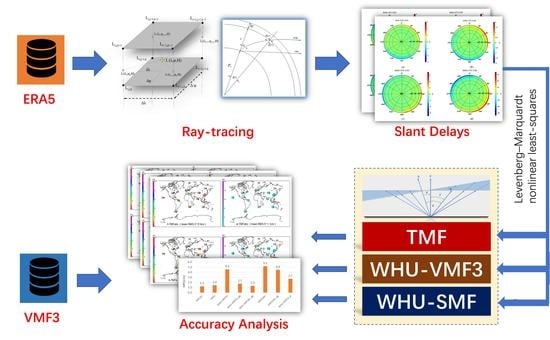
2. Materials and Method

The flow chart of the study procedure is presented in Figure 1. Firstly, ERA5 data for several IGS stations containing the pressure, temperature, and humidity fields, were retrieved from the ECMWF. Then, ray-tracing was performed at various elevation and azimuth angles for each IGS station. Finally, the TMF was fitted using mapping factors calculated by ray-traced slant delays and zenith delays.

2.1. Ray-Tracing

2.1.1. Refractivity

The refractivity of the troposphere, N, is defined by:

$$N={10}^6\times \left(n-1\right)$$

(1)

where n is the refractive index, which represents the ratio of the propagating speed of radio waves in a vacuum and in the troposphere, respectively. Smith and Weintraub [62] gave the relationship below:

$$N=k_1\frac{P_d}{T}{Z}_d^{-1}+\left(k_2^{}\frac{P_w}{T}+k_3\frac{P_w}{T^2}\right)Z_w^{-1}$$

(2)

where $P_d$ is the partial pressure of dry gases (in hPa); $P_w$ is the water vapor pressure (in hPa); T is the temperature (in degree Kelvin); $Z_d^{}$ is the compressibility factor for dry air; $Z_w^{}$ is the water vapor compressibility factor; and $k_i$ (i = 1, 2, 3) are refractivity constants, of which different versions are suggested by various authors [63]. In this study, we set constants in accordance with most ray-tracing software [64], which are $k_1=77.689$K/hPa, $k_2=71.2952$K/hPa and $k_3=\mathrm{375,463}$K²/hPa [9,65].

The water vapor pressure can be calculated using the following equation [66]:

$$P_w=\frac{q}{\left(\epsilon +\left(1-\epsilon \right)q\right)}P\approx \frac{q}{\left(0.622+0.378q\right)}P$$

(3)

where $\epsilon$ is the ratio of the molar masses of water vapor and dry gases, $q$ is the specific humidity, and $P$ is the total pressure.

Assuming that air in the troposphere behaves as an ideal gas, Equation (2) becomes [4,64]:

$$\begin{array}{l}N=N_h+N_w\\ N_h=k_1\frac{P}{T}{Z}_d^{-1}\\ N_w=({k^{\prime }}_2^{}\frac{P_W}{T}+k_3\frac{P_W}{T^2})Z_w^{-1}\end{array}$$

(4)

where $k_2^{\prime }=k_2-k_1\frac{p_w}{T}{Z}_d^{-1}$; $N_h$ and $N_w$ are denominated as the hydrostatic and wet components of the refractivity, respectively [5].

2.1.2. Tropospheric Delay

The tropospheric delay can be defined as the discrepancy between the propagation time of a GNSS signal in the troposphere and in a vacuum:

$$\begin{array}{l}STD=SHD+SWD\\ ={\displaystyle \underset{ray}{\overset{}{\int }}nds}-{\displaystyle \underset{vac}{\overset{}{\int }}1ds}={\displaystyle \underset{ray}{\overset{}{\int }}nds}-{\displaystyle \underset{ray}{\overset{}{\int }}1ds}+{\displaystyle \underset{ray}{\overset{}{\int }}1ds}-{\displaystyle \underset{vac}{\overset{}{\int }}1ds}\\ ={\displaystyle \underset{ray}{\overset{}{\int }}(n-1)ds}+\left[{\displaystyle \underset{ray}{\overset{}{\int }}1ds}-{\displaystyle \underset{vac}{\overset{}{\int }}1ds}\right]={10}^{-6}{\displaystyle \underset{ray}{\overset{}{\int }}Nds}+\tau \end{array}$$

(5)

where $STD$, $SHD$ and $SWD$ denote the slant total delay, slant hydrostatic delay, and slant wet delay, respectively; $\tau$ is the geometric delay.

Inserting Equation (4) into Equation (5), we find:

$$\begin{array}{l}SHD={10}^{-6}{\displaystyle \underset{ray}{\overset{}{\int }}{N}_{h}ds}+\tau ={10}^{-6}{k}_1{\displaystyle \underset{ray}{\overset{}{\int }}\frac{P}{T}{Z}_d^{-1}ds+\tau }\\ SWD={10}^{-6}{\displaystyle \underset{ray}{\overset{}{\int }}{N}_{\mathrm{w}}ds}={10}^{-6}{\displaystyle \underset{ray}{\overset{}{\int }}({k^{\prime }}_2\frac{P_W}{T}+k_3\frac{P_W}{T^2})Z_w^{-1}ds}\end{array}$$

(6)

The meteorological parameters in Equation (6) can be obtained from radiosonde data [60,67,68], empirical models (e.g., UNB3m [13], GPT2w [15], ITG [19], and GPT3 [40]) or a Numerical Weather Model (NWM, e.g., ERA-Interim [69], MANAL [70], and ERA5 [61]). Since radiosonde data is rather sparse in time and location, of which profile has to be extrapolated to upper levels [71] by using profiles of a standard atmosphere (e.g., USSA66 [10], CIRA86 [72], and NRLMSISE-00 [12]), and the accuracy of empirical meteorological models are limited [9], modern researchers are inclined to use NWM with high spatial-temporal resolution.

2.1.3. ERA5 and Appropriate Land Cover Radius

The ERA5 reanalysis data produced by the ECMWF was used in this study. As the fifth generation of ECMWF atmospheric reanalysis of the global climate, ERA5 covers the period from 1979 to the present. It provides hourly estimates of atmospheric variables such as air pressure $P$, temperature $T$, specific humidity $q$, and geopotential $\Phi$, at a horizontal resolution of 0.25° (~31 km), on 137 model levels from the surface up to 0.01 hPa (~80 km). We downloaded some regional ERA5 data containing daily parameters $\left\{P,T,q,\Phi \right\}$ (in the format of grib) and found the size of a unit grid (0.25° × 0.25°) is ~15.5 Kb. There are 1,036,800 unit grids for a global file, and the file size can reach up to ~15.5 Gb, which will lead to too significant a computational burden. Hence, it is necessary to find the appropriate longitude and latitude cover area of the ray-tracing for a specific station.

In Figure 2, according to the law of sines, we get:

$$\frac{R}{\sin \left(90°-(\theta +\Delta \phi )\right)}=\frac{R+H_{\max }}{\sin \left(90°+\theta \right)}$$

(7)

where $R=M$, $M$ is the meridian radius of curvature, $H_{\max }$ is the height of the neutral atmosphere top; $\theta$ is the cutoff angle.

Therefore $\Delta \phi$ can be calculated by:

$$\Delta \phi =\left(\arccos \left(\frac{R}{R+H_{\max }}\cdot \cos \theta \right)-\theta \right)$$

(8)

and $\Delta \lambda$ can be calculated by:

$$\Delta \lambda =\frac{\Delta \phi \cdot R}{r}=\{\begin{array}{c}\frac{\Delta \phi \cdot M}{N\cos \phi },\left(\left|\phi \right|\le 88°\right)\\ 180°,\left(\left|\phi \right|>88°\right)\end{array}$$

(9)

where $r=N\cdot \cos \phi$ is the radius of the parallel circle, $N$ is the radius of curvature in prime vertical.

The data set chosen for our study is comprised of data from 12 IGS (International GNSS Service) stations distributed worldwide (see Figure 3).

2.1.4. Eikonal Equation and 3D Ray-Tracing

With Maxwell’s equations and considering a medium free of currents and charges, and a short vacuum wavelength, the Eikonal equation can be written as [70]:

$${\displaystyle \sum _{\mathrm{i}=1}^3{(\frac{\partial S(\overrightarrow{x})}{\partial x_i})}^2}=n^2(\overrightarrow{x})$$

(10)

where $S$ is the optical path length; $\overrightarrow{x}$ is a position vector; $S(\overrightarrow{x})$ is referred to as the Eikonal, which can be used to compute $\nabla S(\overrightarrow{x})$ to get the ray direction; $n$ is the refractive index of a medium at the position $\overrightarrow{x}$. For a length $L$ in a ray-based system, we can get:

$$\frac{d}{dL}\left(n(\overrightarrow{x})\frac{d\overrightarrow{x}}{dL}\right)=\nabla n(\overrightarrow{x})$$

(11)

Which can be split into two first-order differential equations as:

$$\{\begin{array}{l}\frac{d\overrightarrow{x}}{dL}=\frac{\overrightarrow{v}}{n(\overrightarrow{x})}\\ \frac{d\overrightarrow{v}}{dL}=\nabla n(\overrightarrow{x})\end{array}$$

(12)

where $\overrightarrow{v}$ denotes the tangent of the trajectory at the point $\overrightarrow{x}$.

Firstly, the meteorological parameters at the point are interpolated using the adjacent grid points (see Section 2.1.5. Interpolation of meteorological parameters), and then the refractivity (see Equation(4)) is computed. The gradient of the refractivity can be obtained by two adjacent points along the ray in a spherical coordinate system $\left(r,\lambda ,\phi \right)$ via Equation (13), and partial derivatives can be calculated analytically (detailed information can be found in Appendix B of Hobiger, et al. [70]).

$$\nabla n\left(r,\lambda ,\phi \right)=\frac{\partial n\left(r,\lambda ,\phi \right)}{\partial r}\overrightarrow{r}+\frac{1}{r}\frac{\partial n\left(r,\lambda ,\phi \right)}{\partial \phi }\overrightarrow{\phi }+\frac{1}{r\cos \phi }\frac{\partial n\left(r,\lambda ,\phi \right)}{\partial \lambda }\overrightarrow{\lambda }$$

(13)

where $r$ is the radial distance, $\lambda$ is the longitude, and $\phi$ is the latitude.

Finally, the tropospheric delay can be integrated by Equation (6). For a given outgoing elevation angle, the ray-tracing will be performed three times by adding small changes on the initial elevation angle, and a quadratic function can fit delays at the given angle.

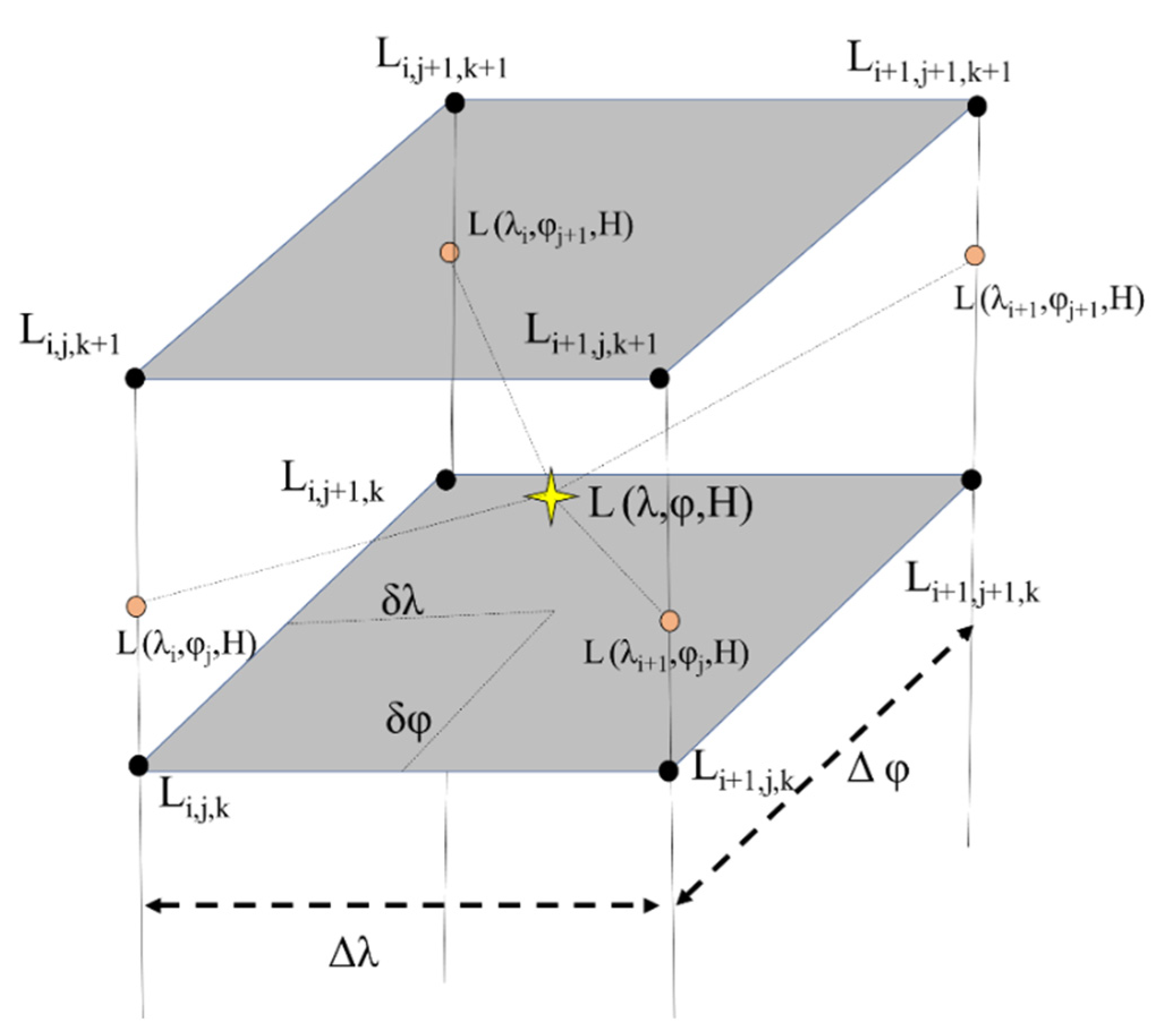
2.1.5. Interpolation of Meteorological Parameters

As shown in Figure 4, during the ray-tracing process, to obtain meteorological parameters of the point $L$ with longitude $\lambda$, latitude $\phi$ and height $H$, we may first retrieve the parameters’ values of its eight adjacent grid points from the ERA5 data. Since the heights of these grid points on the same model level are always different from each other, the interpolation can be performed vertically to the height $H$ at first and then horizontally by a bilinear method.

In the vertical direction, temperatures and humidity can be interpolated by a linear method. For the total pressure $P$ and water vapor pressure $P_W$, the following formulas are utilized in the vertical interpolation [13,16,73]:

$$P=P_0(\frac{T}{T_0}{)}^{\frac{{\mathrm{g}}_0}{R_d\beta }}$$

(14)

$$P_W=P_W{}_0{(\frac{T}{T_0})}^{\frac{g_0(\gamma +1)}{R_d\beta }}$$

(15)

where $P_0$, $T_0$, $P_W{}_0$ are meteorological values at the start point; $g_0$ is the gravity acceleration for a point at latitude $\phi$ and height $h$, the formula for the normal gravity [74] is used here; $R_d$ is the mean specific gas constant for dry air; $\gamma$ is the water vapor lapse rate parameter, and $\beta$ is the temperature lapse rate.

Since ERA5 provides data hourly, and the GNSS receiver always logs observation every 1 or 30 s, linear time interpolation between two epochs can be carried out to calculate the meteorological parameters for the time of interest.

2.1.6. Height Transformation

ERA5 is based on a geopotential height system, whereas the ray-tracing calculation is performed on the geometrical (ellipsoidal) system. Therefore, it is necessary to transform heights of the ERA5 data into geometrical height using:

$$\begin{array}{l}h=H+N\\ H=\frac{\Phi }{\overline{\gamma }(\phi ,\lambda ,H)}\end{array}$$

(16)

where $h$ is the ellipsoidal height; $H$ is the orthometric height; $N$ is the geoid undulation; $\Phi$ is the geopotential provided by ERA5; $\overline{\gamma }(\phi ,\lambda ,h)$ is the mean gravity acceleration between the geoid and the point $(\phi ,\lambda ,h)$.

2.1.7. Asymmetsry Demonstration of Slant Delays

Tropospheric slant delays were ray-traced hourly with 1° steps at elevations angles from 3° to 90° (the zenith direction), and 1° steps on azimuths from 0° to 359°. Therefore there are 734,400 (86 × 360 × 24) grid points for a site each day. To show the spatial asymmetry of the SHDs and SWDs visually, we created skyplots in various directions by removing the average value over all azimuths for each elevation. We calculated the mean value, Root Mean Square (RMS), and range (max minus min) for ray-traced SHDs and SWDs at a given elevation angle $\theta$ according to the following formulas:

$$mean\left(\theta \right)=\tilde{L}\left(\theta \right)={\displaystyle \sum _{i=1}^n{L}_i\left(\theta \right)}/n$$

(17)

$$RMS\left(\theta \right)=\sqrt{{\displaystyle \sum _{i=1}^n\Delta {\left(\theta \right)}_i{}^2}/n}$$

(18)

$$range(\theta )=\max \left(\Delta {(\theta )}_i\right)-\min \left(\Delta {(\theta )}_i\right)$$

(19)

$$\Delta {\left(\theta \right)}_i=L_i\left(\theta \right)-\tilde{L}\left(\theta \right)$$

(20)

where $L_i\left(\theta \right)$ is the slant delay at the i-th azimuth of elevation angle $\theta$, $\tilde{L}\left(\theta \right)$ represents the mean value of $L_i\left(\theta \right)$, and n is the number of azimuths.

2.2. Construction of TMF

2.2.1. Tropospheric Mapping Function

In the space geodesy, we may use the general formula to represent the tropospheric delay as follows:

$$\begin{array}{l}STD\left(\theta ,\phi \right)=SHD\left(\theta ,\phi \right)+SWD\left(\theta ,\phi \right)\\ SHD\left(\theta ,\phi \right)=ZHD\cdot {\mathrm{m}}_h(\theta ,\phi )\\ SWD\left(\theta ,\phi \right)=ZWD\cdot {\mathrm{m}}_w(\theta ,\phi )\end{array}$$

(21)

where $\theta$ and $\phi$ are the elevation and azimuth angle, respectively; $STD$, $SHD$ and $SWD$ denote the slant total delay, slant hydrostatic delay, and slant wet delay, respectively; $ZHD$ and $ZWD$ stand for the zenith hydrostatic delay and zenith wet delay respectively; ${\mathrm{m}}_h(\theta ,\phi )$ and ${\mathrm{m}}_w(\theta ,\phi )$ are the hydrostatic and wet mapping functions, respectively.

Almost all modern mapping functions, e.g., NMF [33], GMF [37], VMF1 [38] and VMF3 [40], take the continued fraction form [31] as their expressions:

$${\mathrm{m}}_i(\theta )=\frac{1+\frac{a_i}{1+\frac{b_i}{1+c_i}}}{\sin \theta +\frac{a_i}{\sin \theta +\frac{b_i}{\sin \theta +c_i}}} (i=h,w)$$

(22)

where a, b and c are coefficients.

Nowadays, VMF1 is one of the most popular mapping functions in GNSS analysis. The “b” and “c” coefficients of VMF1 are given by empirical equations, whereas the “a” coefficient is determined epoch-wise (00, 06, 12, 18 UTC) from ray-traced delays at 3° elevation. VMF3 is the upgrade version of VMF1, which gets an average “a” on eight equally spaced azimuth angles. The ray-tracing of VMF3 is performed through three different NWM types, resulting in three different versions of VMF3. ERA-Interim (EI) is only published in blocks every few months, not available in real-time; OP is made available at about 18 UTC for the previous day, and FC can be made available in real-time at about 09 UTC for the following day.

In Equation (22), mapping factors on all azimuths at a specific elevation angle are assumed to be equal. This assumption is not always valid, mainly due to the high spatial and temporal variation of the meteorological parameters, especially the water vapor. As a result, it may introduce non-negligible errors to the estimated ZWD parameters, the station height and receiver clock parameters.

Tilting the zenith direction in the mapping function by an angle is one possibility to represent a tropospheric gradient [32]. The representation given by Chen, et al. [44], which has been used by many scientific GNSS software such as GAMIT [26], and Bernese [25], can be written as:

$$STD\left(\theta ,\phi \right)=SHD\left(\theta \right)+SWD\left(\theta \right)+m{f}_g\left[G_{NS}\cdot \cos \phi +G_{EW}\cdot \sin \phi \right]$$

(23)

where $G_{NS}$ and $G_{EW}$ are North-South and East-West components of the tropospheric gradient parameters, respectively, and $m{f}_g=\frac{1}{\sin \theta \cdot \tan \theta +{\mathrm{C}}_i}$ is the gradient mapping function, $C_h=0.0031$ for the hydrostatic [44], $C_{\mathrm{w}}=0.0007$ for the wet [44], and $C_t=0.0032$ for the total [32] gradient mapping function.

With Equation (23), gradients can be estimated. The gradients can be split into a hydrostatic and a wet part, which are the integration of the North and East directional derivatives of the “hydrostatic” and “wet” parts of the refractivity along with the altitude [30]. One should note that it is difficult to separate the hydrostatic and wet gradients in the GNSS analysis [75] due to the similarity of the two gradient mapping functions (see Figure 5).

However, since the spatial distribution of the hydrostatic delays and the wet delays are always different, it is reasonable to estimate gradient parameters respectively for the two delays, which could be performed based on ray-traced delays from NWM.

2.2.2. The Definition of TMF

The refractivity at sea level inevitably increases from the warmer regions toward the colder regions. In the lower troposphere, the surfaces of constant refractivity acquire a general slope [59]. One method that can be used to model azimuthal asymmetry is based on a “tilted” atmosphere assumption [32]. Meindl, et al. [49] gave the relations between the tropospheric and the geometric zenith direction to derive the gradient parameters’ concept. In this study, we applied this relation to the mapping functions.

As shown in Figure 6, assuming that there is a small angle $\beta$ between the tropospheric zenith direction $\tilde{Z}$ and the geometric zenith direction $z$, we get:

$$\begin{array}{cc}\tilde{z}& =z+\beta \cos \left(\phi -{\phi }_0\right)\\ & =z+\beta \cos {\phi }_0\cos \phi +\beta \sin {\phi }_0\sin \phi \end{array}$$

(24)

where $\tilde{z}$ denotes the tropospheric zenith angle; $z$ is the geometric zenith angle and $z={90}^{°}-\theta$; ${\phi }_0$ is the azimuth of $\tilde{Z}$ with respect to $z$; $\phi$ represents the azimuth of the GNSS observation.

Introducing tropospheric elevation angle $\tilde{\theta }$ as an argument for the mapping functions, and utilizing the Taylor series to approximate the slant delay linearly as:

$$\begin{array}{l}STD\left(\theta ,\phi \right)=STD\left(\tilde{\theta }\right)=STD\left(\theta -\beta \cos \left(\phi -{\phi }_0\right)\right)\\ =STD\left(\theta -\left(\beta \cos {\phi }_0\cos \phi +\beta \sin {\phi }_0\sin \phi \right)\right)\\ \doteq ZHD\cdot {\mathrm{m}}_h(\theta )+ZWD\cdot {\mathrm{m}}_w(\theta )+\left[G_{NS}\cdot \cos \phi +G_{EW}\cdot \sin \phi \right]\cdot \frac{\partial {\mathrm{m}}_f}{\partial \theta }\end{array}$$

(25)

where $\tilde{\theta }={90}^{\circ }-\tilde{z}$; $G_{NS}$ and $G_{EW}$ are the tropospheric gradient parameters; and $\frac{\partial {\mathrm{m}}_f}{\partial \theta }$ is the derivative of the arbitrary mapping function ${\mathrm{m}}_f$ with respect to the elevation angle $\theta$. Equation (23) may also be obtained from Equation (25) by using.${\mathrm{m}}_f=\frac{1}{\sin \theta }$.

Equation (25) only the first-order term of the Taylor series is kept, which may introduce the linearization error. Therefore in the mapping function expression, we reserve the $\beta$ and ${\phi }_0$ as two variables, which can be estimated together with coefficients $a_i$, $b_i$ and $c_i$, directly by mapping factors of ray-traced slant delays over zenith delay. Therefore, the Equation (22) can be rewritten as:

$${\stackrel{˄}{\mathrm{m}}}_i\left(\tilde{\theta }\right)=\frac{1+\frac{a_i}{1+\frac{b_i}{1+c_i}}}{\sin \tilde{\theta }+\frac{a_i}{\sin \tilde{\theta }+\frac{b_i}{\sin \tilde{\theta }+c_i}}},(i=h,w)$$

(26)

where $\tilde{\theta }=\{\begin{array}{c}\theta -\beta \cos \left(\phi -{\phi }_0\right),\theta <{90}^{°}\\ \theta -\beta ,\theta ={90}^{°}\end{array}$, the unique value for $\tilde{\theta }$ when $\theta ={90}^{°}$ is to avoid the multivalued problem at the geometric zenith direction, and ${\stackrel{˄}{m}}_i\left(\tilde{\theta }\right)$ are called TMF. With this new mapping function, which depends both on the elevation and azimuth angle, it would be unnecessary to estimate the gradient parameters.

2.2.3. Fitting of TMF

The mapping function can be expressed as:

$${\stackrel{˄}{m}}_i\left(\tilde{\theta }\right)=\frac{RS{D}_i\left(\theta ,\phi \right)}{RZ{D}_i}, (i=h,w)$$

(27)

where $RS{D}_i\left(\theta ,\phi \right)$ and $RZ{D}_i$ are the ray-traced slant delays ($i=h$ for SHD, and $i=w$ for SWD) and zenith delays ($i=h$ for ZHD and $i=w$ for ZWD), respectively.

According to Equation (26), the parameters to be estimated for the TMF are $\left\{\beta ,{\phi }_0,a_i,b_i,c_i\right\}$. The nonlinear fit was achieved by the Levenberg–Marquardt method.

Since the ERA5 data is very hard-disk-consuming and the ray-tracing is rather time-consuming, several computation approaches were investigated. As listed in

Table 1. Key parameters of the four fitting schemes.

Scheme	Resolution of ERA5			Number of Data for Fitting
	Horizontal	Temporal	Pressure Levels	Elevations × Azimuths
1	0.25° × 0.25°	1-hour1y	137	87 × 360
2	0.25° × 0.25°	1-hour1y	137	18 × 24
3	1° × 1°	1-hour1y	137	87 × 360
4	1° × 1°	1-hour1y	137	18 × 24

, ray-traced slant delays based on two versions of ERA5 production (with a spatial resolution of 0.25° × 0.25° and 1° × 1°), were used to fit mapping functions by two outgoing elevation and azimuth angles selection strategies: using all 87 outgoing elevations and 360 azimuths, or 18 outgoing elevation angles (3°, 4°, 5°, 6°, 7°, 8°, 9°, 10°, 12°, 15°, 20°, 25°, 30°, 36°, 42°, 50°, 63°, 80°), which were picked in such a way as to cover the whole elevation range [34], and 24 azimuths (15° steps from 0° to 345°). It should be noted that the ray-traced zenith delay $RZ{D}_i$ was computed at the geometric zenith direction, not the tropospheric zenith direction. It would be rigorous to perform ray-tracing again at the fitted tropospheric zenith direction, computing the factor between the geometric zenith delay and the tropospheric zenith delay, and multiply it by the initial TMF. However, since the $\beta$ is very small (with an observed mean value of 31″ found by Meindl, et al. [49] and 25″ in our experiments), the difference between the two delays is negligible.

The mapping functions’ coefficients were determined through a nonlinear least square adjustment over all selected elevation and azimuth angles. After that, mapping factors outputted from these fitted mapping functions were multiplied by the ray-traced zenith delay (ZHD or ZWD) to get the TMF-derived slant delays (SHD or SWD). Ray-traced slant delays by the first scheme (ERA5 with a horizontal resolution of 0.25° × 0.25°, at all 86 elevations and 360 azimuths) were used as truth values.

After the appropriate scheme was determined, a series of mapping functions that are based on the TMF, and the VMF3 concept, without or with gradient estimation, were designed and tested. As listed in

Table 2. A list of approaches for mapping functions and gradients used in this study.

Code	Elevations	Azimuths	Determination of		Estimation of Gradient
			a	b, c
TMFabc	18	8	LS	LS	no
TMFa	18	8	LS	VMF3 ①	no
WHU-VMF3a ②	1	8	mean	VMF3 ①	no
WHU-VMF3a_g ②	1 (18) ③	8	mean	VMF3 ①	total
WHU-VMF3a_gg ②	1 (18) ③	8	mean	VMF3 ①	h,w ④
WHU-SMFabc_gg ②	18	8	LS	LS	h,w ④
VMF3abc	1	8 [40]	VMF3 ①	VMF3 ①	no
VMF3abc_gg	1	16 [46]	VMF3 ①	VMF3 ①	VMF3 ①

①: VMF3_EI: site-wise version (Available from https://vmf.geo.tuwien.ac.at/trop_products/GNSS/, accessed on 15 March 2021) ②: Using the same ray-traced delays as TMF, calculated by WHURT. ③: One elevation angle (3°) for coefficient “a” and 18 elevation angles (3°, 4°, 5°, 6°, 7°, 8°, 9°, 10°, 12°, 15°, 20°, 25°, 30°, 36°, 42°, 50°, 63°, 80°) for gradients estimation. ④: The gradients were estimated both for the hydrostatic and wet parts.

, “WHU-” denotes that the ray-traced delays of WHURT serve as the basis for the calculation of mapping function coefficients, using the same model as VMF3 (see Equation (22)); LS means Least-Squares; eight equally spaced azimuth angles (0°:45°:345°) were chosen to be consistent with VMF3 [40]; VMF3 in the last three column means the value of the coefficient or gradients were retrieved from the VMF3_EI site-wise version.

2.3. Performance Test of TMF

In order to assess the errors of mapping functions effectively, their function values at some selected elevations and azimuths were multiplied by the ray-traced zenith delay to get the nominal slant delays; namely, the MF (mapping function)-derived slant delays. Then the RMS of differences between the ray-traced slant delays and the MF-derived slant delays were calculated by:

$$RMS=\sqrt{{\displaystyle \sum _{i=1}^m{\displaystyle \sum _{j=1}^n{\left(S{D}_{ij}^{ray}-S{D}_{ij}^{\mathrm{MF}}\right)}^2}}/\left(n\cdot m\right)}$$

(28)

where $m$ = 86, $n$ = 24 are the number of elevation angles and azimuths, respectively; $S{D}_{ij}^{ray}$ is the ray-traced SHD or SWD, and $S{D}_{ij}^{\mathrm{MF}}$ is the MF-derived SHD or SWD.

The improvement percentage of a mapping function against another mapping function was computed as:

$$IPV=\frac{RM{S}_{MF\mathrm{i}}-RM{S}_{MFj}}{RM{S}_{MFi}}\times 100$$

(29)

According to the rule of thumb [34,36], one-third of the mapping function delay error at the lowest elevation angle included in the analysis can be seen as station height error, which indicates the impact of the mapping functions on the position domain without processing GNSS observations.

3. Results

3.1. Tropospheric Delay Asymmetry

The tropospheric delays’ asymmetry can be assessed visually by skyplots with the removal of the average value over all azimuths on each elevation angle. Due to space limitation, only a few of them are present here exemplarily to demonstrate the spatio-temporal variability. Figure 7 and Figure 8 are the IGS station SHAO results on 21 July and 26 December 2018, respectively. The epoch of the left and right panel is 0:00 UTC and 5:00 UTC, respectively.

Figure 7d shows much more significant anisotropy (please note the disparity in the bounds of the colour bars) than Figure 7c, which means that there was a quick variation of SWD from 0:00 to 5:00 UTC. This may be due to the fast-changing distribution of humidity, the typical summer weather conditions at Shanghai, where the SHAO station is located.

The situation is a little different on 26 December. As shown in Figure 8, although the elevation-dependent pattern is similar to Figure 7, SHD shows more spatial variability than SWD this time. The SHD range can reach up to ~10 cm at 5° elevation, while the SWD range is no more than several centimeters. This result may be caused by the fact that there is much less water vapor in winter than in summer in Shanghai. However, a comparison between Figure 8c,d shows that the temporal variations of SWD are still more complicated than SHD.

In order to get a more quantitative investigation on the results at low elevations, we summarise the statistical result of slant delays at four specific elevations: 5°, 10°, 15° and 20° in

Table 3. Representative ray-tracing slant delays for SHAO located in Shanghai on 21 July 2018.

UTC	Elevation Angle	SHD (m)			SWD (m)
		Mean	Range	RMS	Mean	Range	RMS
0:00	5°	23.135	0.040	0.012	3.515	0.119	0.037
	10°	12.706	0.015	0.004	1.850	0.029	0.007
	15°	8.703	0.007	0.002	1.255	0.018	0.004
	20°	6.636	0.004	0.001	0.953	0.012	0.003
5:00	5°	23.102	0.039	0.011	3.894	0.678	0.245
	10°	12.689	0.015	0.004	2.078	0.245	0.080
	15°	8.691	0.007	0.002	1.410	0.118	0.037
	20°	6.627	0.004	0.001	1.071	0.066	0.021

and

Table 4. Representative ray-tracing slant delays for SHAO located in Shanghai on 26 December 2018.

UTC	Elevation Angle	SHD (m)			SWD (m)
		Mean	Range	RMS	Mean	Range	RMS
	5°	23.525	0.100	0.034	1.632	0.075	0.026
0:00	10°	12.896	0.035	0.012	0.858	0.024	0.008
	15°	8.828	0.017	0.006	0.581	0.012	0.004
	20°	6.730	0.010	0.003	0.440	0.007	0.002
	5°	23.492	0.100	0.035	1.540	0.022	0.007
5:00	10°	12.876	0.036	0.012	0.806	0.005	0.001
	15°	8.814	0.019	0.006	0.545	0.003	0.001
	20°	6.719	0.011	0.003	0.414	0.002	0.000

. There is much in common between the two tables. Firstly, the SHD and SWD and their range and RMS all tend to increase positively as elevation angle decreases. However, the SHD is always 6–15 times as large as the SWD. Secondly, the RMS of SHD and SWD at an elevation above 15° are mainly at the level of several millimetres. Furthermore, the RMS and range at the 5° elevation are always ten times as lager as that at the 20° elevation, both for SHD and SWD. Results above indicate that both the SHD and the SWD may present decametric asymmetry at low elevations.

3.2. TMF Fitting

The results of the four fitting schemes introduced in Table 1 are listed in

Table 5. Statistic result of TMF-derived slant delays, which are the product of the TMF and the ray-traced zenith delays. The meaning of the postfix numbers is listed in Table 2.

Elevation Angle	ΔSHD (cm)
	bias1	RMS1	bias2	RMS2	bias3	RMS3	bias4	RMS4
3°–15°	0.0	0.3	0.0	0.3	−0.3	0.7	−0.3	0.7
15°–89°	0.0	0.0	0.0	0.1	−0.2	0.3	−0.2	0.3
Elevation Angle	ΔSWD (cm)
	bias1	RMS1	bias2	RMS2	bias3	RMS3	bias4	RMS4
3°–15°	0.0	1.9	0.0	2.0	0.0	8.0	0.0	7.9
15°–89°	0.0	0.3	0.1	0.4	0.4	2.8	0.3	2.8

, in which elevations are divided into two bands: low elevation $\left(3°\le \theta \le 15°\right)$ and high elevation $\left(15°<\theta <90°\right)$. As shown in Table 5, there is no apparent difference for bias and RMS between the two elevation and azimuth angle selection strategies (1 vs. 2, or 3 vs. 4). However, the horizontal resolution of ERA5 has a significant impact on the results. The RMS of the fitted SWDs based on ERA5 with 1° × 1° horizontal resolution is four and 7~9 times larger than that of the 0.25° × 0.25°, at low and high elevation angle bands, respectively. Results for SHD are similar but a little better. Hence, we use Scheme 2 in Table 1 (ERA5 with a horizontal resolution of 0.25° × 0.25°, at 18 selected elevations and 24 azimuths) to implement ray-tracing in the following research, which aims to keep a balance between the computational accuracy and the efficiency.

3.3. TMF Performance

The MF-derived slant delays are the production of the mapping factors and the ray-traced zenith delay. The discrepancy compared with the ray-traced slant delays can directly reflect the accuracy of a mapping function.

Figure 9 shows the RMS scatters of the discrepancies between MF-derived and ray-traced delays at the 5° elevation angle for the 12 globally distributed IGS stations listed in Table 1, at 96 epochs on four days (doy: 74, 202, 246, and 360) in 2018. Since each station’s computation is independent of each other, such a graph would be an excellent way to reflect the global applicability of a mapping function. As shown in Figure 9, the TMFabc performs the best globally, with RMS of almost the same level for each station. Notably, the station FAIR and YAKT have the highest accuracy of wet delays. This may be due to the cold and dry weather on high latitudes in the northern hemisphere.

In contrast, there are much more variations with the symmetric mapping functions based on the VMF3 concept (WHU-VMF3a, WHU-VMF3a_gg, and WHU-VMF3a_g), especially for the wet delays. However, comparing WHU-VMF3a_gg with WHU-VMF3a shows that the estimation of gradients improves the result dramatically, although not as good as that of TMFs.

The performances of the original VMF3 (VMF3abc and VMF3abc_gg) are the worst but not surprising since the resolution of the NWM used by us (0.25° × 0.25°, 137 model levels, 1 h) is superior to that of VMF3 (1° × 1°, 25 pressure levels, 6 h [40]). VMF3abc_gg improves accuracy mainly on hydrostatic delays but very slightly on wet delays. We can conclude that the resolution of the NWM limits the accuracy of VMF3-derived wet gradients.

Table 6. Accuracy of MF-derived hydrostatic delays.

Code	BIAS (cm)	RMS (cm)	BIAS at 5° (cm)	RMS at 5° (cm)
TMFabc	0.0	0.2	0.0	0.5
TMFa	0.0	0.2	−0.1	0.6
WHU-VMF3a	0.0	0.6	−0.2	2.0
WHU-VMF3a_gg	0.0	0.2	−0.2	0.7
WHU-SMFabc_gg	0.0	0.2	0.1	0.5
VMF3abc	−0.1	0.8	−0.9	2.4
VMF3abc_gg	−0.1	0.5	−0.9	1.5

and

Table 7. Accuracy of MF-derived wet delays.

Code	BIAS (cm)	RMS (cm)	BIAS at 5° (cm)	RMS at 5° (cm)
TMFabc	0.0	0.5	0.0	1.1
TMFa	0.0	0.5	−0.1	1.3
WHU-VMF3a	0.0	1.3	−0.3	4.1
WHU-VMF3a_gg	0.0	0.6	−0.3	1.6
WHU-SMFabc_gg	0.0	0.5	−0.1	1.2
VMF3abc	0.0	1.5	0.1	4.5
VMF3abc_gg	0.0	1.4	0.1	4.2

give the statistics results of the hydrostatic and wet part of all mapping functions (except for the WHU-VMF3a_g, of which the hydrostatic and wet delays cannot be separated), respectively. These two tables clearly show that the differences between various models are primarily in the RMS; the differences concerning the bias are minimal.

As shown in Table 6, TMFabc performs the best among all hydrostatic mapping functions, with the minimal RMS_all (RMS for all elevation angles) and the minimal RMS_5° (RMS for the 5° elevation angle). Compared with WHU-VMF3a, TMFabc improves the RMS_all and the RMS_5° by 68% and 74%, respectively. By the extra estimation of hydrostatic gradients, WHU-VMF3a_gg improves these by 62% and 65%, respectively. The accuracy of WHU-SMFabc_gg is only slightly lower than TMFabc. For VMF3, with gradients, the RMS_all and the RMS_5° can be improved by 35% and 39%, respectively. However, it seems that there are some slight systematic errors between the VMF3-derived and the WHURT-derived hydrostatic slant delays, which would be mainly due to the difference in the NWMs. By adopting the b and c coefficients of VMF3, TMFa can achieve higher accuracy than WHU-VMF3a_gg, with less computational cost than TMFabc, which could be meaningful for large-scale computing.

In Table 7, all MF-derived wet delays’ biases are closer to zero than the hydrostatic ones, but mostly with larger RMSs. TMFabc is still the most accurate, followed by the WHU-SMFabc_gg and TMFa. There is no significant difference between TMFabc and WHU-SMFabc_gg for most stations at most epochs, except for some particular conditions. Figure 10 shows this exemplarily for IGS station SHAO on the doy 202, 2018, when typhoon “Ampil” passed Shanghai. During 3:00–5:00 and 18:00–20:00 UTC, there are apparent improvements for TMFabc against WHU-SMF3abc_gg. WHU-VMF3a_gg improves the RMS_all and the RMS_5° of WHU-VMF3a by 59% and 62%, respectively.

Figure 11 shows the RMS scatters of all kinds of MF-derived total delays at the 5° elevation angle, which are calculated by $rm{s}_{total}=\sqrt{rm{s}_h^2+rm{s}_w^2}$, where $rm{s}_h^{}$, and $rm{s}_w^{}$ are the RMS_5° of the hydrostatic and wet MF-derived delays respectively. TMFabc performs the best. The improvement percentage of TMFabc against WHU-VMF3a, WHU-VMF3a_g, and WHU-VMF3a_gg can reach up to 73%, 54%, and 29%, respectively. Even by directly adopting the two coefficients b and c of VMF3 instead of estimating them, TMFa can still improve WHU-VMF3a, WHU-VMF3a_g WHU-VMF3a_gg by 68%, 47%, and 18%, respectively. It is worth noting that the improvement percentage of WHU-VMF3a_gg against WHU-VMF3a_g is 35%, which indicates that a separate estimation of the hydrostatic and wet gradients is preferable to a coarse estimation of the total gradients. Compared with WHU-VMF3a, the reduced RMS_5° ratio between WHU-VMF3a_gg and TMFabc is 2.8/3.3, which is close to the value found by Landskron, et al. [46] that two-thirds of the azimuthal asymmetry can be described by the first-order gradients based on the VMF3 mapping function.

4. Discussion

Investigation of 360-degree ray-traced delays based on NWM revealed that both the SHD and SWD show azimuthal asymmetry, reaching up to decimeter level at low elevation angles below 15°. When a symmetric mapping function is used, the accuracy would not be as bad as expected, since the cutoff elevation angle is always set to 10° or 15° for most geodetic applications, which are typically based on double-differenced solutions. However, significant correlations between troposphere zenith delay parameters, station height, and receiver clock parameters are found [48]. The situation may be considerably improved by lowering the elevation cutoff angle. According to the rule of thumb, the delay path error at a 5° elevation will map to the station height at a ratio of 1/3 [34,36]. Therefore, it is essential to model variations of the slant delays on the elevation and the azimuth.

The gradient parameters have been used as a supplement for a symmetric mapping function to model the azimuthal asymmetry for decades. However, in former GNSS studies [43,44,45,51], only the total gradients can be estimated, due to the difficulty of distinguishing the hydrostatic and wet gradient mapping functions. The WHU-VMF3a_g can be deemed a simulation for such tropospheric delay strategy, of which accuracy is not as good as that of separate estimation of hydrostatic and wet gradients (WHU-VMF3a_gg). In contrast, TMF can achieve better accuracy than a VMF3-like symmetric mapping function enhanced by estimation of respective gradients, of which coefficients b and c are not estimated but obtained from climatology data, and a is determined at a single elevation angle. The result of SMFabc_gg indicates that: (1) If a symmetric mapping function is not accurate enough, it would be difficult to precisely model the anisotropy part of the tropospheric delays by gradients. Therefore, estimating coefficients by least-squares on sufficient widespread elevation angles is necessary. (2) Assuming a proper mapping function is applied, gradients can describe the bulk of the tilting troposphere in most situations. However, there could still be some non-negligible high-order residuals [46], especially under some particular conditions such as severe weather scenarios [76].

The assumption of a tilted troposphere can explain most of the actual distribution of the Earth’s troposphere. However, the tropospheric delay error of TMF is about ±1.2 cm at the 5° elevation angle, corresponding to a station height error of ±4 mm. A tilted troposphere may not fully explain the variability of the tropospheric delays, which is also affected by other factors, such as the highly variable water vapor. Therefore, further study should be investigated on how to model the residual delays more precisely based on TMF, if higher accuracy is required. Besides, various NWMs featuring high spatio-temporal resolution produced by different agencies could be utilized together to validate each other and achieve a more robust mapping function.

5. Conclusions

In this research, ERA5 data retrieved from ECMWF with the highest spatial-temporal resolution was applied to compute the tropospheric slant delays by the ray-tracing method. It is found that azimuthal variation of tropospheric delay at low elevation angles can reach up to several decimeters. Traditional three order continued fraction mapping functions have been developed based on the assumption of atmospheric spherical symmetry, in which the azimuthal variation of tropospheric delays is neglected. To overcome shortcomings caused by such mapping functions, TMF is built by tilting the zenith direction of the mapping function, of which coefficients were fitted by Levenberg–Marquardt nonlinear least square method. We found that the horizontal resolution of NWM has a significant impact on mapping functions. However, it is not necessary to choose all elevations and azimuths. Fitting at 18 selected elevations and 24 azimuths are proved to be enough to produce comparable results with complete sampling.

The performances of several mapping functions based on the TMF and VMF3 concept were assessed quantitatively by using the ray-traced slant delays as reference values. Results show that TMF can improve 54% against the VMF3-like symmetric mapping function enhanced by estimating total gradients (WHU-VMF3a_g). According to the rule of thumb, a similar improvement in height parameter estimation is expected in GNSS analysis, which needs to be verified in our further study. A global grid-wise TMF can be developed for an arbitrary station’s interpolation. To balance the accuracy and the computational cost, TMFa may be a good choice. Moreover, it would be necessary for the real-time application to derive TMF based on high-quality operational or forecast versions of NWM, including in-situ meteorological observations if possible.

References

1. Yang, F.; Guo, J.; Meng, X.; Shi, J.; Xu, Y.; Zhang, D. Determination of Weighted Mean Temperature (Tm) Lapse Rate and Assessment of Its Impact on Tm Calculation. IEEE Access 2019, 7, 155028–155037. [Google Scholar] [CrossRef]
2. Zhang, D. The Study of the GNSS Tropospheric Zenith Delay Model and Mapping Function. Ph.D. Thesis, Wuhan University, Wuhan, China, 2017. [Google Scholar]
3. Hopfield, H. Two-quartic tropospheric refractivity profile for correcting satellite data. J. Geophys. Res. 1969, 74, 4487–4499. [Google Scholar] [CrossRef]
4. Saastamoinen, J. Atmospheric correction for the troposphere and stratosphere in radio ranging satellites. Geophys. Monogr. Ser. 1972, 15, 247–251. [Google Scholar]
5. Davis, J.; Herring, T.; Shapiro, I.; Rogers, A.; Elgered, G. Geodesy by radio interferometry: Effects of atmospheric modeling errors on estimates of baseline length. Radio Sci. 1985, 20, 1593–1607. [Google Scholar] [CrossRef]
6. Berrada Baby, H.; Gole, P.; Lavergnat, J. A model for the tropospheric excess path length of radio waves from surface meteorological measurements. Radio Sci. 1988, 23, 1023–1038. [Google Scholar] [CrossRef]
7. Ifadis, I.I. The Atmospheric Delay of Radio Waves: Modeling the Elevation Dependence on a Global Scale; Technical Report 38L; Chalmers University of Technology: GÄoteborg, Sweden, 1986. [Google Scholar]
8. Askne, J.; Nordius, H. Estimation of tropospheric delay for microwaves from surface weather data. Radio Sci. 1987, 22, 379–386. [Google Scholar] [CrossRef]
9. Zhang, D.; Guo, J.; Chen, M.; Shi, J.; Zhou, L. Quantitative assessment of meteorological and tropospheric Zenith Hydrostatic Delay models. Adv. Space Res. 2016, 58, 1033–1043. [Google Scholar] [CrossRef]
10. COESA. U.S. Standard Atmosphere Supplements, 1966; U.S. Government Printing Office: Washington, DC, USA, 1966; pp. 101–102.
11. Kirchengast, G.; Hafner, J.; Poetzi, W. The CIRA86aQ_UoG Model: An Extension of the CIRA-86 Monthly Tables Including Humidity Tables and a Fortran95 Global Moist Air Climatology Model; Institute for Meteorology and Geophysics, University of Graz: Graz, Austria, 1999; p. 18. [Google Scholar]
12. Picone, J.; Hedin, A.; Drob, D.P.; Aikin, A. NRLMSISE-00 empirical model of the atmosphere: Statistical comparisons and scientific issues. JGR Space Phys. (1978–2012) 2002, 107, SIA 15-1–SIA 15-16. [Google Scholar] [CrossRef]
13. Leandro, R.; Santos, M.; Langley, R.B. UNB neutral atmosphere models: Development and performance. In Proceedings of the ION NTM, Monterey, CA, USA, 18–20 January 2006. [Google Scholar]
14. Morris, A. Standard Temperature and Pressure. Ind. Heat. 2012, 80, 22. [Google Scholar]
15. Böhm, J.; Möller, G.; Schindelegger, M.; Pain, G.; Weber, R. Development of an improved empirical model for slant delays in the troposphere (GPT2w). GPS Solut. 2015, 19, 433–441. [Google Scholar] [CrossRef] [Green Version]
16. Leandro, R.F.; Santos, M.C.; Langley, R.B. A North America wide area neutral atmosphere model for GNSS applications. Navigation 2009, 56, 57. [Google Scholar] [CrossRef]
17. RTCA. Minimum Operational Performance Standards for Global Positioning System/Wide Area Augmentation System Airborne Equipment; DO-229D; RTCA, Inc.: Washington, DC, USA, 13 December 2006; p. 564. [Google Scholar]
18. Schüler, T. The TropGrid2 standard tropospheric correction model. GPS Solut. 2014, 18, 123–131. [Google Scholar] [CrossRef]
19. Yao, Y.; Xu, C.; Shi, J.; Cao, N.; Zhang, B.; Yang, J. ITG: A New Global GNSS Tropospheric Correction Model. Sci. Rep. 2015, 5, 10273. [Google Scholar] [CrossRef] [Green Version]
20. Li, W.; Yuan, Y.; Ou, J.; Chai, Y.; Li, Z.; Liou, Y.-A.; Wang, N. New versions of the BDS/GNSS zenith tropospheric delay model IGGtrop. J. Geod. 2015, 89, 73–80. [Google Scholar] [CrossRef]
21. Chen, J.P.; Wang, J.G.; Wang, A.H.; Ding, J.S.; Zhang, Y.Z. SHAtropE-A Regional Gridded ZTD Model for China and the Surrounding Areas. Remote Sens. 2020, 12, 165. [Google Scholar] [CrossRef] [Green Version]
22. Tralli, D.M.; Lichten, S.M. Stochastic estimation of tropospheric path delays in global positioning system geodetic measurements. Bull. Géodésique 1990, 64, 127–159. [Google Scholar] [CrossRef]
23. Webb, S.R. Kinematic GNSS Tropospheric Estimation and Mitigation over a Range of Altitudes. Ph.D. Thesis, Newcastle University, Newcastle, UK, 2015. [Google Scholar]
24. Mousa, A.E.L.K.; Aboualy, N.; Sharaf, M.; Zahra, H.; Darrag, M. Tropospheric wet delay estimation using GNSS: Case study of a permanent network in Egypt. NRIAG J. Astron. Geophys. 2016, 5, 76–86. [Google Scholar] [CrossRef] [Green Version]
25. Dach, R.; Lutz, S.; Walser, P.; Fridez, P. Bernese GNSS Software Version 5.2; University of Bern: Bern, Switzerland, 2015; p. 854. [Google Scholar]
26. Herring, T.A.; King, R.W.; Floyd, M.A.; McClusky, S.C. GAMIT Reference Manual Release 10.7; Massachusetts Institute of Technology: Cambridge, MA, USA, 2018; p. 168. [Google Scholar]
27. Zhao, Q.; Yao, Y.; Yao, W.; Zhang, S. GNSS-derived PWV and comparison with radiosonde and ECMWF ERA-Interim data over mainland China. J. Atmos. Sol. Terr. Phys. 2018, 182, 85–92. [Google Scholar] [CrossRef]
28. He, Q.; Zhang, K.; Wu, S.; Shen, Z.; Wan, M.; Li, L. Precipitable Water Vapor Converted From GNSS-ZTD and ERA5 Datasets for the Monitoring of Tropical Cyclones. IEEE Access 2020, 8, 87275–87290. [Google Scholar] [CrossRef]
29. Yang, F.; Guo, J.; Meng, X.; Shi, J.; Zhang, D.; Zhao, Y. An improved weighted mean temperature (T-m) model based on GPT2w with T-m lapse rate. GPS Solut. 2020, 24. [Google Scholar] [CrossRef]
30. Barriot, J.-P.; Peng, F. Beyond Mapping Functions and Gradients; IntechOpen: London, UK, 2021. [Google Scholar] [CrossRef]
31. Marini, J.W. Correction of Satellite Tracking Data for an Arbitrary Tropospheric Profile. Radio Sci. 1972, 7, 223–231. [Google Scholar] [CrossRef]
32. Herring, T.A. Modeling Atmospheric Delays in the Analysis of Space Geodetic Data. In Refraction of Transatmospheric Signals in Geodesy; De Munck, J.C., Spoelstra, T.A., Eds.; The Netherlands Commission on Geodesy: Delft, The Netherlands, 1992. [Google Scholar]
33. Niell, A.E. Global mapping functions for the atmosphere delay at radio wavelengths. J. Geophys. Res. [Solid Earth] 1996, 101, 3227–3246. [Google Scholar] [CrossRef]
34. Niell, A.E. Preliminary evaluation of atmospheric mapping functions based on numerical weather models. Phys. Chem. Earth Part A 2001, 26, 475–480. [Google Scholar] [CrossRef]
35. Guo, J.; Langley, R.B. A New Tropospheric Propagation Delay Mapping Function for Elevation Angles Down to 2 degrees. In Proceedings of the ION GPS 2003, Portland, OR, USA, 9–12 September 2003. [Google Scholar]
36. Boehm, J.; Schuh, H. Vienna mapping functions in VLBI analyses. Geophys. Res. Lett. 2004, 31, 131–144. [Google Scholar] [CrossRef]
37. Boehm, J.; Niell, A.; Tregoning, P.; Schuh, H. Global Mapping Function (GMF): A new empirical mapping function based on numerical weather model data. Geophys. Res. Lett. 2006, 33, 4. [Google Scholar] [CrossRef] [Green Version]
38. Boehm, J.; Werl, B.; Schuh, H. Troposphere mapping functions for GPS and very long baseline interferometry from European Centre for Medium-Range Weather Forecasts operational analysis data. J. Geophys. Res. 2006, 111, B02406. [Google Scholar] [CrossRef]
39. Lagler, K.; Schindelegger, M.; Böhm, J.; Krásná, H.; Nilsson, T. GPT2: Empirical slant delay model for radio space geodetic techniques. Geophys. Res. Lett. 2013, 40, 1069–1073. [Google Scholar] [CrossRef] [Green Version]
40. Landskron, D.; Bohm, J. VMF3/GPT3: Refined discrete and empirical troposphere mapping functions. J. Geod. 2018, 92, 349–360. [Google Scholar] [CrossRef]
41. Zus, F.; Dick, G.; Dousa, J.; Wickert, J. Systematic errors of mapping functions which are based on the VMF1 concept. GPS Solut. 2015, 19, 277–286. [Google Scholar] [CrossRef]
42. Yuan, Y.B.; Holden, L.; Kealy, A.; Choy, S.; Hordyniec, P. Assessment of forecast Vienna Mapping Function 1 for real-time tropospheric delay modeling in GNSS. J. Geod. 2019, 93, 1501–1514. [Google Scholar] [CrossRef]
43. Qiu, C.; Wang, X.M.; Li, Z.S.; Zhang, S.T.; Li, H.B.; Zhang, J.L.; Yuan, H. The Performance of Different Mapping Functions and Gradient Models in the Determination of Slant Tropospheric Delay. Remote Sens. 2020, 12, 130. [Google Scholar] [CrossRef] [Green Version]
44. Chen, G.; Herring, T.A. Effects of atmospheric azimuthal asymmetry on the analysis of space geodetic data. J. Geophys. Res. Solid Earth 1997, 102, 20489–20502. [Google Scholar] [CrossRef]
45. Böhm, J.; Urquhart, L.; Steigenberger, P.; Heinkelmann, R.; Nafisi, V.; Schuh, H. A Priori Gradients in the Analysis of Space Geodetic Observations. In Reference Frames for Applications in Geosciences; Springer: Berlin/Heidelberg, Germany, 2013; pp. 105–109. [Google Scholar]
46. Landskron, D.; Bohm, J. Refined discrete and empirical horizontal gradients in VLBI analysis. J. Geod. 2018, 92, 1387–1399. [Google Scholar] [CrossRef] [PubMed] [Green Version]
47. Bar-Sever, Y.E.; Kroger, P.M.; Borjesson, J.A. Estimating horizontal gradients of tropospheric path delay with a single GPS receiver. J. Geophys. Res. 1998, 103, 5019–5035. [Google Scholar] [CrossRef] [Green Version]
48. Rothacher, M.; Springer, T.A.; Schaer, S.; Beutler, G. Processing Strategies for Regional GPS Networks; Springer: Berlin/Heidelberg, Germany, 1998; pp. 93–100. [Google Scholar]
49. Meindl, M.; Schaer, S.; Hugentobler, U.; Beutler, G. Tropospheric gradient estimation at CODE: Results from global solutions. J. Meteorol. Soc. Jpn. 2004, 82, 331–338. [Google Scholar] [CrossRef] [Green Version]
50. Lu, C.; Li, X.; Li, Z.; Heinkelmann, R.; Nilsson, T.; Dick, G.; Ge, M.; Schuh, H. GNSS tropospheric gradients with high temporal resolution and their effect on precise positioning. J. Geophys. Res. 2016, 121, 912–930. [Google Scholar] [CrossRef] [Green Version]
51. Iwabuchi, T.; Miyazaki, S.i.; Heki, K.; Naito, I.; Hatanaka, Y. An impact of estimating tropospheric delay gradients on tropospheric delay estimations in the summer using the Japanese nationwide GPS array. J. Geophys. Res. 2003, 108, 16. [Google Scholar] [CrossRef]
52. Zus, F.; Douša, J.; Kačmařík, M.; Václavovic, P.; Balidakis, K.; Dick, G.; Wickert, J. Improving GNSS Zenith Wet Delay Interpolation by Utilizing Tropospheric Gradients: Experiments with a Dense Station Network in Central Europe in the Warm Season. Remote Sens. 2019, 11, 674. [Google Scholar] [CrossRef] [Green Version]
53. Li, X.; Zus, F.; Lu, C.; Ning, T.; Dick, G.; Ge, M.; Wickert, J.; Schuh, H. Retrieving high-resolution tropospheric gradients from multiconstellation GNSS observations. Geophys. Res. Lett. 2015, 42, 4173–4181. [Google Scholar] [CrossRef] [Green Version]
54. Davis, J.L.; Elgered, G.; Niell, A.E.; Kuehn, C.E. Ground-based measurement of gradients in the “wet” radio refractivity of air. Radio Sci. 1993, 28, 1003–1018. [Google Scholar] [CrossRef]
55. Boehm, J.; Schuh, H. Troposphere gradients from the ECMWF in VLBI analysis. J. Geod. 2007, 81, 403–408. [Google Scholar] [CrossRef]
56. Li, X.; Dick, G.; Ge, M.; Heise, S.; Wickert, J.; Bender, M. Real-time GPS sensing of atmospheric water vapor: Precise point positioning with orbit, clock and phase delay corrections. Geophys. Res. Lett. 2014, 41, 3615–3621. [Google Scholar] [CrossRef] [Green Version]
57. Zhang, D. A building method for a troposphere mapping function model representing atmospheric anisotropy (patent of China). ZL201610831005.8, 19 September 2016. [Google Scholar]
58. Zhang, F.; Barriot, J.P.; Xu, G.; Hopuare, M. Modeling the Slant Wet Delays From One GPS Receiver as a Series Expansion With Respect to Time and Space: Theory and an Example of Application for the Tahiti Island. IEEE Trans. Geosci. Remote Sens. 2020, 58, 7520–7532. [Google Scholar] [CrossRef]
59. Gardner, C.S. Correction of laser tracking data for the effects of horizontal refractivity gradients. Appl. Opt. 1977, 16, 2427–2432. [Google Scholar] [CrossRef]
60. Guo, J.; Zhang, D.; Shi, J.; Zhou, M. Using Ray-Tracing to Analyse the Precision of Three Classical Tropospheric Mapping Functions in China. Geomat. Inf. Sci. Wuhan Uni. 2015, 40, 182–187. [Google Scholar]
61. Hersbach, H.; Bell, B.; Berrisford, P.; Hirahara, S.; Horányi, A.; Muñoz-Sabater, J.; Nicolas, J.; Peubey, C.; Radu, R.; Schepers, D.; et al. The ERA5 global reanalysis. Quart. J. R. Met. Soc. 2020, 146, 1999–2049. [Google Scholar] [CrossRef]
62. Smith, E.K.; Weintraub, S. The constants in the equation for atmospheric refractive index at radio frequencies. Proc. IRE 1953, 41, 1035–1037. [Google Scholar] [CrossRef] [Green Version]
63. Nafisi, V.; Madzak, M.; Bohm, J.; Ardalan, A.A.; Schuh, H. Ray-traced tropospheric delays in VLBI analysis. Radio Sci. 2012, 47, RS2020. [Google Scholar] [CrossRef]
64. Nafisi, V.; Urquhart, L.; Santos, M.C.; Nievinski, F.G.; Bohm, J.; Wijaya, D.D.; Schuh, H.; Ardalan, A.A.; Hobiger, T.; Ichikawa, R. Comparison of ray-tracing packages for troposphere delays. IEEE Trans. Geosci. Remote Sens. 2012, 50, 469–481. [Google Scholar] [CrossRef]
65. Rüeger, J.M. Refractive index formulae for radio waves. In Proceedings of the FIG XXII International Congress, Washington, DC, USA, 19–26 April 2002. [Google Scholar]
66. Wallace, J.M.; Hobbs, P.V. Atmospheric Science: An Introductory Survey; Academic Press: Cambridge, UK, 2006; Volume 92. [Google Scholar]
67. WMO. Guide to Meteorological Instruments and Methods of Observation, 7th ed.; Secretariat of the World Meteorological Organization: Geneva, Switzerland, 2008. [Google Scholar]
68. Feng, P.; Li, F.; Yan, J.; Zhang, F.; Barriot, J.-P. Assessment of the Accuracy of the Saastamoinen Model and VMF1/VMF3 Mapping Functions with Respect to Ray-Tracing from Radiosonde Data in the Framework of GNSS Meteorology. Remote Sens. 2020, 12, 3337. [Google Scholar] [CrossRef]
69. Dee, D.P.; Uppala, S.M.; Simmons, A.J.; Berrisford, P.; Poli, P.; Kobayashi, S.; Andrae, U.; Balmaseda, M.A.; Balsamo, G.; Bauer, P.; et al. The ERA-Interim reanalysis: Configuration and performance of the data assimilation system. Q. J. R. Met. Soc. 2011, 137, 553–597. [Google Scholar] [CrossRef]
70. Hobiger, T.; Ichikawa, R.; Koyama, Y.; Kondo, T. Fast and accurate ray-tracing algorithms for real-time space geodetic applications using numerical weather models. J. Geophys. Res. Atmos. 2008, 113, 14. [Google Scholar] [CrossRef]
71. Mendes, V. Modeling the Neutral-Atmospheric Propagation Delay in Radiometric Space Techniques. Ph.D. Thesis, University of New Brunswick, Fredericton, NB, Canada, 1999. [Google Scholar]
72. Fleming, E.L.; Chandra, S.; Schoeberl, M.; Barnett, J.J. Monthly Mean Global Climatology of Temperature, Wind, Geopotential Height, and Pressure for 0–120 km; NASA: Washington, DC, USA, 1988.
73. Younes, S.A.M. Improved dry tropospheric propagation delay mapping function for GPS measurements in Egypt. J. Spat.Sci. 2014, 59, 181–190. [Google Scholar] [CrossRef]
74. Hofmann-Wellenhof, B.; Moritz, H. Physical Geodesy; Springer: Berlin, Germany, 2005. [Google Scholar]
75. Flores, A.; Ruffini, G.; Rius, A. 4D tropospheric tomography using GPS slant wet delays. Ann. Geophys. Atmos. Hydrosph. Space Sci. 2000, 18, 223–234. [Google Scholar] [CrossRef]
76. Masoumi, S.; McClusky, S.; Koulali, A.; Tregoning, P. A directional model of tropospheric horizontal gradients in Global Positioning System and its application for particular weather scenarios. J. Geophys. Res. 2017, 122, 4401–4425. [Google Scholar] [CrossRef]
Figure 1. Procedure for determination of TMF.
Remotesensing 13 02568 g001
Figure 2. The ray-tracing land cover area.
Remotesensing 13 02568 g002
Figure 3. Distribution of the IGS stations used, the color of a circle denotes the station’s height. Please note that each dot only represents the position of a station, and there is no meaning for its size here.
Remotesensing 13 02568 g003
Figure 4. Interpolation of the meteorological parameters.
Remotesensing 13 02568 g004
Figure 5. The hydrostatic and wet gradients mapping functions using equations given by Chen, et al. [44].
Remotesensing 13 02568 g005
Figure 6. Tilting of the tropospheric zenith.
Remotesensing 13 02568 g006
Figure 7. The asymmetry of ray-tracing slant delays calculated by removal of the mean value of each elevation on all azimuths, for the IGS station SHAO located in Shanghai on 21 July 2018 (a) SHDs at 00:00 UTC, (b) SHDs at 05:00 UTC, (c) SWDs at 00:00 UTC, (d) SWDs at 05:00 UTC. Please note the difference between the bound of the colour bar on the right side of each subfigure.
Remotesensing 13 02568 g007
Figure 8. The asymmetry of ray-tracing slant delays calculated by removal of the mean value of each elevation, for the IGS station SHAO located in Shanghai on 26 December 2018. (a) SHDs at 00:00 UTC, (b) SHDs at 05:00 UTC, (c) SWDs at 00:00 UTC, (d) SWDs at 05:00 UTC. Please note the difference between the bound of the colorbar.
Remotesensing 13 02568 g008
Figure 9. The RMS of various mapping functions at the 5° elevation angle without or with gradients estimation for the 12 IGS stations on doy 74, 202, 246, and 360 in 2018. The size and the color of a circle denote the RMS value of the station, of which digit is also marked inside the circle.
Remotesensing 13 02568 g009aRemotesensing 13 02568 g009b
Figure 10. The difference of RMS computed by w-TMFabc minus w-WHU-SMFabc_gg for station SHAO (Shanghai, China) for doy 202, 2018.
Remotesensing 13 02568 g010
Figure 11. The RMS scatters of MF-derived total delays at the 5° elevation angle (units: cm).
Remotesensing 13 02568 g011