1. Introduction
In order to implement precise point positioning (PPP), satellite clock offsets need to be estimated and disseminated to users [
1,
2]. Normally, there are two kinds of methods for estimating satellite clocks, one is based on undifferenced observations and the other is based on epoch-differenced [
3,
4]. Obviously, the latter one is more efficient; therefore, it is more popular to use differenced observations to estimate clocks [
5,
6,
7]. The difference between the two methods is whether to use an epoch-differenced strategy to eliminate ambiguity parameters in order to reduce the number of parameters to be estimated and improve the efficiency of the calculation. Based on the idea of difference, a mixed-differenced method was developed in study [
6], which makes proper use of the combination of epoch-differenced phases and undifferenced codes instead of processing them separately. Different from reducing the parameters to be estimated by difference, an undifferenced estimation method that combines full-parameter and high-rate models to reduce the number of ambiguities to be estimated is proposed [
8]. In addition to estimating high-rate satellite clocks, many studies have focused on multi-global navigation satellite system (GNSS) clock estimation [
9,
10,
11] and the evaluation of satellite clock offset accuracy and reliability [
12,
13,
14,
15,
16].
It is a time-consuming process for initialization of the filter in estimation, and research shows that it usually takes 1 to 1.5 hours for initialization to generate stable satellite clocks [
6,
7]. Even if the initial convergence process is completed, the time-varying parameters still disturb the clocks within a few hours, causing the instability of clocks and the reduction in the positioning accuracy at the user end. At present, many companies and research institutions have begun to build real-time clock estimation platforms in order to meet the needs of real-time PPP applications. However, due to the influence of network anomalies and other factors, the estimation interruption often occurs, which takes a long time to converge again. Unfortunately, we have not found a solution to the above problem in the current literature. In this context, it is of great significance to study how to accelerate the convergence of estimation and improve the stability of clocks.
In the implementation of PPP, we usually assume that satellite code biases (SCBs) and receiver code biases (RCBs) are constants and assimilated by other parameters to obtain a full rank model [
17]. This assumption is also used in clock estimation to ensure consistency. However, more and more studies show that code biases are not stable constants, and their time-varying part leads to the deviation of other parameters [
18,
19,
20,
21,
22,
23,
24,
25]. In this study, we proposed a new satellite clock estimation method based on undifferenced observations, which takes into account the time-varying code biases. This paper proceeds as follows.
Section 2 introduces the models of satellite clock estimation considering code biases and the strategies of eliminating rank deficiency and data processing.
Section 3 exhibits the results of clock estimation and PPP to investigate the validity of the proposed method.
Section 4 discusses the necessity of the proposed method. Finally, it comes to the conclusions and outlook of this study in
Section 5.
2. Methodology
In this section, we start with the GPS dual-frequency ionosphere-free (IF) undifferenced observation equations. Then, the satellite clock estimation models considering code biases are presented. Finally, we give the detailed strategies for satellite clock estimation and PPP.
2.1. Undifferenced Model
For the satellite
observed by the receiver
, the GPS dual-frequency IF undifferenced observation equations in units of length can be written as follows:
where
and
denote the ionosphere-free code and phase observables, respectively;
is the receiver-satellite geometric distance;
is the speed of light in vacuum;
and
are the clock offsets of receiver and satellite, respectively;
is the slant tropospheric delay;
denotes the ambiguity parameter in the unit of length;
and
are the ionosphere-free code biases at the receiver and satellite, respectively, while
and
are the ionosphere-free phase biases. Phase center offsets (PCOs) and variations (PCVs), phase windup [
26], relativistic effect, earth rotation effects and tide loading are assumed to be precisely corrected, and random noise is ignored here for brevity.
Generally, code and phase biases are assimilated by clocks to eliminate the rank deficiency of Equation (1). Considering that the ambiguity is estimated as a constant, the PPP model with full rank after reparameterization can be expressed as follows [
27]:
where
and
are the symbols representing the time constant and time-varying portions,
is the receiver clock offset,
is the International GNSS Service (IGS) legacy satellite clock offset and
is the ambiguity parameter in the unit of length. Their specific forms are as follows:
Usually, a network is needed for satellite clock estimation. Additionally, Equation (2) represents a rank deficient system for the linear correlation between receiver and satellite clocks. In this study, a zero-mean condition (ZMC) imposed on all satellite clocks has been adopted to define the clock datum, which can be expressed as follows [
28]:
where
is the number of satellites observed in the global network.
We note that the nuisance term
of Equation (2) is part of the code residuals. In fact, the nuisance term is not driven into all residuals, resulting in the deviation of other parameters [
25]. Additionally, the biased satellite clocks caused by satellite time-varying code biases will be discussed in
Section 3.
2.2. Models for Extracting Code Biases
In this section, we design three time-varying code biases extraction models to compare their effects on satellite clocks, which are (1) extracting an SCBs model (Undifferenced-SCB), (2) extracting an RCBs model (Undifferenced-RCB), (3) simultaneously extracting an SCBs and an RCBs model (Undifferenced-SRCB). For brevity, we assume that except for the code biases to be extracted, the other nuisance terms (such as time-varying phase biases) are driven into code residuals and ignored. Considering the time-varying characteristics of code biases,
is used to represent the current epoch number. Then, Equation (1) can be written as follows:
with:
2.2.1. Undifferenced-SCB Model
When only SCBs are extracted, the RCBs are assimilated using other parameters. Thus,
where
Obviously, there will be a rank deficiency between
,
and
parameters. The SCBs at the first epoch are chosen as a datum to eliminate the rank deficiency [
25,
29]. Then, a full rank model for extracting SCBs in clock estimation can be obtained as follows:
with
It is worth mentioning that is the variation of the SCB with respect to the first epoch.
2.2.2. Undifferenced-RCB Model
According the previous section, a full rank model for extracting RCBs in clock estimation can be formulated as follows:
with
2.2.3. Undifferenced-SRCB Model
When SCBs and RCBs are estimated at the same time, their values at the first epoch are still selected as the datum. Thus,
with
It is not difficult to find that, from the second epoch, rank deficiency is caused by
and
. A ZMC can be imposed on all SCBs to define the bias datum. However, unfortunately, the robustness of the model will be easily destroyed by the four parameters (
,
,
,
) estimated as white noises. We assume that satellite clocks are only disturbed by SCBs, then the following RCB datum can be defined to enhance the stability of the model. Suppose a satellite is observed by
receivers, then a constraint can be obtained as follows:
If there are satellites in the network, then constraints can be added to the Undifferenced-SRCB model. It should be noted that although the datum defined in this way can ensure the robustness of the model, it ignores the variations of RCBs to a certain extent, and the clocks estimated using this model will be similar to that of an Undifferenced-SCB.
2.3. Processing Strategies
With the strategies listed in
Table 1, satellite clocks can be estimated using the above four models. In PPP, time-varying SCBs are not estimated because of the difficulty of eliminating rank deficiency. Therefore, if the satellite clocks employed in PPP are estimated using the model extracting biases, code equations will be disturbed. In this study, we reduce this adverse effect by amplifying the noise of code observations.
3. Results
To validate the effectiveness and evaluate the performance of our proposed method, an observation period, covering one week from day of the year (DOY) 031 to 037 in 2021, is selected for the experiments.
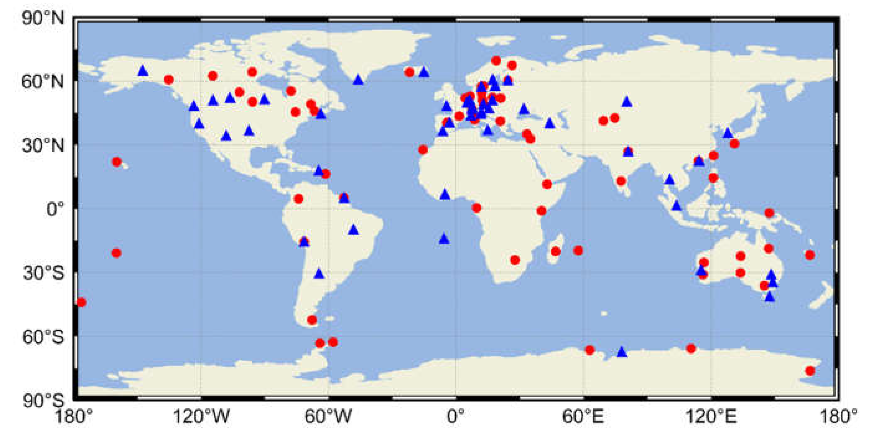
Figure 1 shows the distribution of stations and none of the stations for PPP experiment are used for deriving the satellite clocks. Thereafter, analysis of the residuals of network processing and satellite and receiver code biases are conducted. Finally, the estimated satellite clocks are compared with the IGS final products and applied in a pseudo-kinematic PPP procedure to evaluate their performance.
3.1. Residual Analysis
Processing residuals are important indicators that reflect the consistency between the observations and the function model [
8]. In this study, four models introduced in
Section 2 are employed for satellite clock estimation, and the difference between them is the processing strategy of code biases.
The time series of the root mean square (RMS) of the code residuals for different models on DOY 031 are shown in
Figure 2. Obviously, the RMS values of code residuals of the four models are in a reasonable range and very close, but there are still slight differences. In order to compare the residuals of each model, the mean RMS values are summarized in
Table 2.
As shown in
Table 2, if code biases are extracted in satellite clock estimation, the mean RMS values for code residuals will be reduced, which indicates that the time-varying part of the code biases are driven into the code residuals of the Undifferenced model. However, it does not mean that the code residuals contain all the time-varying code biases as in Equation (1), because some time-varying code biases may be absorbed by other parameters, such as clocks.
In addition, it can be seen from
Table 2 that the mean RMS value decreases from 1.033 to 0.997 m after extracting RCBs, while the mean RMS value only decreases to 1.014 m after extracting SCBs, which means that the time-varying characteristics of RCBs in the Undifferenced model code residuals are stronger than that of SCBs.
Theoretically, the Undifferenced-SRCB model should have the smallest mean RMS value, but it is not the case, as shown in
Table 2, which may be caused by too many constraints on the model.
The time series of the RMS of the phase residuals for different models on DOY 031 are shown in
Figure 3. The phase residuals of the four models are approximately equal, which indicates that the code bias extraction does not affect the residuals of phase equation. It should be noted that this does not mean that the code biases will not affect other parameters of the phase equation [
25].
3.2. Code Bias Analysis
Compared with the residual analysis, the direct analysis of code biases can better reflect their time-varying characteristics.
Figure 4 and
Figure 5 show the SCB time series extracted from the Undifferenced-SCB and Undifferenced-SRCB models, respectively. For the convenience of analysis, only six satellites are displayed, and the time series of each satellite is shifted to different degrees. As shown in the two figures, the time-varying code biases of the same satellite extracted using different models are consistent, which indicates that the excessive constraints imposed on the Undifferenced-SRCB model do not significantly damage the time-varying characteristics of the SCB.
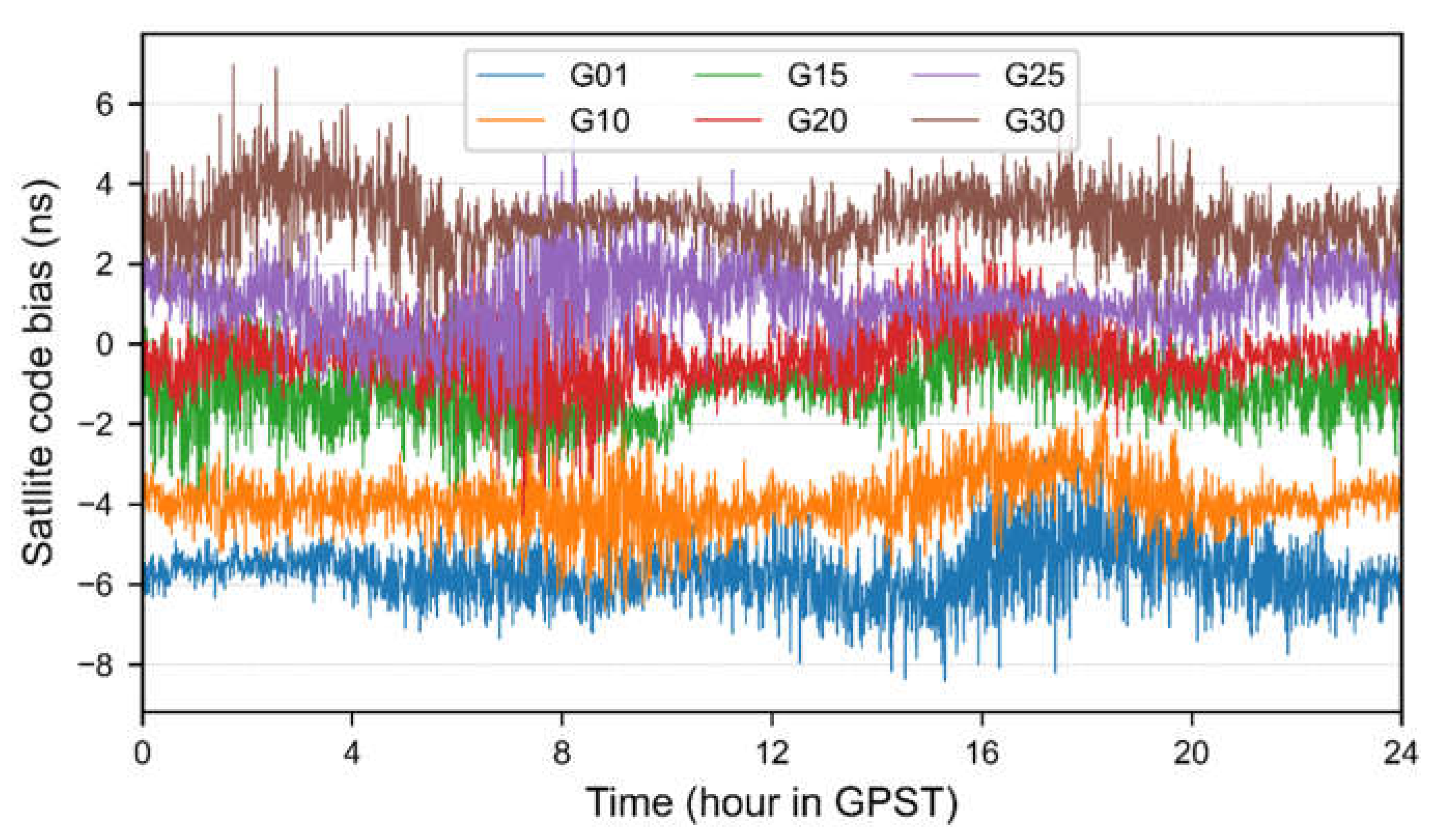
Though SCBs are contaminated by code noises due to the low accuracy of code observables, it can be found that SCBs appear in a peak-to-peak range of about 3 ns, as shown in
Figure 4. If those time-varying SCBs are driven into estimated satellite clocks, it will significantly damage the stability of clocks and reduce the accuracy of PPP at the user end.
Additionally, the RCB time series extracted from the Undifferenced-RCB and Undifferenced-SRCB models are also displayed in
Figure 6 and
Figure 7. For the convenience of analysis, only six receivers are displayed, and the time series of each receiver is shifted to different degrees. Compared with
Figure 6, the white noise characteristic of the RCB in
Figure 7 is destroyed, and the constraint of Equation (15) should be responsible for this. Different from SCBs, the variation of the RCB with time is more severe. Therefore, if those biases are not driven into code residuals such as Equation (2), it will bring adverse effects on the estimated parameters [
25].
3.3. Satellite Clock Validation
In order to assess the influence of different code bias extraction models on the stability of satellite clocks after the start of estimation, the satellite clocks are compared with the IGS final products. In this assessment, the RMS and standard deviation (STD) values for each satellite are calculated. The RMS values reflect the deviation degree of estimated clocks relative to the IGS, and the STD values represent the quality and stability of clocks.
Figure 8 shows the RMS and STD values of clock estimates compared with the IGS final products on DOY 031. Obviously, the RMS and STD values of the Undifferenced model are more consistent with the Undifferenced-RCB model, and the Undifferenced-SCB is closer to the Undifferenced-SRCB model, which indicates that the RCBs do not damage the quality of satellite clocks. Additionally, the mean RMS and STD values of the clock estimates displayed in
Figure 8 are given in
Table 3, which also confirms the above conclusion.
It can also be seen from
Figure 8 and
Table 3 that if the SCBs are extracted during the clock estimation process, the STD values of the satellite clocks decrease, but the RMS values increase at the same time, which means that the quality and stability of the satellite clocks are improved and the relative biases between the estimated and IGS clocks become larger. Obviously, the SCBs contained in IGS clocks are responsible for the increase in the RMS. It is worth noting that, the stability of IGS clocks is not destroyed by time-varying SCBs; therefore, those SCBs are likely to be driven into the code residuals such as Equation (2). Then, we can infer that the reason for the instability of clocks estimated using the Undifferenced model is that the time-varying SCBs are assimilated by the satellite clocks. Moreover, it is a time-consuming process to drive the time-varying SCBs into the code residuals; therefore, we extract SCBs directly to accelerate the convergence and stabilization of clocks.
Considering that SCBs are the main factors that damage the stability of satellite clocks, then only the Undifferenced and Undifferenced-SCB are compared in the following.
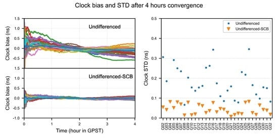
Figure 9 shows the biases of estimated satellite clocks with respect to the IGS final clocks. Compared with the Undifferenced model, the satellite clocks without SCBs have a faster convergence speed and are more stable. In particular, the satellite clock bias of the Undifferenced model, represented by the blue line, is changed by about 0.5 ns from the 12 h to the 20 h, but it is not the case in the Undifferenced-SCB model. The accuracy of the satellite clocks estimated using the above two models in one week is shown in
Table 4. As expected, the RMS of the Undifferenced-SCB model is larger than that of the Undifferenced model. After SCBs’ extraction, the mean STD of the clocks decreases from 0.15 to 0.07 ns.
3.4. Kinematic PPP Validation
Although extracting SCBs can improve the quality and stability of satellite clocks at the beginning of estimation, if these biases are not considered in PPP, the positioning accuracy will be seriously damaged. Unfortunately, as discussed in
Section 3.2, SCBs are contaminated by code noises; therefore, they cannot be used as the corrections in PPP. In this study, we increase the noises of code observations to realize the application of satellite clocks without SCBs in PPP.
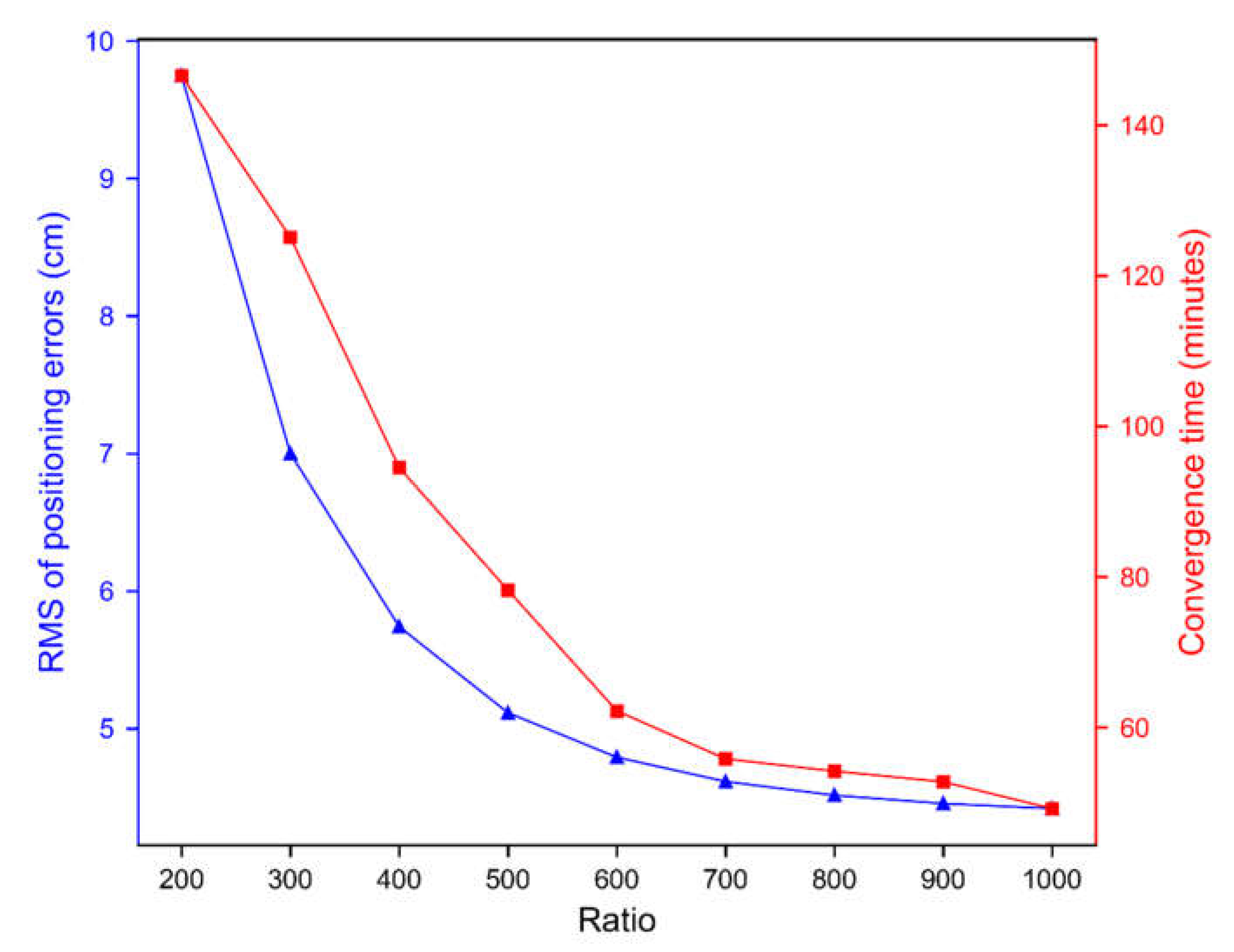
Here, we define Ratio as the prior noise ratio of the code observations and the phase observations. Generally, the Ratio is set to 100, which means that if the prior noise of the phase observations is 0.003 m, then the noise of the code observations is 0.3 m. The observation data on DOY 031 of 57 stations distributed in
Figure 1 are used for PPP with different ratio values. The positioning accuracy and convergence time are investigated to determine the appropriate Ratio.
Figure 10 shows the statistical results, where the positioning error is a three-dimensional error and the convergence time is defined as the time required to attain a three-dimensional positioning error less than 15 cm and keep at least for 10 epochs [
32]. The positioning accuracy is poor when the Ratio is 100; therefore, it is not plotted in the figure.
It can be seen from
Figure 10 that with the increase in the Ratio, the positioning accuracy is improved, and the convergence time is reduced. When the Ratio is greater than 700, the positioning performance is not significantly improved. In addition, large observation noises are not conducive to the convergence of PPP. Therefore, we set the Ratio to 700 when the satellite clocks estimated using the Undifferenced-SCB model are applied to carry out PPP experiments, and set the Ratio to 100 when the satellite clocks estimated using the Undifferenced model or the IGS final clocks are used. Then, the above three kinds of clocks are used in PPP to evaluate the effectiveness of Undifferenced-SCB clocks. It should be noted that in order to prove the advantage of the Undifferenced-SCB model at the beginning of the estimation, satellite clocks estimated using the Undifferenced and Undifferenced-SCB models used in PPP do not converge in advance; therefore, the PPP solutions obtained by using the IGS clocks should have obvious positioning performance advantages.
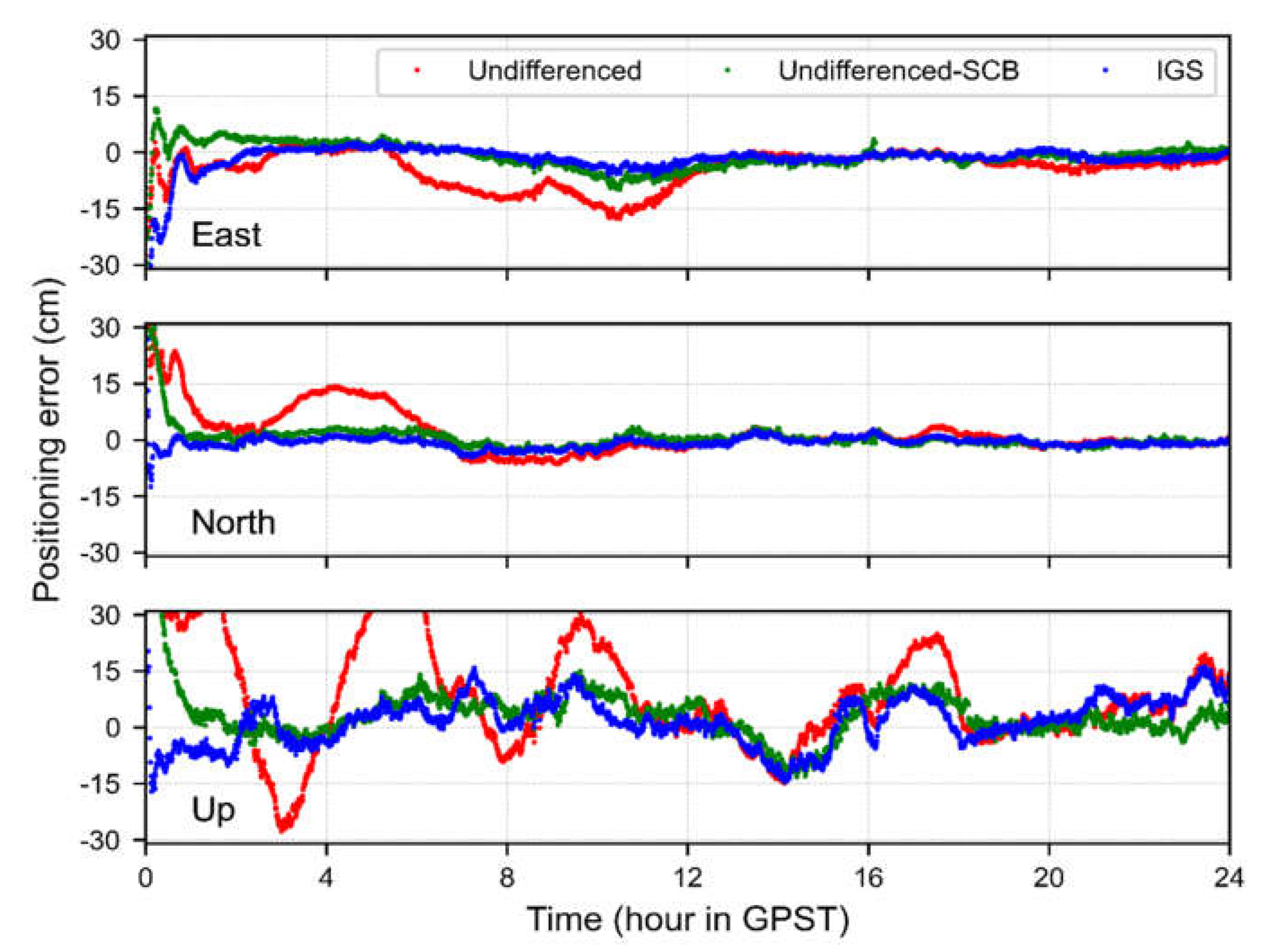
Figure 11 shows the time series of the positioning errors for station ABPO as an example. Obviously, compared with the Undifferenced solution, the Undifferenced-SCB offers a better positioning and convergence performance. Moreover,
Figure 12 shows the RMS of the positioning errors with IGS solutions in contrast to those with the Undifferenced and Undifferenced-SCB solutions for each station from DOY 031 to 037. Each dot in the figure represents one station. There is no doubt that IGS solutions have the most effective performance. In addition, the positioning performance of the Undifferenced-SCB solutions is closer to the IGS than that of the Undifferenced solutions.
Table 5 shows the mean positioning errors of all the stations in one week after two hours of convergence. For the Undifferenced solution, the RMSs of the positioning errors are 6.61, 4.49 and 12.14 cm in east, north and up directions, while the RMSs of the Undifferenced-SCB solution can reduced by 43.0, 23.4 and 35.9 %, respectively.
In addition to positioning accuracy, the convergence speed of different solutions has also been assessed.
Figure 13 shows the mean convergence time of all the stations in a single day. Obviously, significant convergence improvements can be found in the Undifferenced-SCB solutions with respect to the Undifferenced solutions, and the convergence time of the former is half that of the latter. Considering that clock estimation starts from 0 h in each day, the convergence time gap between the Undifferenced-SCB and the IGS solutions is reasonable.
4. Discussion
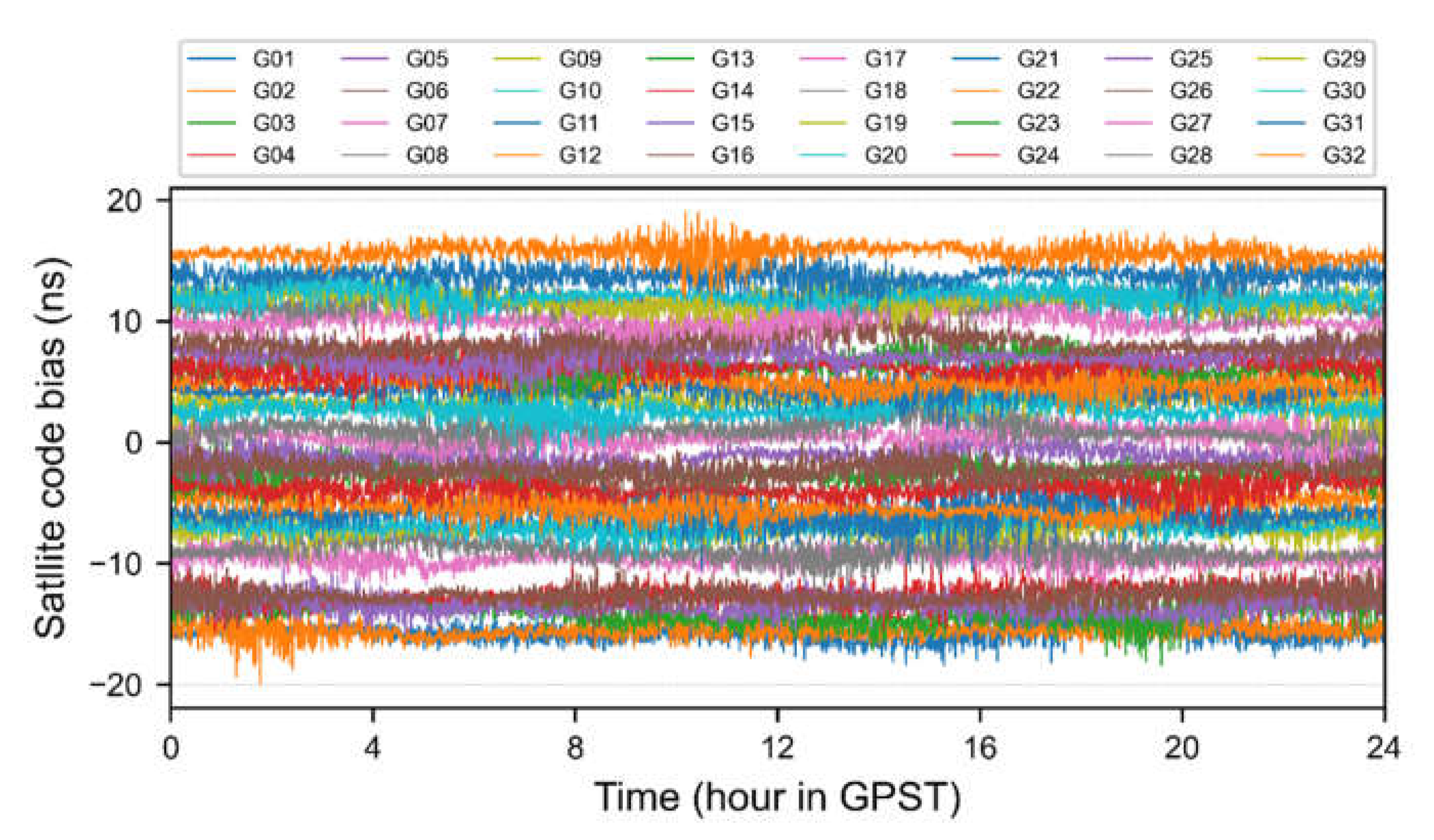
Figure 14 shows the SCB time series extracted from the Undifferenced-SCB model. For the convenience of observation, the time series of each satellite is shifted to different degrees. As shown in the figure, although those SCBs are not stable constants, their time-varying characteristics are not dramatic. Therefore, the constant part of the SCB is usually absorbed by the satellite clock in estimation, and the time-varying part is driven into the code residual to generate stable clock products. On the one hand, the time-varying part of the SCB is not dramatic, and it can be driven into the code residual after a long time of convergence. On the other hand, it is also to eliminate the rank deficiency and obtain the full rank model. However, when the filtering system needs to converge again, the time-varying SCB will seriously damage the convergence speed and stability of the clocks.
The key to accelerating the convergence of the satellite clock to a stable state is to get rid of the disturbance of the time-varying part of the SCB. Additionally, there are two methods to solve this problem. The first is that a robust filtering model needs to be constructed to accelerate the time-varying part of the SCB being driven to code residual. The advantage of this method is that the estimated satellite clocks are consistent with that of the IGS, which avoids trouble at the user end. However, how to build a robust filtering model needs more research. The second method is to extract the SCB directly. The advantage of this method is that it can directly avoid the adverse effects of SCBs and other unmodeled satellite related errors on clocks, but the influence of SCB should be considered in PPP at the user end. The latter method is adopted in this study.
At the user end, the full rank SCB extraction model cannot be constructed, as in the network processing. In addition, due to the contamination of the code observation, the SCB extracted from network processing cannot be used as a correction in PPP directly. In this study, the weight of the code equation is reduced to eliminate the negative effect of SCB, and experiments show that this is a simple and feasible strategy.
5. Conclusions
It usually takes a long time for clocks to converge when estimating satellite clocks based on an undifferenced IF model. Moreover, the clocks cannot reach stability in a short time after convergence. For this reason, we investigated the influence of time-varying code biases on the stability of satellite clocks and proposed a new clock estimation method considering SCBs.
Clock estimation and PPP experiments were carried out to verify the effectiveness of the new method. By comparing the results of the Undifferenced and Undifferenced-SCB models, the following conclusions can be drawn. First, the time-varying characteristics of SCBs can be determined using the Undifferenced-SCB model, and they are the main factors that cause the instability of satellite clocks. Then, different from the original undifferenced method, the clocks estimated using the new method are free of the adverse effects of SCBs and can converge and reach stability in a short time. Finally, the clocks estimated using the new method can significantly improve the convergence speed and positioning accuracy of PPP, that is, the convergence speed can be doubled, and the positioning errors can be reduced by 20–45%.
Since the SCBs are not corrected to code observables in PPP, the weight of the code equations is reduced to eliminate the negative effects of SCBs. Although this is effective, it is only a compromise strategy. On the one hand, the code equations with large noise reduce the convergence speed. On the other hand, the filter may converge to the wrong states due to the high weight of the phase equations, which leads to poor positioning solutions. Therefore, more attention should be paid to how to apply the satellite clocks without SCBs to PPP in the future.
Author Contributions
S.L. provided the initial idea and wrote the manuscript; S.L. and Y.Y. designed and performed the research; Y.Y. helped with the writing and partially financed the research. All authors have read and agreed to the published version of the manuscript.
Funding
This work was supported by the National Key Research Program of China “Collaborative Precision Positioning Project” (No. 2016YFB0501900) funded by the Ministry of Science and Technology of the People’s Republic of China. The second author acknowledges the Lu Jiaxi International Team program supported by the K.C. Wong Education Foundation and CAS.
Data Availability Statement
The datasets analyzed in this study can be made available by the corresponding author on request.
Acknowledgments
The authors would like to acknowledge the IGS for providing the observation data and precise products.
Conflicts of Interest
The authors declare no conflict of interest.
References
- Zumberge, J.F.; Watkins, M.M.; Webb, F.H. Characteristics and Applications of Precise GPS Clock Solutions Every 30 s. Navigation 1997, 44, 449–456. [Google Scholar] [CrossRef]
- Kouba, J.; Héroux, P. Precise Point Positioning Using IGS Orbit and Clock Products. GPS Solut. 2001, 5, 12–28. [Google Scholar] [CrossRef]
- Hauschild, A.; Montenbruck, O. Kalman-filter-based GPS clock estimation for near real-time positioning. GPS Solut. 2009, 13, 173–182. [Google Scholar] [CrossRef]
- Bock, H.; Dach, R.; Jäggi, A.; Beutler, G. High-rate GPS clock corrections from CODE: Support of 1 Hz applications. J. Geod. 2009, 83, 1083–1094. [Google Scholar] [CrossRef] [Green Version]
- Zhang, X.; Li, X.; Guo, F. Satellite clock estimation at 1 Hz for realtime kinematic PPP applications. GPS Solut. 2011, 15, 315–324. [Google Scholar] [CrossRef]
- Ge, M.; Chen, J.; Douša, J.; Gendt, G.; Wickert, J. A computationally efficient approach for estimating high-rate satellite clock corrections in realtime. GPS Solut. 2012, 16, 9–17. [Google Scholar] [CrossRef]
- Chen, Y.; Yuan, Y.; Zhang, B.; Liu, T.; Ding, W.; Ai, Q. A modified mix-differenced approach for estimating multi-GNSS real-time satellite clock offsets. GPS Solut. 2018, 22, 72. [Google Scholar] [CrossRef]
- Liu, T.; Zhang, B.; Yuan, Y.; Zha, J.; Zhao, C. An efficient undifferenced method for estimating multi-GNSS high-rate clock corrections with data streams in real time. J. Geod. 2019, 93, 1435–1456. [Google Scholar] [CrossRef]
- Zhang, W.; Lou, Y.; Gu, S.; Shi, C.; Haase, J.S.; Liu, J. Joint estimation of GPS/BDS real-time clocks and initial results. GPS Solut. 2016, 20, 665–676. [Google Scholar] [CrossRef]
- Chen, Y.; Yuan, Y.; Ding, W.; Zhang, B.; Liu, T. GLONASS pseudorange inter-channel biases considerations when jointly estimating GPS and GLONASS clock offset. GPS Solut. 2017, 21, 1525–1533. [Google Scholar] [CrossRef]
- Ai, Q.; Yuan, Y.; Zhang, B.; Xu, T.; Chen, Y. Refining GPS/GLONASS Satellite Clock Offset Estimation in the Presence of Pseudo-Range Inter-Channel Biases. Remote Sens. 2020, 12, 1821. [Google Scholar] [CrossRef]
- Hauschild, A.; Montenbruck, O.; Steigenberger, P. Short-term analysis of GNSS clocks. GPS Solut. 2013, 17, 295–307. [Google Scholar] [CrossRef]
- Hadas, T.; Bosy, J. IGS RTS precise orbits and clocks verification and quality degradation over time. GPS Solut. 2015, 19, 93–105. [Google Scholar] [CrossRef] [Green Version]
- Li, X.; Ge, M.; Dai, X.; Ren, X.; Fritsche, M.; Wickert, J.; Schuh, H. Accuracy and reliability of multi-GNSS real-time precise positioning: GPS, GLONASS, BeiDou, and Galileo. J. Geod. 2015, 89, 607–635. [Google Scholar] [CrossRef]
- Kazmierski, K.; Sośnica, K.; Hadas, T. Quality assessment of multi-GNSS orbits and clocks for real-time precise point positioning. GPS Solut. 2018, 22, 11. [Google Scholar] [CrossRef] [Green Version]
- Kazmierski, K.; Zajdel, R.; Sośnica, K. Evolution of orbit and clock quality for real-time multi-GNSS solutions. GPS Solut. 2020, 24, 1–12. [Google Scholar] [CrossRef]
- Håkansson, M.; Jensen, A.B.O.; Horemuz, M.; Hedling, G. Review of code and phase biases in multi-GNSS positioning. GPS Solut. 2017, 21, 849–860. [Google Scholar] [CrossRef] [Green Version]
- Collins, P.; Bisnath, S.; Lahaye, F.; Héroux, P. Undifferenced GPS Ambiguity Resolution Using the Decoupled Clock Model and Ambiguity Datum Fixing. Navig. J. Inst. Navig. 2010, 57, 123–135. [Google Scholar] [CrossRef] [Green Version]
- Wen, Z.; Henkel, P.; Günther, C. Multi-Stage Satellite Phase and Code Bias Estimation. Automatika 2012, 53, 373–381. [Google Scholar] [CrossRef]
- Coster, A.; Williams, J.; Weatherwax, A.; Rideout, W.; Herne, D. Accuracy of GPS total electron content: GPS receiver bias temperature dependence. Radio Sci. 2013, 48, 190–196. [Google Scholar] [CrossRef]
- Wanninger, L.; Sumaya, H.; Beer, S. Group delay variations of GPS transmitting and receiving antennas. J. Geod. 2017, 91, 1099–1116. [Google Scholar] [CrossRef] [Green Version]
- McCaffrey, A.M.; Jayachandran, P.T.; Themens, D.R.; Langley, R.B. GPS receiver code bias estimation: A comparison of two methods. Adv. Space Res. 2017, 59, 1984–1991. [Google Scholar] [CrossRef]
- Zhang, B.; Liu, T.; Yuan, Y. GPS receiver phase biases estimable in PPP-RTK networks: Dynamic characterization and impact analysis. J. Geod. 2018, 92, 659–674. [Google Scholar] [CrossRef]
- Wang, J.; Huang, G.; Yang, Y.; Zhang, Q.; Gao, Y.; Zhou, P. Mitigation of short-term temporal variations of receiver code bias to achieve increased success rate of ambiguity resolution in PPP. Remote Sens. 2020, 12, 796. [Google Scholar] [CrossRef] [Green Version]
- Zhang, B.; Zhao, C.; Odolinski, R.; Liu, T. Functional model modification of precise point positioning considering the time-varying code biases of a receiver. Satell. Navig. 2021, 2, 11. [Google Scholar] [CrossRef]
- Wu, J.T.; Wu, S.C.; Hajj, G.A.; Bertiger, W.I.; Lichten, S.M. Effects of antenna orientation on GPS carrier phase. Proc. Adv. Astronaut. Sci. 1992, 76. [Google Scholar]
- Geng, J.; Chen, X.; Pan, Y.; Zhao, Q. A modified phase clock/bias model to improve PPP ambiguity resolution at Wuhan University. J. Geod. 2019, 93, 2053–2067. [Google Scholar] [CrossRef]
- Dach, R.; Lutz, S.; Walser, P.; Fridez, P. (Eds.) Bernese GNSS Software Version 5.2; University of Bern, Bern Open Publishing: Bern, Switzerland, 2015. [Google Scholar]
- Zhao, C.; Yuan, Y.; Zhang, B.; Li, M. Ionosphere Sensing With a Low-Cost, Single-Frequency, Multi-GNSS Receiver. IEEE Trans. Geosci. Remote Sens. 2019, 57, 881–892. [Google Scholar] [CrossRef]
- Saastamoinen, J. Contributions to the theory of atmospheric refraction. Bull. Géodésique 1972, 105, 279–298. [Google Scholar] [CrossRef]
- Niell, A.E. Global mapping functions for the atmosphere delay at radio wavelengths. J. Geophys. Res. Solid Earth 1996, 101, 3227–3246. [Google Scholar] [CrossRef]
- Hu, J.; Zhang, X.; Li, P.; Ma, F.; Pan, L. Multi-GNSS fractional cycle bias products generation for GNSS ambiguity-fixed PPP at Wuhan University. GPS Solut. 2020, 24, 15. [Google Scholar] [CrossRef]
Figure 1.
Overview of the experimental stations. Red circles denote 70 stations for satellite clock estimation, and blue triangles denote 57 stations for PPP experiment. The observation data are obtained from the IGS MGEX networks.
Figure 1.
Overview of the experimental stations. Red circles denote 70 stations for satellite clock estimation, and blue triangles denote 57 stations for PPP experiment. The observation data are obtained from the IGS MGEX networks.
Figure 2.
Time series of RMS of the code residuals for different models on DOY 031.
Figure 2.
Time series of RMS of the code residuals for different models on DOY 031.
Figure 3.
Time series of RMS of the phase residuals for different models on DOY 031.
Figure 3.
Time series of RMS of the phase residuals for different models on DOY 031.
Figure 4.
Time series of SCBs extracted by Undifferenced-SCB model on DOY 031.
Figure 4.
Time series of SCBs extracted by Undifferenced-SCB model on DOY 031.
Figure 5.
Time series of SCBs extracted by Undifferenced-SRCB model on DOY 031.
Figure 5.
Time series of SCBs extracted by Undifferenced-SRCB model on DOY 031.
Figure 6.
Time series of RCBs extracted by Undifferenced-RCB model on DOY 031.
Figure 6.
Time series of RCBs extracted by Undifferenced-RCB model on DOY 031.
Figure 7.
Time series of RCBs extracted by Undifferenced-SRCB model on DOY 031.
Figure 7.
Time series of RCBs extracted by Undifferenced-SRCB model on DOY 031.
Figure 8.
RMS and STD values of clock estimates compared with the IGS final products on DOY 031. The mean values are also plotted near the right edge of each panel. G01 is the reference satellite.
Figure 8.
RMS and STD values of clock estimates compared with the IGS final products on DOY 031. The mean values are also plotted near the right edge of each panel. G01 is the reference satellite.
Figure 9.
Time series of the clock biases with respect to the IGS final products on DOY 031. Different colors correspond to different satellites, and mean values are removed.
Figure 9.
Time series of the clock biases with respect to the IGS final products on DOY 031. Different colors correspond to different satellites, and mean values are removed.
Figure 10.
Comparison of positioning accuracy and convergence time with different ratio values on DOY 031.
Figure 10.
Comparison of positioning accuracy and convergence time with different ratio values on DOY 031.
Figure 11.
Time series of the positioning errors using different satellite clocks for station ABPO on DOY 031.
Figure 11.
Time series of the positioning errors using different satellite clocks for station ABPO on DOY 031.
Figure 12.
RMS of positioning errors for different PPP solutions when compared to IGS weekly solutions at 57 stations from DOY 031 to 037.
Figure 12.
RMS of positioning errors for different PPP solutions when compared to IGS weekly solutions at 57 stations from DOY 031 to 037.
Figure 13.
The mean convergence time for various PPP solutions from DOY 031 to 037.
Figure 13.
The mean convergence time for various PPP solutions from DOY 031 to 037.
Figure 14.
Time series of all GPS SCBs extracted using Undifferenced-SCB model on DOY 031.
Figure 14.
Time series of all GPS SCBs extracted using Undifferenced-SCB model on DOY 031.
Table 1.
Detailed strategies for satellite clock estimation and PPP.
Table 1.
Detailed strategies for satellite clock estimation and PPP.
| Items | Strategies |
|---|
| Observations | GPS code and phase |
| Priori noises | 0.3 and 0.003 m for raw code and phase observations in clock estimation, respectively; in PPP, 0.003 m for phase and priori noises for code discussed in Section 3 |
| Cut-off elevation | 10° |
| Differential code bias | CODE P1-C1 products |
| Relativistic effect | Corrected |
| Phase wind-up | Corrected |
| PCOs/PCVs | igs14.atx |
| Tidal displacements | Solid earth tide, ocean tide loading and pole tide |
| Station coordinates | Fixed to IGS weekly solutions in clock estimation, and estimated as white noises in PPP |
| Satellite orbits | Fixed to IGS final products |
| Earth rotation effects | Fixed to IGS final products |
| Receiver clocks | Estimated as white noises |
| Satellite clocks | Estimated as white noises in clock estimation, and fixed to estimated clocks or IGS final products in PPP |
| Zenith troposphere delays | Estimated as random-walk noises () with respect to Saastamoinen model 1, and NMF 2 is used |
| Ambiguities | Estimated as constants over each continuous session |
| Code biases | Estimated as white noises |
| Estimator | Least square filter |
Table 2.
The mean RMS values for code residuals.
Table 2.
The mean RMS values for code residuals.
| Models | Code Residuals (m) |
|---|
| Undifferenced | 1.033 |
| Undifferenced-SCB | 1.014 |
| Undifferenced-RCB | 0.997 |
| Undifferenced-SRCB | 0.999 |
Table 3.
The mean RMS and STD of clock estimates by different models when compared to the IGS final products on DOY 031.
Table 3.
The mean RMS and STD of clock estimates by different models when compared to the IGS final products on DOY 031.
| Models | RMS (ns) | STD (ns) |
|---|
| Undifferenced | 0.73 | 0.15 |
| Undifferenced-SCB | 1.24 | 0.06 |
| Undifferenced-RCB | 0.72 | 0.15 |
| Undifferenced-SRCB | 1.33 | 0.08 |
Table 4.
The RMS and STD of clock estimates using different models when compared to the IGS final products from DOY 031 to 037.
Table 4.
The RMS and STD of clock estimates using different models when compared to the IGS final products from DOY 031 to 037.
| DOY | Undifferenced Model | Undifferenced-SCB Model |
|---|
| RMS (ns) | STD (ns) | RMS (ns) | STD (ns) |
|---|
| 031 | 0.73 | 0.15 | 1.24 | 0.06 |
| 032 | 0.69 | 0.14 | 0.85 | 0.07 |
| 033 | 0.71 | 0.14 | 0.82 | 0.09 |
| 034 | 0.73 | 0.15 | 1.12 | 0.07 |
| 035 | 0.70 | 0.15 | 0.85 | 0.08 |
| 036 | 0.70 | 0.15 | 1.13 | 0.08 |
| 037 | 0.71 | 0.14 | 0.75 | 0.06 |
| Mean | 0.71 | 0.15 | 0.97 | 0.07 |
Table 5.
The mean RMS (cm) for different PPP solutions when compared to IGS weekly solutions at 57 stations from DOY 031 to 037.
Table 5.
The mean RMS (cm) for different PPP solutions when compared to IGS weekly solutions at 57 stations from DOY 031 to 037.
| PPP Solutions | East | North | Up |
|---|
| IGS solution | 2.43 | 2.03 | 5.36 |
| Undifferenced solution | 6.61 | 4.49 | 12.14 |
| Undifferenced-SCB solution | 3.77 | 3.44 | 7.78 |
| Publisher’s Note: MDPI stays neutral with regard to jurisdictional claims in published maps and institutional affiliations. |
© 2021 by the authors. Licensee MDPI, Basel, Switzerland. This article is an open access article distributed under the terms and conditions of the Creative Commons Attribution (CC BY) license (https://creativecommons.org/licenses/by/4.0/).


