A 3D Cascaded Spectral–Spatial Element Attention Network for Hyperspectral Image Classification

Abstract

Most traditional hyperspectral image (HSI) classification methods relied on hand-crafted or shallow-based descriptors, which limits their applicability and performance. Recently, deep learning has gradually become the mainstream method of HSI classification, because it can automatically extract deep abstract features for classification. However, it remains a challenge to learn more meaningful features for HSI classification from a small training sample set. In this paper, a 3D cascaded spectral–spatial element attention network (3D-CSSEAN) is proposed to solve this issue. The 3D-CSSEAN integrates the spectral–spatial feature extraction and attention area extraction for HSI classification. Two element attention modules in the 3D-CSSEAN enable the deep network to focus on primary spectral features and meaningful spatial features. All attention modules are implemented though several simple activation operations and elementwise multiplication operations. In this way, the training parameters of the network are not added too much, which also makes the network structure suitable for small sample learning. The adopted module cascading pattern not only reduces the computational burden in the deep network but can also be easily operated via plug–expand–play. Experimental results on three public data sets show that the proposed 3D-CSSEAN achieved comparable performance with the state-of-the-art methods.

1. Introduction

With the development of remote sensing technology, hyperspectral images (HSIs) have been of wide concern and gradually applied in many fields [1,2]. In the field of HSIs, as a fundamental task, HSI classification is a task of assigning category labels to each pixel in the HSI and has attracted more and more attention.

An HSI usually contains hundreds of spectral bands, so it has abundant spectral information in addition to the usual spatial information of the image. In the early stages of HSI classification, there were many works based on spectral or spatial characteristics [3]. Support vector machines (SVMs) were used to address the problem by using spectral information [4]. In the past ten years, many works were based on spectral–spatial feature learning for HSI classification [5,6]. The performance of sparse representation was improved by using the spatial neighborhood information of samples [7]. In [8], principal component analysis (PCA) was used for unsupervised extraction of spectral features and data dimensionality reduction, and edge-preserving features were obtained by edge-preserving filtering, and the resulting features were classified by an SVM classifier. A hierarchical subspace and ensemble learning algorithm was proposed to solve the problem of hyperspectral image classification, in which spectral–spatial features were also applied [9]. Although most of these methods based on spectral–spatial features have achieved better results than those based on spectral information alone, they usually rely on hand-crafted or shallow-based descriptors. Therefore, the robustness and classification accuracy of these traditional methods still need to be improved.

In recent years, deep learning has been widely adopted in HSI classification because of its advantage of automatically learning discrimination features from raw data [10]. Autoencoders (AEs) were applied to extract the deep features of the image in an unsupervised manner [11,12]. In [13], the spectral information of each pixel was regarded as a sequence, and sequence features were extracted by recurrent neural networks (RNNs) for HSI classification. In [14], AE and RNN were combined to construct a new network for HSI classification.

Convolutional neural networks (CNNs) have been widely used in the field of HSI classification because of the advantages of spatial extraction and weight sharing mechanisms [15,16]. In [17], 1D CNNs were employed to extract the spectral features for HSI classification. The spectral images in HSIs were treated as the channels of conventional images, and then 2D CNNs were designed to extract the spatial features for HSI classification [18]. A 3D CNN that combined spectral and spatial information was used for HSI classification [19]. A spectral–spatial residual network (SSRN) adopted a 3D CNN and residual connections to improve the classification accuracy [20]. Batch normalization (BN) was used to regularize the training process in SSRN, making the training processing of the deep learning model more efficient. A 3D CNN has advantages over a 1D CNN and a 2D CNN in simultaneously extracting spectral and spatial features, while it requires more computation. To reduce the computational burden of 3D CNNs, 3D and 2D CNNs were mixed in a hybrid network (HybridSN) for HSI classification [21]. Overall, deep spectral–spatial feature learning has become a new trend in the classification of HSIs. Among these deep learning methods, it is difficult to achieve satisfactory results with the existing unsupervised network methods. Although these deep learning methods trained in a supervised manner can obtain encouraging results, they usually require sufficient labelled samples for training. However, obtaining labelled samples of hyperspectral images often consumes a lot of human and material resources. Therefore, training a deep learning model for hyperspectral image classification with limited samples is still a challenge.

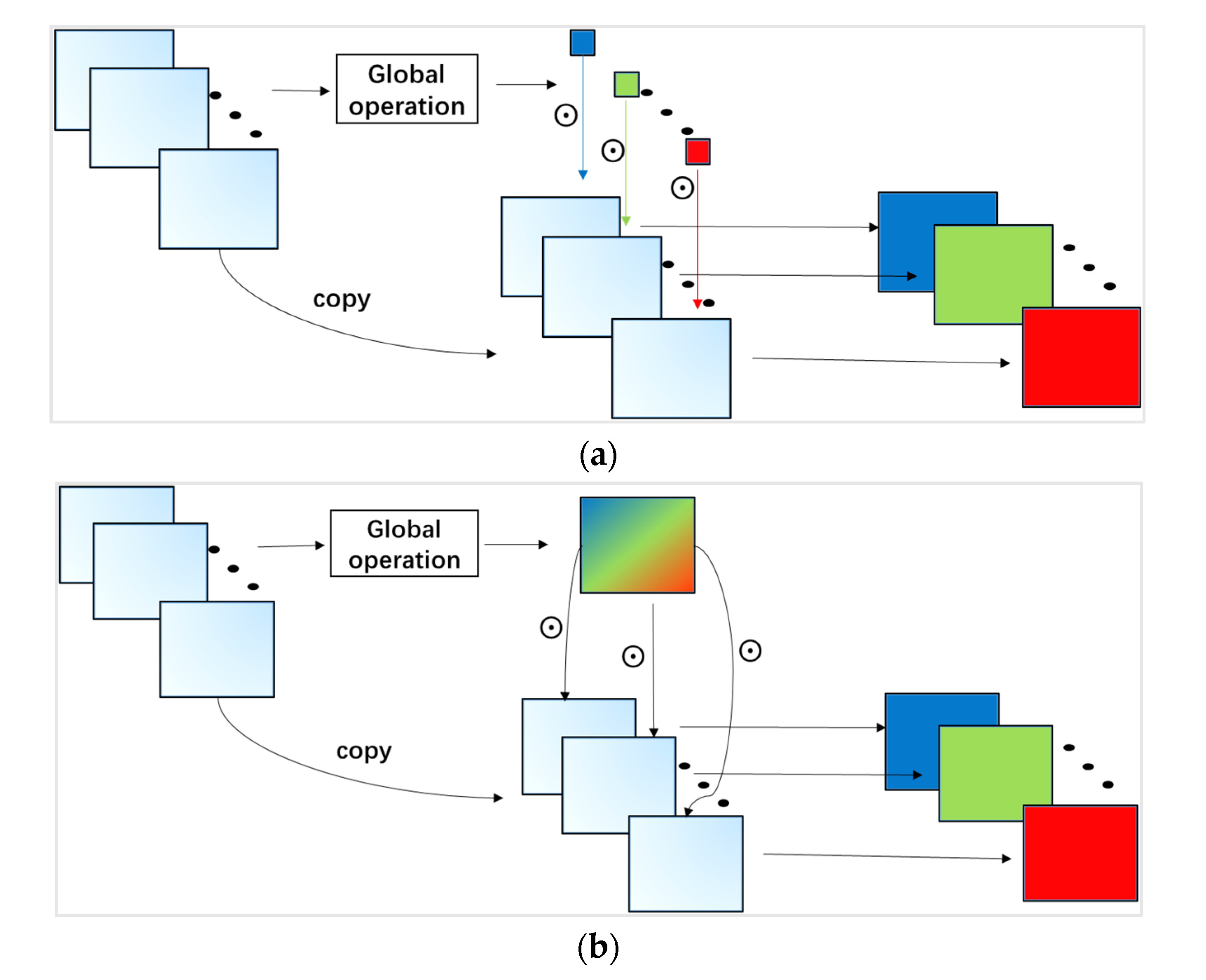
Recently, some deep learning methods have introduced the attention mechanism to alleviate these problems in HSI classification [22,23]. The attention mechanism is inspired by the human visual mechanism [24,25]. When people observe a scene, they always pay more attention to the area of interest to obtain more meaningful information. In [26], the global pooling operations in the spectral dimension and spatial dimension were used to assign the attention to the interesting features. In [27], the spatial correlation and spectral band correlation were used to compute the attention weights of feature learning. In [28], a cascaded dual-scale crossover network (CDSCN) was proposed for HSI classification, which can obtain the parts of interest in the images through the multiplication of dual branch features. These methods use different ways to obtain attention features, thereby improving the classification performance. In addition to these attention methods, there may be other ways to extract attention features.

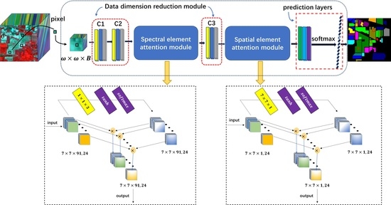
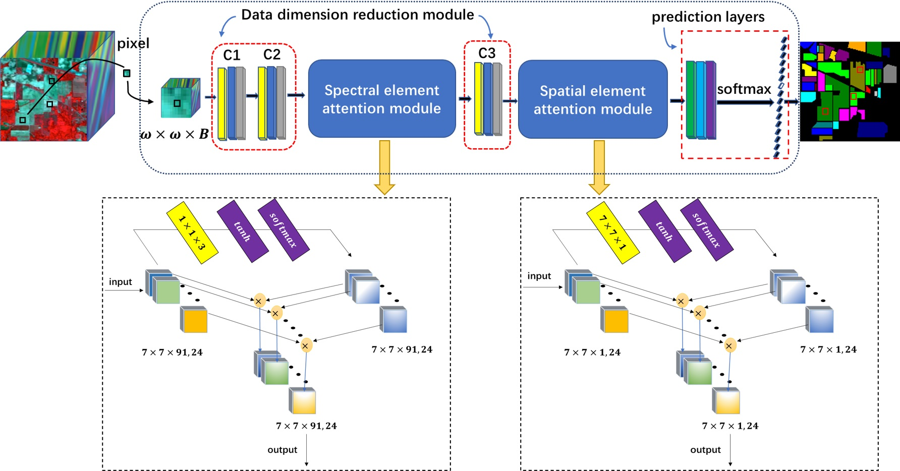
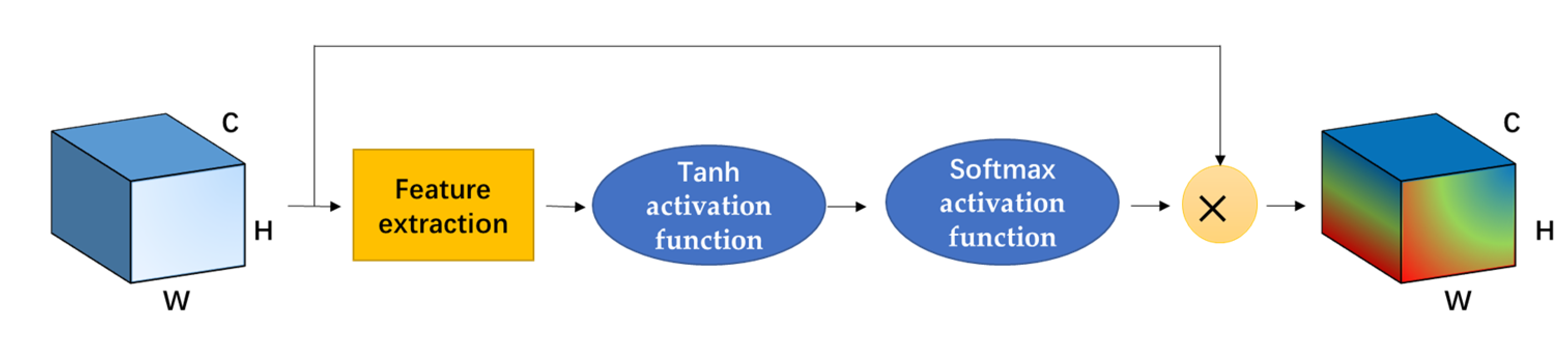
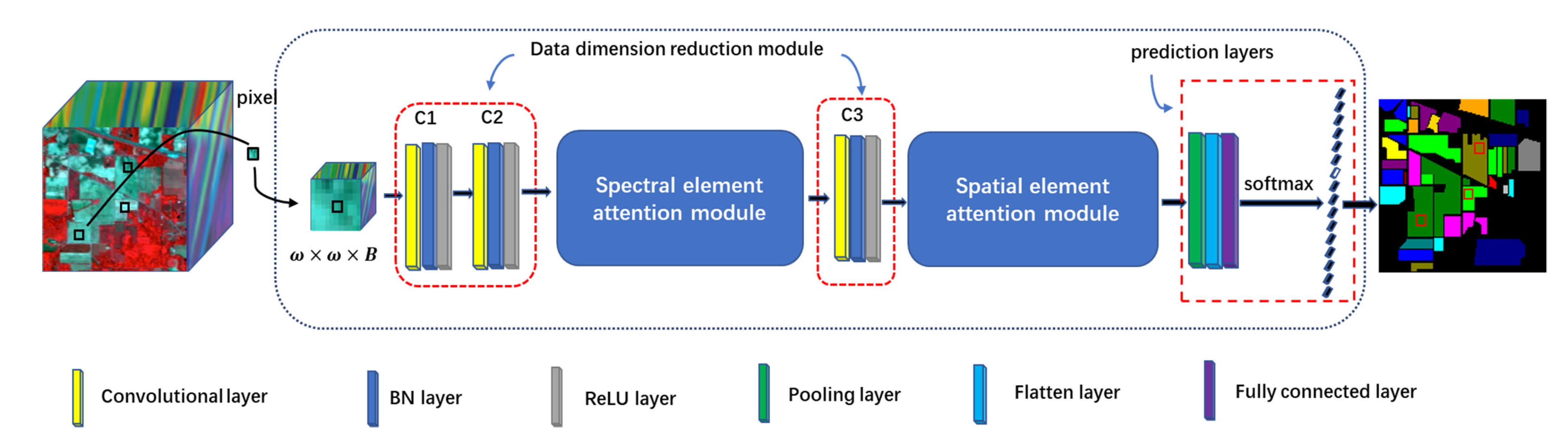
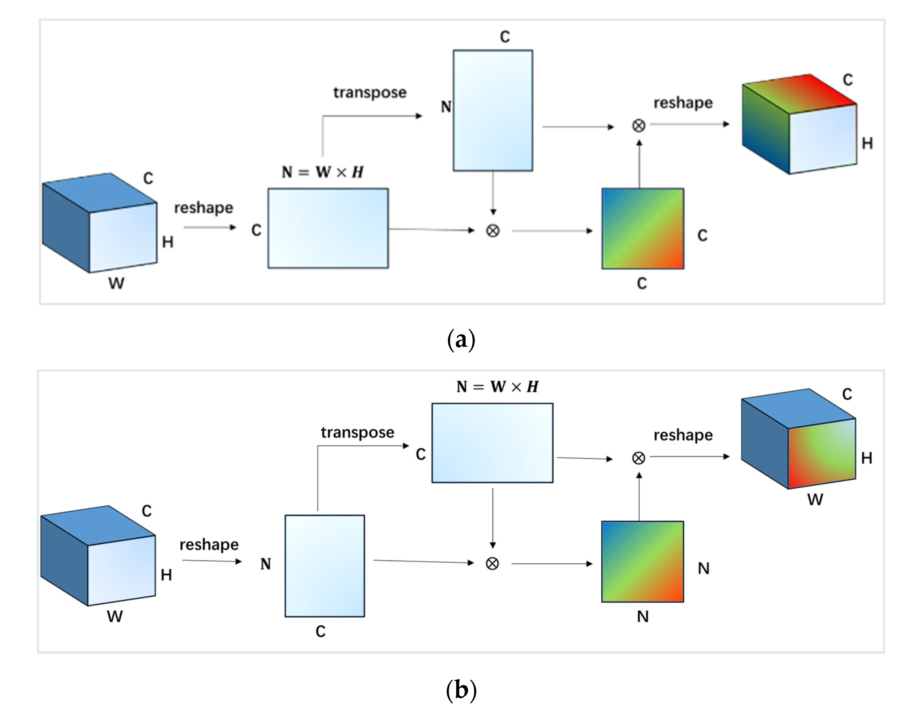
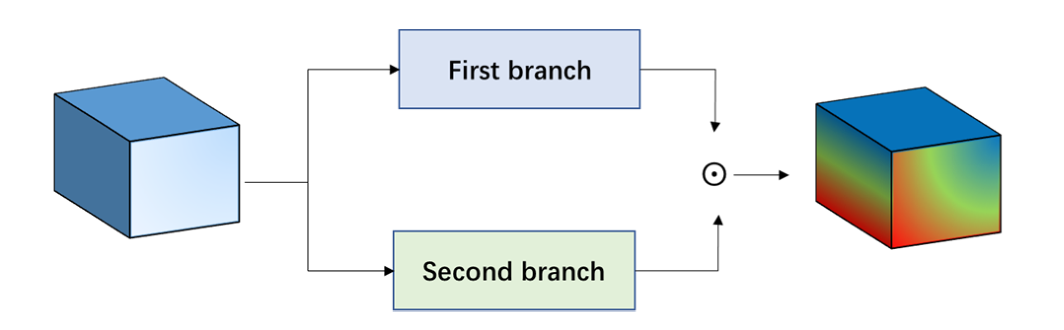
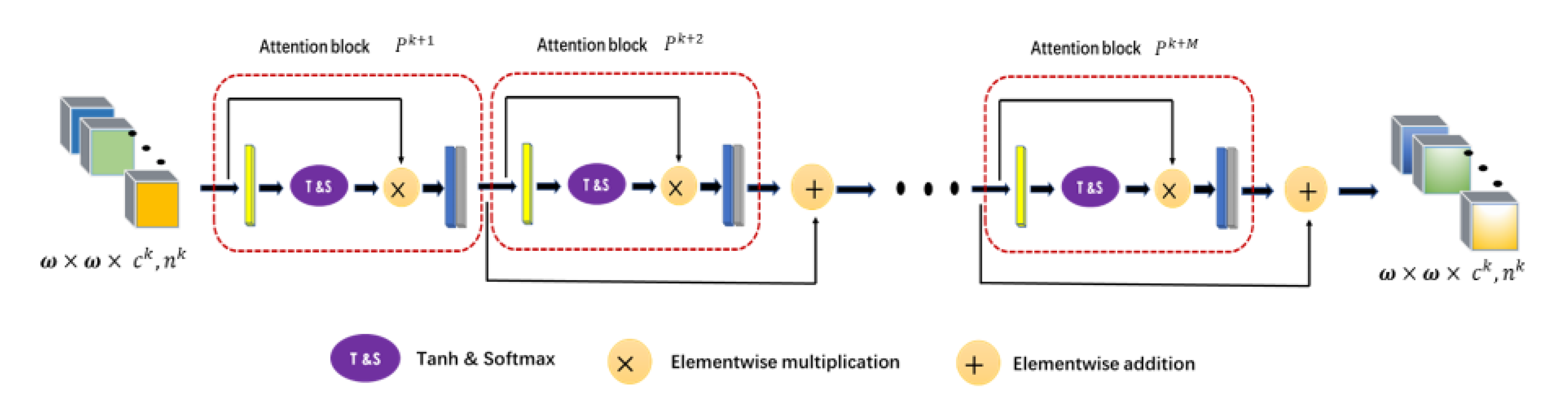
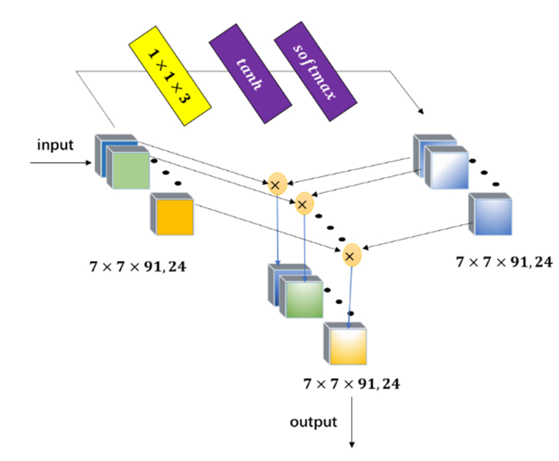
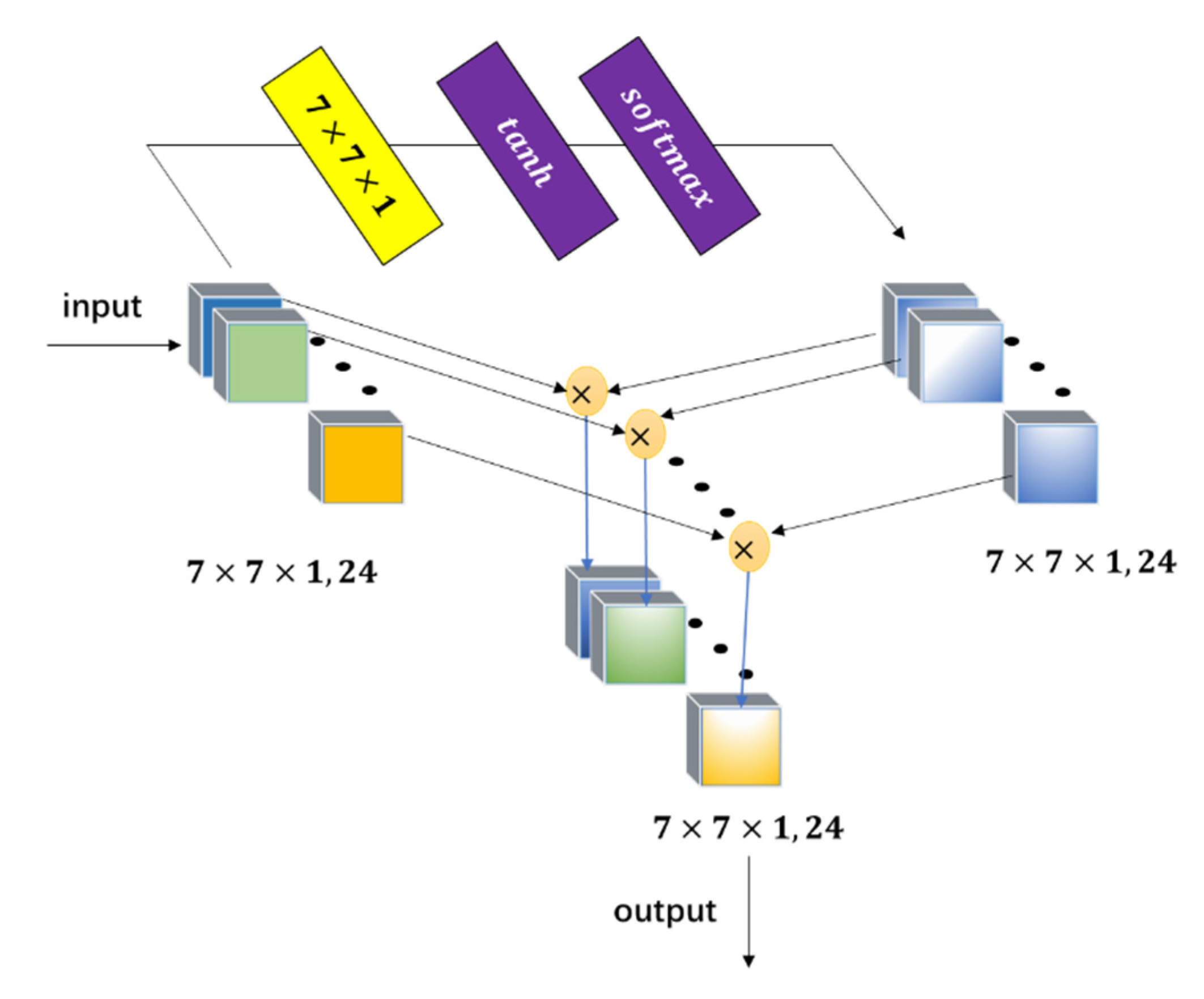
In this paper, a 3D cascaded spectral–spatial element attention network (3D-CSSEAN) is proposed for HSI classification. In 3D-CSSEAN, an element attention mechanism is used to extract spectral and spatial attention features, as shown in Figure 1. This method is different from the attention method mentioned above. It uses several activation functions to assign weights to all elements in the 3D feature tensor and obtains attention features through elementwise multiplication. The overall framework of 3D-CSSEAN is shown in Figure 2. It first uses convolution operations for data dimensionality reduction and shallow feature extraction. Then two attention modules are used to extract attention features. The following pooling operation is used to reduce the dimensionality of features. Finally, a fully connected layer and softmax activation layer are used to generate classification results. The main contributions of this work can be summarized in the following three aspects.

First, a cascade element attention network is proposed to extract meaningful features, which can give different weight responses to each element in the 3D data. Two element attention modules are employed to enhance the important spectral features and strengthen the interesting spatial features, respectively.

Second, the proposed element attention modules are implemented through several simple activation operations and elementwise multiplication operations. Therefore, the implementation of the attention module does not add too many parameters, which makes the network model suitable for small sample learning.

Third, the proposed attention modules can be easily plug and play, and can be achievable based on a single branch, so it is more time-efficient.

The rest of this paper is organized as follows: In Section 2, the existing attention methods for HSI classification are discussed. The proposed 3D-CSSEAN model is described in detail in Section 3. Experimental results and analysis are presented in Section 4. In Section 5, the influence of attention block numbers and different training sample numbers on the model are discussed. Finally, conclusions are summarized in Section 6.

2. Related Work

In this section, the existing attention methods for HSI classification are reviewed briefly. According to the different ways of paying attention to spectral and spatial features, these methods can be roughly divided into three categories:

• Global operation-based methods. These methods use a global operation on an HSI or its feature map, such as global pooling or global convolution, to obtain the spectral attention weight or spatial attention weight [26,29]. As shown in Figure 3a, a spectral weight vector of the HSI is obtained by global operation of spatial dimension, and then the weight vector is multiplied by the HSI to achieve the spectral attention. Similarly, in Figure 3b, a spatial weight plane of the HSI is obtained by global operation of the spectral dimension, and subsequently, spatial attention features are obtained by multiplying the spatial weight plane by the HSI.
• Correlation-based methods. Spatial location correlation and inter-channel correlation are used to describe the degree of attention [27,30]. The channel attention module can be illustrated as Figure 4a. Firstly, the original HSI or 3D feature tensor is reshaped to a plane with C height and N width, where C is the spectral dimension and N is the number of pixels. Next, matrix multiplication is performed on the plane and its transpose to obtain the channel correlation matrix. Finally, the channel attention features are obtained by multiplying the channel correlation matrix with the transpose matrix. The spatial attention features can also be obtained in a similar way, and the spatial attention module is shown in Figure 4b.
• Multifeature-based methods. These methods usually appear in the form of two branches; the rough network structure is shown in Figure 5. The attention module is composed of a trunk and mask [31], and the trunk branch is composed of some residual blocks, and the mask branch is composed of a symmetrical downsampler–upsampler structure. Different features can be extracted by different network structures in two branches. Finally, the attention features are obtained by multiplying different features between the trunk branch and mask branch. Similarly, attention modules are composed of two branches extracting different scale spectral–spatial features [28]. The parts of interest in the images are obtained by multiplying different scale features between two branches. By adopting different structures or utilizing different scales, these attention models can extract meaningful information and improve the performance of classification tasks.

The above three kinds of attention methods may help deep networks pay more attention to the region of interest in space and important spectral bands. Recently, a multiattention fusion network (MAFN) [32] was proposed to merge multiple attention features for classification. MAFN is a method that combines the global operation-based method and the correlation-based method. However, these methods still have room for improvement. For global operation-based methods, the global pooling is too simple and crude to capture certain local attention features. For correlation-based methods, they have too high a computational burden due to matrix multiplication. For multifeature-based methods, they suffer from the small sample learning issue and computational burden because two branch networks inevitable increase the parameters. In this paper, the element attention mechanism is used to extract the spectral–spatial attention features, which is more meaningful for HSI classification. At the same time, the design of a single branch network structure can produce a network with less computing burden and higher time efficiency.

3. Proposed Method

As illustrated in Figure 2, the proposed 3D-CSSEAN contains four main modules: data dimension reduction module, spectral element attention module, spatial element attention module, and prediction layers. The 3D-CSSEAN firstly uses several 3D convolution operations for data-dimension reduction and spectral–spatial feature extraction. Then, the element attention mechanism is used to make the model focus on the primary spectral features and strengthen meaningful spatial features as well as to suppress unnecessary features. Finally, prediction layers are used to obtain the classification results. To fully utilize the spectral–spatial information of the HSI, each labeled pixel is first expanded into a 3D image patch centered on it, and then the patch is used as the input of the 3D-CSSEAN for training and testing. The training objective of the network is to update the parameters of the 3D-CSSEAN by minimizing cross-entropy loss between the predictive output and the truth label of the patch center pixel.

3.1. Data Dimension Reduction Module

Commonly, the utilization of hundreds of bands in the HSI is not only not optimal for classification but also increases the computational burden, especially for deep learning with a limited training data set. Therefore, data dimension reduction is necessary to improve the classification effect and time efficiency. The input of our model is a 3D image patch. Let the patch size be $\omega \times \omega \times B$, where $\omega \times \omega$ represents the spatial neighborhood of the centered pixel, and B is the band number of the HSI. In the proposed framework, for shallow feature extraction and spectral dimension reduction, a data dimension reduction module is designed based on a 3D convolutional operation, as shown in Figure 2. The $i$-th output of $\left(k+1\right)$-th 3D convolutional layer can be formulated as

$$P_i^{k+1}={\displaystyle \sum }_{j=1}^{n^k}{P}_j^k\ast W_i^{k+1}+b_i^{k+1}, i=1,2,\cdots n^{k+1}$$

(1)

$$P^{k+1}=G\left(P^{k+1}\right)$$

(2)

where $P_j^k\in R^{\omega \times \omega \times c^k,1}$ is the $j$-th component of $P^k$, $P^k\in R^{\omega \times \omega \times c^k,n^k}$ represents the input feature tensor of the $\left(k+1\right)$-th convolutional layer, $\omega \times \omega \times c^k$ is the size of the feature tensor, $\omega \times \omega$ represents the spatial size and $c^k$ represents the spectral size, $n^k$ is the number of the convolutional kernel in the $k$-th convolutional layer, $W_i^{k+1}$ and $b_i^{k+1}$ indicate weights and the bias of the $i$-th convolutional operation in the $\left(k+1\right)$-th layer, respectively, and $\ast$ denotes the 3D convolutional operation. After each convolution operation, batch normalization (BN) is used to regularize the training process, as in prior work [20]. Moreover, $G(·)$ represents the BN operation and rectified linear unit (ReLU) activation function.

If the output data dimension of the convolution operation is expected to be smaller than the input data, then the convolution stride needs to be set greater than 1 or the convolution kernel size needs to be greater than 1 without a boundary padding. In the proposed model, three 3D convolutional layers, $C_1$, $C_2$, and $C_3$, are used for spectral-dimension reduction, as shown in Figure 2. These convolutional layers used a 3D convolution kernel with $1\times 1\times L_i,L_i>1$ and added the subsampling procedure with a stride of $\left(1,1,S_i\right),S_i\ge 1,$ where$i$ is $1$, $2$, or $3$ corresponding to $C_1$, $C_2$, and $C_3$. The kernel size $1\times 1\times L_i$ specify the height, width, and spectral dimensionality of the 3D convolution window, respectively. In particular, the convolutional layer $C_3$ integrates all the spectral features into one dimension by not padding the boundary, which is convenient for subsequent spatial feature extraction.

To better understand this process, an example diagram is used to illustrate the data dimension reduction module on the Indian Pines data set. As shown in Figure 6, let the input of the model be a tensor with a size of $7\times 7\times 200$ where $7\times 7$ represents the spatial size of the tensor, 200 is the spectral dimensionality. The first convolutional layer $C_1$ uses a convolution operation with a stride size of 2 to reduce the spectral dimension. The spectral dimension has been reduced from 200 to 97. The second convolutional layer $C_2$ uses a convolution kernel with $1\times 1\times 7$ without a boundary padding to reduce the spectral dimension. The spectral dimension has been reduced from 97 to 91. Finally, the convolutional layer $C_3$ uses a convolution kernel with $1\times 1\times 91$ without a boundary padding to integrate all the spectral features into one dimension.

3.2. Spectral Element Attention Module

Following the data dimension reduction module, a spectral element attention module is designed to extract deep meaningful spectral features for each patch. The spectral element attention module is composed of several attention blocks, which are shown in Figure 7. The red dotted box in Figure 7 represents an attention block, which can be defined as follows:

$$temp=tanh\left(P^k\ast W^{k+1}+b^{k+1}\right)$$

(3)

$$weighted\_P=softmax\left(temp\right)$$

(4)

$$P^{k+1}=G(weighted\_P\times P^k)$$

(5)

where $P^k$ is the input tensor of the spectral element attention block, $P^{k+1}$ is the output of the spectral element attention block, $W^{k+1}$ and $b^{k+1}$ indicate weights and the bias of the convolutional operation in the $\left(k+1\right)$-th layer, respectively, $\ast$ represents the 3D convolutional operation, and $\times$ represents the elementwise multiplication operation. To extract spectral features, a $1\times 1\times L_e,L_e>1$ convolution kernel is used, where $L_e$ represents the kernel size of spectral dimension. Moreover, $tanh(·)$ and $softmax(·)$ represent the $tanh$ and $softmax$ activation function, respectively. The $tanh$ activation function can play a role in contrast stretching, which can increase the relative separability of data around zero. The $softmax$ activation function can map the outputs to a probability distribution ranging from 0 to 1, which are considered to be the weight map (or mask) of the spectral features. The attention block can pay the different levels of attention to spectral features via elementwise multiplication operation between $weighted\_P$ and $P^k$. Finally, the output of the element attention block is obtained through the BN layer and the activation layer. Since this method can give different attention weight for each element in the tensor, this attention block is called an element attention block. It should be noted that the output tensors of the convolution operation are the same size as the input tensors through the padding strategy, and thus the implementation of elementwise multiplication can be guaranteed.

To illustrate the method more clearly, an example diagram is used to illustrate the spectral element attention block. As shown in Figure 8, let the input of a spectral element attention block be a feature tensor with size of $\left(7\times 7\times 91,24\right)$, where $7\times 7$ represents the spatial size of feature map, 91 is the spectral dimensionality, and 24 is the number of the 3D feature map. First, a convolution layer with kernel size $1\times 1\times 3$ is used to extract spectral features from the input data. The $tanh$ activation and $softmax$ activation are utilized to transform spectral features to attention weights. Finally, spectral attention features are obtained by elementwise multiplication between the original feature tensor and the attention weights.

From the above process, it can be seen that the spectral element attention block first extracts the features by 3D convolution. Then it converts the features into attention weights by two simple activation functions. Finally, the elementwise multiplication between the weights and the features of the previous layer is performed. The element attention method can give different weights to any element in the tensor, thereby achieving more attention to detail features. This method considers all the elements of the feature map, so local details will not be lost. Meanwhile, this single-branch implementation does not add many training parameters, so the model is easy to converge and implement for small data sets. However, there are still several limitations to this module. Because the values of$weighted\_P$ are in the range [0, 1], its multiplication over $P^k$ features may degrade them in deeper layers. Drawing on the idea of a residual network [20], this problem can be mitigated by adding $P^{k+i+1}$ and $P^{k+i}$. Equation (5) is reformulated as follows:

$$P^{k+i+1}=G\left(weighted\_P\times P^{k+i}\right)+P^{k+i} i=1,2,\cdots ,M$$

(6)

where $+$ denotes the elementwise addition, and $P^{k+i}$ and $P^{k+i+1}$ represent the input and output of i-th attention block, respectively.

3.3. Spatial Element Attention Module

The spatial element attention module has a similar structure to the spectral element attention module. Unlike the spectral element attention module, the convolutional kernel size is $L_a\times L_a\times 1,L_a>1$ in the spatial element attention module for the spatial feature extraction. The structure of a spatial element attention block is shown in Figure 9. A convolution layer with kernel size $7\times 7\times 1$ is used to extract spatial features from the input data firstly. Then spatial attention weights and attention features are obtained in the same way as the spectral element attention module. It should be noted that the input of the spatial module is $\left(7\times 7\times 1,24\right)$, because the $C_3$ convolutional layer reduces the spectral dimension to $1$, as shown in Figure 2. The spatial element attention module is also composed of several spatial element attention blocks, as shown in Figure 7.

As can be seen from the above introduction, regardless of the spectral feature or the spatial feature, different attention degrees can be obtained in this way of element attention, so this model does not need to design different global pooling methods based on the spectral feature and the spatial feature.

Finally, in the prediction layers, the average pooling layer is used to reduce the dimensions of the feature tensor, while a flatten layer, a fully connected layer, and a $softmax$ activation function are adopted for classification.

3.4. Analysis of the Role of the $tanh$ Function

In this section, the influence of the $tanh$ function on the data is briefly analyzed. The function curve of the $tanh$ function in the interval of $\left[-5, 5\right]$is shown in Figure 10. For values outside the interval of $\left[-5, 5\right]$, the value of the tanh function was infinitely close to $-1$ as the value of the horizontal axis became smaller and smaller. On the other hand, the larger the number of the horizontal axis, the closer the value of the function became to $1$. It can be seen that the $tanh$ function had a higher slope at the $0$ point and its surroundings compared to the other positions. This also means that the image contrast stretch in this area was greater than in other areas. Moreover, the preprocessed data conformed to the Gaussian distribution with $0$ mean unit variance, so there were many values distributed near $0$. Thus, the $tanh$ function could increase the relative separability of most data. At the same time, the $tanh$ function could also suppress the contrast at some too large or too small values. In order to show the effect of the $tanh$ function, the visualization result of the image after $tanh$ transformation is provided in Figure 11. Figure 11a–c show the images before transformation, and Figure 11d–f show the results transformed by the $tanh$ function. It can be clearly seen from the figure that most details of Figure 11d–f are clearer and easier to identify than in Figure 11a–c.

4. Experimental Results

4.1. Experimental Setup

This section evaluates the performance of our method on three public hyperspectral image data sets. The Indian Pines data set includes 16 vegetation classes and has 224 bands from 400 to 2500 nm. After removing water absorption bands, it had 145 × 145 pixels with 200 bands. The Kennedy Space Center data set includes 13 classes and has 224 bands from 400 to 2500 nm. After removing water absorption bands, it had 512 × 453 pixels with 176 bands. The Salinas Scene data set includes 16 classes and has 224 bands from 360 to 2500 nm. After removing water absorption bands, it had 512 × 217 pixels with 204 bands.

In the Indian Pines data set, the labeled samples were unbalanced. In the Kennedy Space Center data set, the number of labeled samples was small. Compared with the Indian Pines and Kennedy Space Center, the labeled samples in the Salinas Scene data set were larger and more balanced. Therefore, these three data sets represented three different situations. The performance of the proposed method was verified in three different cases, which could better demonstrate the generalization ability of the method. For the Indian Pines and Kennedy Space Center data sets, about 5%, 5%, and 90% of the labeled samples were randomly select as training, validation, and testing data sets, respectively. For the Salinas Scene data set, due to the large number of overall labeled samples, a smaller training ratio was set. The ratio was about 1%:1%:98% for the Salinas Scene data set. Moreover, all three data sets were normalized to a Gaussian distribution with zero mean and unit variance. The overall accuracy (OA%), average accuracy (AA%), and Kappa coefficient ($\mathrm{Kappa}\times 100$) were used to evaluate the classification performance of the proposed methods. The higher these index values, the better the classification performance of the method. Each method was randomly run ten times, and the mean and standard deviation of the classification index were reported. All the experiments were implemented with a GTX 2080Ti GPU, 16 GB of RAM, Python 3.6, TensorFlow 1.10, and the Keras 2.1.0 framework.

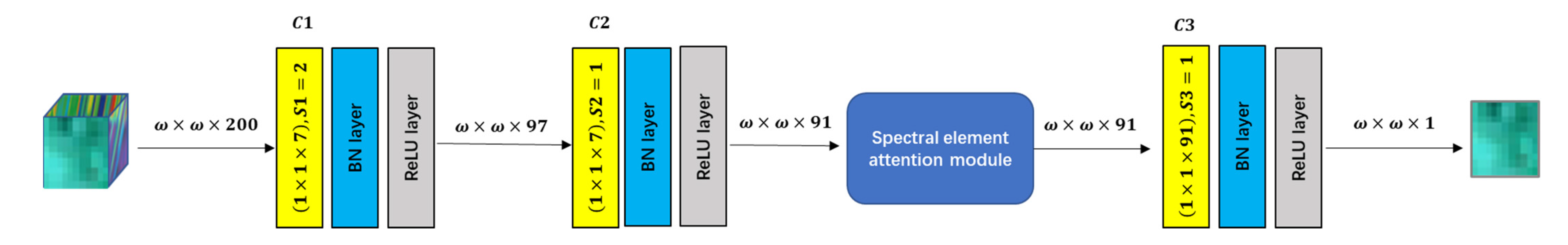
To express more clearly,

Table 1. The input, output, and parameters of convolutional operation for the Indian Pines data set.

Layer	Kernel Size	Stride	Input Shape	Output Shape
$C_1$	$1\times 1\times 7$	(1,1,2)	$7\times 7\times 200,1$	$7\times 7\times 97,24$
$C_2$	$1\times 1\times 7$	(1,1,1)	$7\times 7\times 97,24$	$7\times 7\times 91,24$
$C_{spe}$	$1\times 1\times 3$	(1,1,1)	$7\times 7\times 91,24$	$7\times 7\times 91,24$
$C_3$	$1\times 1\times 91$	(1,1,1)	$7\times 7\times 91,24$	$7\times 7\times 1,24$
$C_{spa}$	$3\times 3\times 1$	(1,1,1)	$7\times 7\times 1,24$	$7\times 7\times 1,24$

shows the shape of input data and output data and the specific parameters of the convolutional operation in the 3D-CSSEAN for the Indian Pines data set. The settings of Kennedy Space Center and Salinas Scene data sets are same as Indian Pines except for the band number of the input data. $C_{spe}$ and $C_{spa}$ in Table 1 indicate the convolution operation in the spectral element attention module and spatial element attention module, respectively. For each convolutional layer, $n^k$ were set to be 24 for each convolutional layer, and experiments show that the change of $n^k$ in a small range had little impact on the result.

4.2. Comparison and Analysis of Experimental Results

To evaluate the superiority and effectiveness of the proposed 3D-CSSEAN model, some machine learning and deep learning classification methods were compared with it. These methods included a traditional machine learning method SVM, state-of-the-art 3D deep learning models such as SSRN [20] and HybridSN [21], and the latest attention networks, such as CDSCN [28] and MAFN [32]. SVM was implemented by scikit-learn tools of the machine learning. The Radial Basis Function (RBF) was selected as the kernel function on the three data sets. The grid search method was used to determine the best values of parameters $C$ and $gamma$. Other comparison methods were implemented through code published in their papers [20,21,28,32]. For fairness of comparison, the input image patch size was set to $7\times 7\times B$ for all methods except HybridSN, where $B$ was the band number of the HSI. For HybridSN, in order to make the network work without changing the network structure, the input image patch size was set to $11\times 11\times B$, which was the closest parameter setting. For SVM and HybridSN, the number of PCA principal components was set to 30, which is the same as in the literature on HybridSN [21].

Classification results of the different methods on testing data of the three data set are reported in

Table 2. Classification results for Indian Pines data set. Bold represents the best results.

Class	SVM	HybridSN	SSRN	CDSCN	MAFN	3D-CSSEAN
1	100	89.01	90.00	89.82	96.53	100
2	58.08	87.41	93.77	94.24	95.22	96.24
3	73.78	86.04	88.60	94.89	93.15	96.66
4	89.81	89.56	92.28	91.40	90.74	94.79
5	96.70	95.69	97.40	98.83	97.50	98.41
6	98.31	96.75	97.73	98.39	98.97	97.92
7	90.00	96.31	50.00	98.38	83.69	94.39
8	93.24	92.42	96.85	97.78	99.36	99.75
9	80.00	78.81	30.00	98.75	97.95	98.57
10	70.79	87.32	90.83	94.33	94.49	96.35
11	71.34	90.72	94.89	95.03	98.28	98.25
12	61.91	89.28	94.11	91.15	93.84	97.38
13	100	94.55	99.73	98.81	96.89	98.07
14	93.54	94.62	97.11	97.51	99.29	98.33
15	89.72	93.16	94.58	92.49	95.09	94.66
16	99.17	90.49	98.34	97.90	92.53	94.30
AA	85.40 ± 3.12	90.76 ± 2.47	87.89 ± 6.48	95.61 ± 0.73	95.22 ± 1.16	97.13 ± 0.83
Kappa	73.65 ± 0.88	89.25 ± 1.23	93.40 ± 1.60	94.59 ± 1.06	95.99 ± 0.88	97.00 ± 0.65
OA	77.17 ± 0.74	90.60 ± 1.07	94.21 ± 1.41	95.26 ± 0.92	96.48 ± 0.78	97.37 ± 0.57

,

Table 3. Classification results for the Kennedy Space Center data set. Bold represents the best results.

Class	SVM	HybridSN	SSRN	CDSCN	MAFN	3D-CSSEAN
1	79.54	87.31	98.33	98.83	99.07	99.68
2	46.90	55.77	97.18	96.30	100	98.43
3	52.25	54.38	89.80	86.46	97.79	93.81
4	41.52	42.92	85.10	86.83	99.51	93.42
5	53.95	65.45	86.70	85.22	98.51	94.13
6	65.72	53.67	93.06	95.59	98.99	97.73
7	82.09	74.41	93.99	89.82	95.50	95.53
8	58.55	69.22	96.88	96.81	98.19	98.99
9	85.18	93.66	99.63	99.76	93.13	99.94
10	34.22	48.32	99.94	99.81	100	99.94
11	100	95.25	99.05	99.53	100	99.40
12	53.54	65.27	99.56	99.75	100	99.67
13	94.20	90.42	100	99.70	100	100
AA	65.21 ± 1.39	68.93 ± 2.75	95.34 ± 2.02	94.95 ± 1.19	98.02 ± 0.57	97.74 ± 0.99
Kappa	66.96 ± 1.19	71.48 ± 2.72	96.26 ± 1.63	96.54 ± 0.70	98.42 ± 0.38	98.48 ± 0.59
OA	70.43 ± 1.05	74.41 ± 2.45	96.64 ± 1.46	96.89 ± 0.62	98.60 ± 0.62	98.64 ± 0.53

and

Table 4. Classification results for the Salinas Scene data set. Bold represents the best results.

Class	SVM	HybridSN	SSRN	CDSCN	MAFN	3D-CSSEAN
1	100	99.95	100	99.97	99.92	99.98
2	99.66	99.74	99.87	99.91	99.94	99.79
3	100	99.87	99.59	98.73	99.5	98.49
4	99.84	99.05	99.20	99.46	97.04	99.28
5	97.99	96.11	99.42	99.05	98.87	99.42
6	100	99.84	99.98	99.91	99.53	99.97
7	99.78	99.72	99.99	99.95	99.85	99.84
8	83.92	93.90	92.84	90.42	97.23	97.33
9	99.62	99.50	99.86	99.73	99.71	99.79
10	99.30	98.36	99.39	97.87	98.49	99.31
11	99.98	98.70	97.60	97.67	97.36	97.27
12	99.39	99.07	99.04	99.33	99.16	99.74
13	97.18	97.5	99.49	99.56	95.86	98.86
14	99.78	94.51	97.29	97.28	98.61	98.44
15	88.59	90.68	93.87	87.57	93.22	94.40
16	99.64	98.96	100	99.98	98.76	99.99
AA	97.79 ± 0.22	97.84 ± 0.46	98.59 ± 0.14	97.9 ± 0.36	98.32 ± 0.28	98.87 ± 0.30
Kappa	93.94 ± 0.44	96.38 ± 0.54	97.08 ± 0.28	95.39 ± 0.83	97.7 ± 0.29	98.17 ± 0.34
OA	94.57 ± 0.39	96.75 ± 0.49	97.38 ± 0.25	95.86 ± 0.75	97.93 ± 0.26	98.35 ± 0.31

. As shown, 3D-CSSEAN achieved the best results on most indicators compared with the other methods. In our cases, the classification performances of all deep learning methods were better than those of SVM, which indicates that these deep learning models are generally superior to the traditional machine learning method in HSI classification. On the Indian Pines data set, the 3D-CSSEAN, MAFN, and CDSCN achieved better results than other methods. These results show that in the case of imbalanced categories, these attention models pay more attention to meaningful features, so they achieved better results. Compared with the two other attention methods, the 3D-CSSEAN increased the score at least 0.89%, 1.52%, and 1.01% in the OA, AA, and Kappa, respectively. Moreover, the AA of the 3D-CSSEAN was 0.89% higher than the best result of the other compared methods. These results indicate that the proposed method has good stability and robustness under the condition of unbalanced samples.

On the Kennedy Space Center data set, the 3D-CSSEAN, SSRN, CDSCN, and MAFN achieved at least 22% improvement compared to HybridSN and SVM. The reasons for this may be that HybridSN and SVM use PCA for dimension reduction, while the 3D-CSSEAN, SSRN, CDSCN, and MAFN are end-to-end network structures. The data dimension reduction module in the end-to-end is implemented in a supervised way, so the effect is better than the unsupervised way of PCA. Compared with SSRN and CDSCN, the 3D-CSSEAN achieved 2% and 1.75% improvement on OA, respectively. As for the latest MAFN, the 3D-CSSEAN also achieved comparable results. MAFN was slightly better than the 3D-CSSEAN on AA. The possible reason is that the spatial distribution of some categories in the Kennedy Space Center data set was relatively scattered. MAFN uses the correlation-based attention method to extract spatial features. Correlation-based methods may better capture the connections between scattered samples of these categories, so as to obtain more ideal results. The increase in accuracy of these categories can improve AA. On the Salinas Scene data set, all methods achieved higher than the 94% overall accuracy, while the 3D-CSSEAN was 0.42, 0.47, and 0.55 higher than the best result of the other methods on OA, Kappa, and AA, respectively.

In general, the three attention methods, CDSCN, MAFN and 3D-CSSEAN, achieved good results, indicating that the attention features extracted by them are beneficial to classification. These results indicated that the proposed element attention method can also effectively improve the classification performance. According to the results of the three data sets, the 3D-CSSEAN has good generalization ability on different data sets.

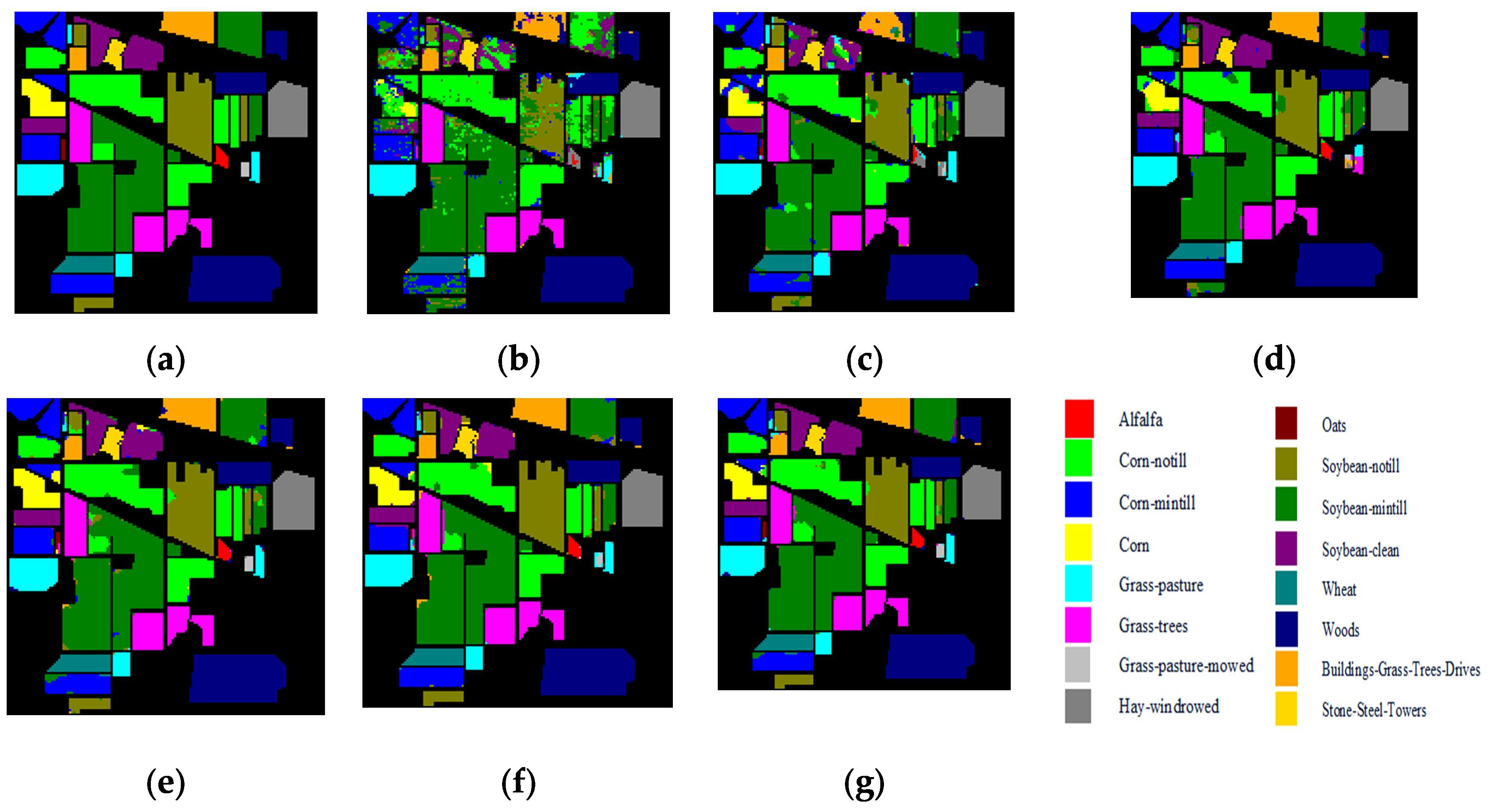
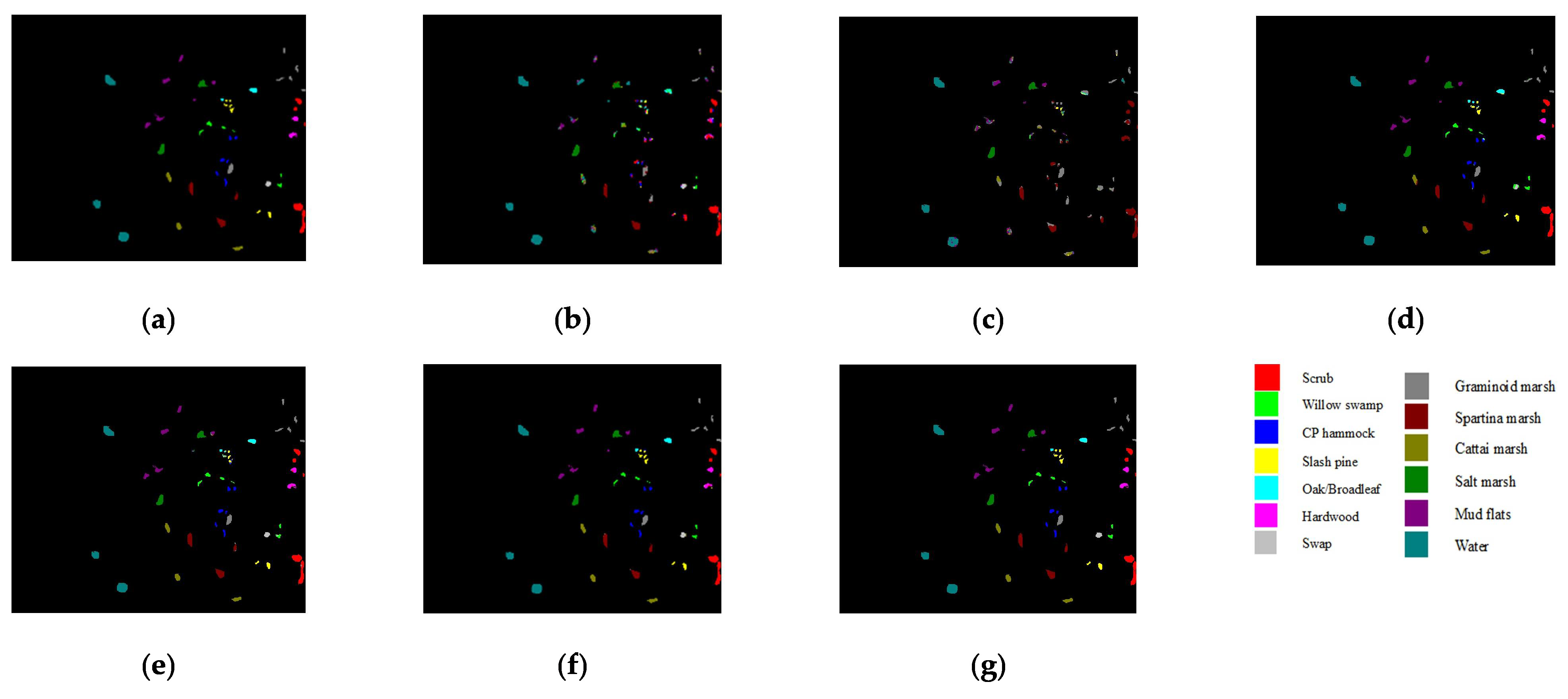
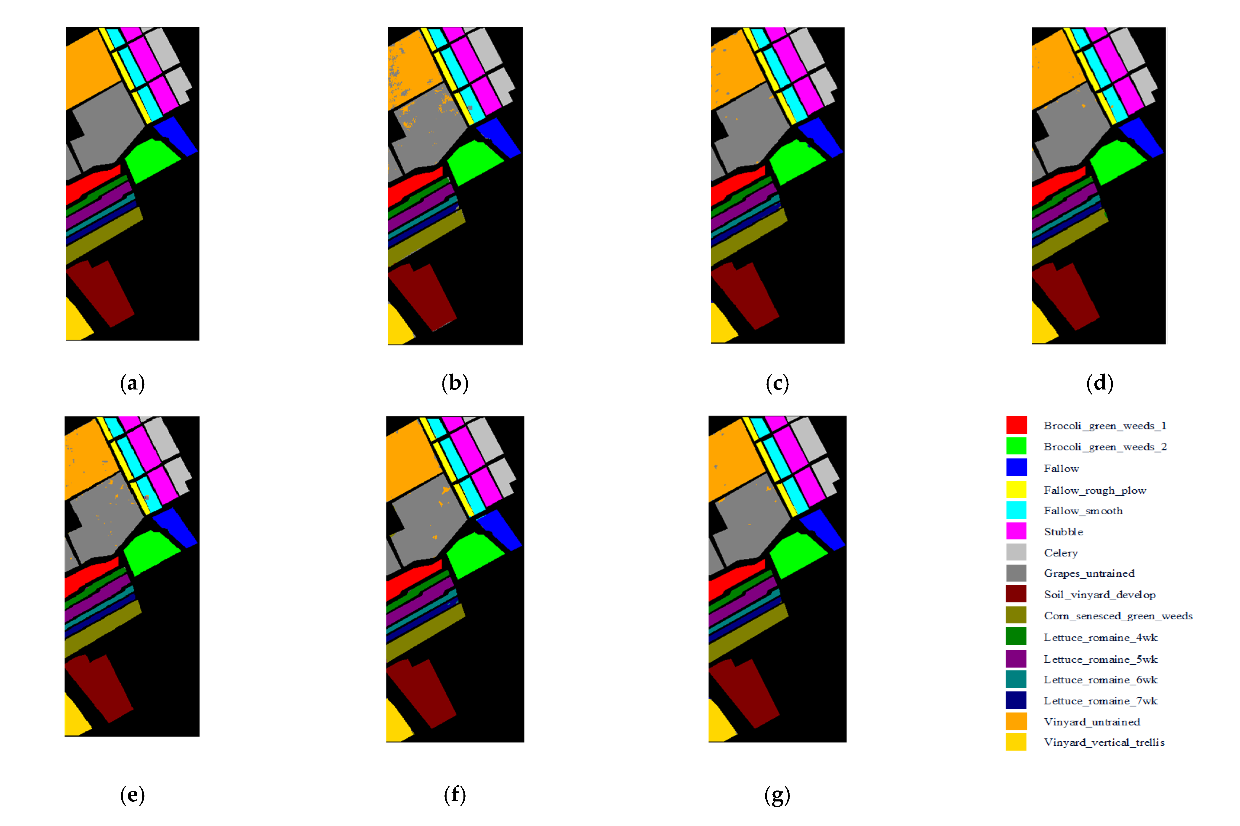
The classification maps of the five methods and the corresponding ground truth maps of the three data sets are shown in Figure 12, Figure 13 and Figure 14. It can be clearly seen from these results that the higher the classification accuracy, the better the continuity of the classification map. For the Indian Pines data set, there were obvious noise and discontinuous regions, as shown in Figure 12b, while the classification effect of the 3D-CSSEAN was relatively good. As shown in Figure 13, although there are very few labeled samples in the Kennedy Space Center data set, the 3D-CSSEAN still achieved good results. On the contrary, many obvious misclassified pixels can be seen in Figure 13b,c. All methods achieved over 94% overall accuracy on Salinas Scene data sets; however, there were still significant differences, which can be observed in Figure 14. It can be seen from Figure 14g that the 3D-CSSEAN still performed well at the edge of the category and the easily confused area.

Training and testing times provide a direct measure of the computational efficiency of HSI classification methods. In

Table 5. Training and testing times of different models for the three HSI data sets.

		Indian Pines	Kennedy Space Center	Salinas Scene
SVM	Train. (s)	0.10	0.74	0.80
	Test. (s)	1.34	6.30	37.55
HybridSN	Train. (s)	13.82	10.48	15.28
	Test. (s)	0.62	0.33	3.60
SSRN	Train. (s)	89.23	45.16	82.11
	Test. (s)	3.25	1.41	16.94
CDSCN	Train. (s)	114.47	61.49	121.19
	Test. (s)	4.36	2.04	25.15
MAFN	Train. (s)	374.62	264.07	389.35
	Test. (s)	10.38	5.41	88.43
3D-CSSEAN	Train. (s)	60.20	33.91	64.00
	Test. (s)	2.32	1.05	14.40

, the training time and the test time on the test data of different methods are shown. As presented in Table 5, because their inputs were the data under dimension reduction through PCA, the training time of SVM and HybridSN was significantly lower than that of other methods. Additionally, the time efficiency of the 3D-CSSEAN was higher than that of SSRN, CDSCN, and MAFN. As for MAFN, this may be because it uses a mixture of global operation-based and correlation-based methods to extract attention features, so it is relatively time-consuming. In particular, the training and testing time of the 3D-CSSEAN was about half that of the CDSCN method. The possible reason for this is that CDSCN adopts the dual branches mode, while the 3D-CSSEAN adopts the single branch mode, and thus it can save about half of the running time.

4.3. Ablation Studies

Three ablation experiments were conducted to analyze the contribution of different attention modules to HSI classification. The results are shown in

Table 6. OA (%) of the 3D-CSSEAN with different attention modules on the three data sets. Bold represents the best results.

Attention Module	Indian Pines	Kennedy Space Center	Salinas Scene
NONE	94.20 ± 0.83	94.98 ± 0.95	96.36 ± 0.98
SPE-EAN	96.01 ± 0.48	96.85 ± 0.80	97.16 ± 1.35
SPA-EAN	97.26 ± 0.69	97.72 ± 0.69	98.22 ± 0.31
3D-CSSEAN	97.37 ± 0.57	98.64 ± 0.53	98.35 ± 0.31

. NONE means the 3D-CSSEAN without spectral and spatial attention module. SPE-EAN indicates the 3D-CSSEAN only with the spectral attention module, and SPA-EAN indicates the 3D-CSSEAN only with the spatial attention module. The experimental results showed that any kind of attention module is helpful for classification. The role of the spatial attention module is more obvious than that of the spectral attention module. In terms of OA indicators, SPA-EAN increased 1.25%, 0.87%, and 1.06% more than SPE-EAN on Indian Pines, Kennedy Space Center, and Salinas Scene data sets, respectively. These results suggest that the spatial element attention module is more conducive to acquiring discriminative features for classification. The OA obtained by the 3D-CSSEAN had obvious improvement compared with the module without spectral–spatial attention. The OA of the 3D-CSSEAN was 3.17%, 3.66%, and 1.99% higher than without attention modules on Indian Pines, Kennedy Space Center, and Salinas Scene data sets, respectively. It can be seen from the results of ablation experiments that the proposed cascaded spectral–spatial element attention module can obtain more meaningful spectral and spatial features, thereby improving the final classification results.

To verify the contribution of $tanh$ activation function to the classification task, a series of experiments was conducted on the three data sets. Experiment results are shown in

Table 7. Experiment results of the 3D-CSSEAN without or with$tanh$ activate function on Indian Pines, Kennedy Space Center (KSC), and Salinas Scene data sets. Bold represents the best results.

Data Set	AA (without)	AA (with)	Kappa (without)	Kappa (with)	OA (without)	OA (with)
Indian Pines	96.64 ± 1.06	97.13 ± 0.83	96.36 ± 0.76	97.00 ± 0.65	96.81 ± 0.67	97.37 ± 0.57
KSC	96.92 ± 1.32	97.74 ± 0.99	97.93 ± 0.83	98.48 ± 0.59	98.15 ± 0.75	98.64 ± 0.53
Salinas Scene	98.83 ± 0.33	98.87 ± 0.30	98.03 ± 0.37	98.17 ± 0.34	98.23 ± 0.34	98.35 ± 0.31

. As can be seen from Table 7, AA, Kappa, and OA were all improved on the three data sets by using the $tanh$ function. Compared with the model without $tanh$, the OA score’s enhancements obtained by the 3D-CSSEAN with$tanh$ were 0.56% (Indian Pines), 0.49% (Kennedy Space Center), and 0.12% (Salinas Scene). The AA score’s increases were 0.49% (Indian Pines), 0.82% (Kennedy Space Center), and 0.04% (Salinas Scene). The Kappa coefficient’s improvements were 0.64% (Indian Pines), 0.55% (Kennedy Space Center), and 0.14% (Salinas Scene). These results indicate that the $tanh$ function is beneficial to enhance the separability of features and improve the classification performance. In addition, the standard deviation of all the results also decreased through using the$tanh$ function. This also shows that the stability of the model is improved by using the $tanh$ function.

5. Discussion

5.1. Influence of the Attention Block Number

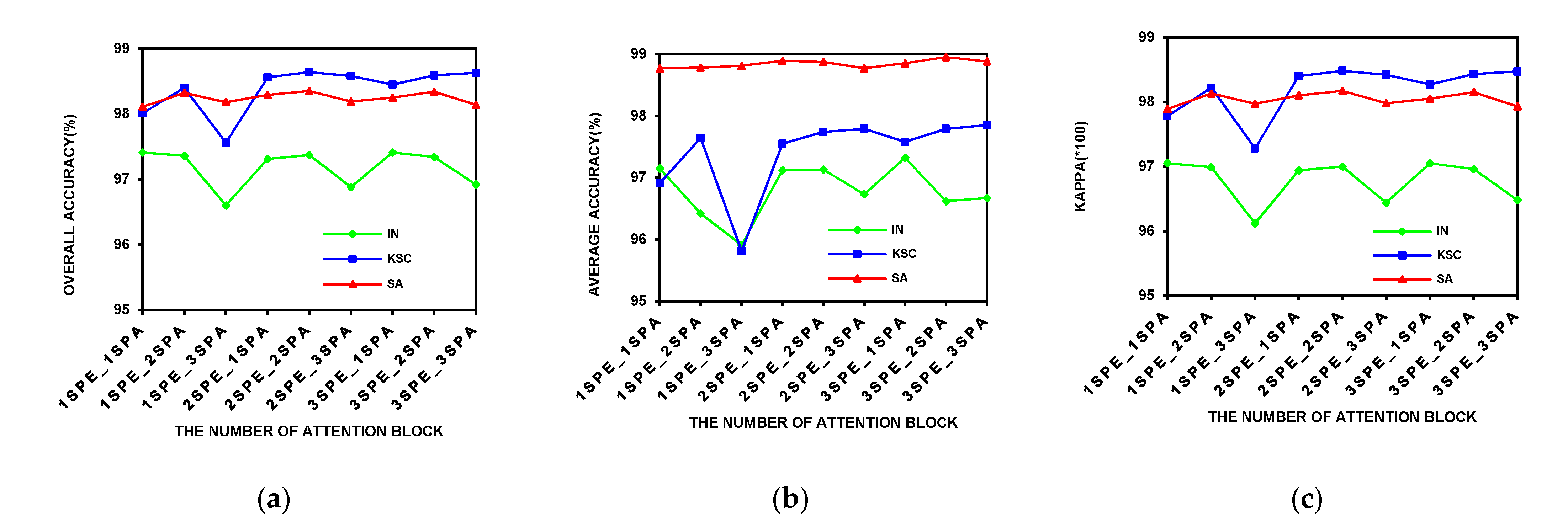
On three public data sets, the influence of the attention block number on the classification performance was analyzed. The experimental results are shown in Figure 15. In the figure, $iSPE\_jSPA$ of the horizontal axis represents $i$attention blocks in the spectral element attention module and $j$ attention blocks in the spatial element attention module. Figure 15a–c, respectively, show the influence of the attention block number on overall accuracy, average accuracy, and Kappa coefficient. As can be seen from the figure, on the Salinas Scene data set, the number of attention blocks had little effect on the results. Particularly, the model with $1SPE\_1SPA$ achieved good performance of OA at over 98%, indicating that the network structure with only one spectral element attention block cascading to one spatial element attention block extracted enough features for the improvement of the classification performance.

On the Indian Pines and Kennedy Space Center data sets, when the number of the spectral attention block was 1, three indicators all fluctuated greatly with the increase of spatial attention modules. In the case of $1SPE\_3SPA$, all the indicators were significantly reduced. This result shows that when the spectral features are not sufficiently extracted, blindly adding spatial depth features will not bring good results. When the spectral feature block was greater than 2, the indicators on the Kennedy Space Center data set tended to be stable, and at the same time, the fluctuation range on the Indian Pines data set was also narrowing.

When the number of spectral attention modules was 2, and the number of spatial attention modules was from 1 to 2, both OA and Kappa increased slightly on the three data sets. In the case of $2SPE\_2SPA$, the best OA was achieved on Kennedy Space Center and Salinas Scene data sets. As for the Indian Pines data set, when the number of attention module increased, the improvement in classification performance was limited. Furthermore, as the number of attention block increased, the time efficiency was bound to decrease. Overall, the network with $2SPE\_2SPA$ could achieve the best or very close to the best on three indicators. In addition, it had good performance on the three data sets, indicating that its generalization performance was better. Based on the above analysis, the network structure of our final model is $2SPE\_2SPA$.

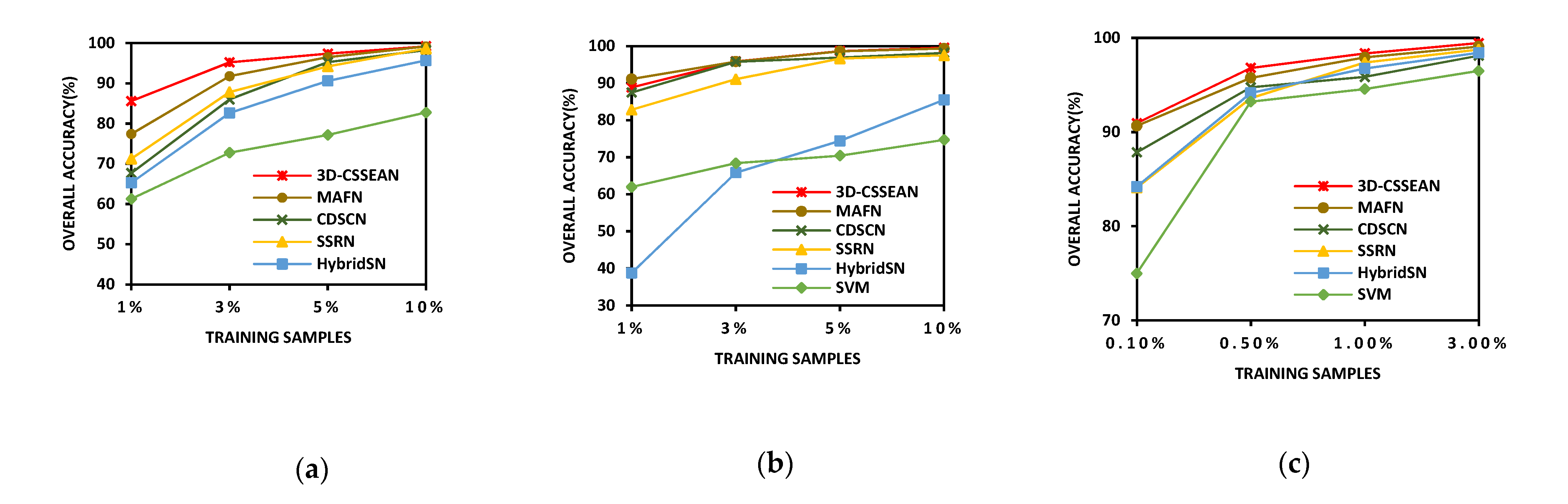
5.2. Influence of Different Training Sample Numbers

To evaluate the performance of the proposed 3D-CSSEAN, in this paper, under different numbers of training samples, four groups of labeled samples with different percentages were randomly selected as training samples for experiments. Specifically, 1%, 3%, 5%, and 10% of each category were randomly selected from the labeled samples as training samples on the Indian Pines data set and Kennedy Space Center data set, and 0.1%, 0.5%, 1%, and 3% of each category were randomly selected from the labeled samples as training samples on the Salinas Scene data set. The experiment results are shown in Figure 16.

On the Indian Pines data set, the advantages were more obvious when 1% and 3% of the labeled samples were used for training. Meaningful features extracted by the 3D-CSSEAN were more conducive to improving the classification performance in the case of small samples. Moreover, there was a significant decrease in the OA of CDSCN when only 3% of the labeled samples were used for training, indicating that CDSCN is prone to overfitting small training data. However, the 3D-CSSEAN did not increase many training parameters in the implementation of the attention module, and thus this problem can be avoided to some extent. On the Kennedy Space Center data set, the three different attention models, the 3D-CSSEAN, MAFN, and CDSCN, achieved better results than other methods, especially at 1% and 3%. These results indicate that these three attention features are beneficial for classification on the Kennedy Space Center data set. On the Salinas Scene data set, all methods achieved relatively close results, but the results of the 3D-CSSEAN were always the highest. In most cases, all methods could achieve good results, but in 0.10% of cases, the 3D-CSSEAN and MAFN had more obvious advantages.

In general, on Indian Pines and Salinas Scene data sets, the 3D-CSSEAN consistently outperformed the other approaches on all the training samples. As for the Kennedy Space Center data set, the results of the 3D-CSSEAN and MAFN were very close, and these results were better than those from the other comparison methods. Through these experimental investigations, it can be concluded that the 3D-CSSEAN has better classification performance and robustness in different training sample sets, and especially in the case of small samples, this advantage is more obvious. In addition, the MAFN method based on multiple attention combinations also demonstrated its competitiveness, especially on the Kennedy Space Center data set, where the spatial distribution of categories was relatively scattered. This shows that the combination of multiple attention methods is a promising research direction. In the future, perhaps the combination of the proposed element attention method and other attention methods will also produce more competitive results.

6. Conclusions

In this paper, a 3D cascaded spectral–spatial element attention network (3D-CSSEAN) is proposed to extract the meaningful features for hyperspectral image classification. The spectral element attention module and the spatial element attention module can make the network focus on primary spectral features and meaningful spatial features. Two element attention modules were implemented through several simple activation functions and elementwise multiplication. Therefore, the proposed model not only can obtain features that facilitate classification, but also has high computational efficiency. Since the implementation of the attention module does not add too many training parameters, it also makes the network structure suitable for small sample learning.

To evaluate the effectiveness of the method, extensive experiments were implemented on three public data sets: Indian Pines, Kennedy Space Center and Salinas Scene. Compared with the machine learning method, the popular deep learning methods and the attention methods, the proposed method obtained better classification performance. In cases with small samples, the advantages of the proposed method are more obvious. These results verify that the attention features obtained by the 3D-CSSEAN are beneficial for classification, and the 3D-CSSEAN is suitable for small sample learning. To evaluate the effectiveness of attention modules, several ablation experiments were conducted. From the results of the ablation experiments, both the spectral element attention module and the spatial element attention module have improved classification performance.

Extensive experiments showed that in the case of limited training samples, how to extract more meaningful features for classification is a direction worth exploring. In addition, the fusion of multiple attention features may be a kind of potential method, but how to ensure time efficiency may be a direction to be studied in the future.

References

1. Yang, X.G.; Yu, Y. Estimating Soil Salinity under Various Moisture Conditions: An Experimental Study. IEEE Trans. Geosci. Remote Sens. 2017, 55, 2525–2533. [Google Scholar] [CrossRef]
2. Peng, J.Y.; Yu, K.; Wang, J.; Zhang, Q.X.; Wang, L.; Fan, P. Mining painted cultural relic patterns based on principal component images selection and image fusion of hyperspectral images. J. Cult. Herit. 2019, 36, 32–39. [Google Scholar] [CrossRef]
3. He, L.; Li, J.; Liu, C.Y.; Li, S.T. Recent Advances on Spectral-Spatial Hyperspectral Image Classification: An Overview and New Guidelines. IEEE Trans. Geosci. Remote Sens. 2018, 56, 1579–1597. [Google Scholar] [CrossRef]
4. Melgani, F.; Bruzzone, L. Classification of hyperspectral remote sensing images with support vector machines. IEEE Trans. Geosci. Remote Sens. 2004, 42, 1778–1790. [Google Scholar] [CrossRef] [Green Version]
5. Zhang, E.L.; Zhang, X.R.; Liu, H.Y.; Jiao, L.C. Fast Multifeature Joint Sparse Representation for Hyperspectral Image Classification. IEEE Trans. Geosci. Remote Sens. 2015, 12, 1397–1401. [Google Scholar] [CrossRef]
6. Imani, M.; Ghassemian, H. An overview on spectral and spatial information fusion for hyperspectral image classification: Current trends and challenges. Inform. Fusion. 2020, 59, 59–83. [Google Scholar] [CrossRef]
7. Peng, J.T.; Jiang, X.; Chen, N.; Fu, H.J. Local adaptive joint sparse representation for hyperspectral image classification. Neurocomputing 2019, 334, 239–248. [Google Scholar] [CrossRef]
8. Kang, X.D.; Xiang, X.L.; Li, S.T.; Benediktsson, J.A. PCA-Based Edge-Preserving Features for Hyperspectral Image Classification. IEEE Trans. Geosci. Remote Sens. 2017, 55, 7140–7151. [Google Scholar] [CrossRef]
9. Li, Y.M.; Xie, T.J.; Wang, P.; Wang, J.; Liu, S.J.; Zhou, X.C.; Zhang, X.Z. Joint spectral-spatial hyperspectral image classification based on hierarchical subspace switch ensemble learning algorithm. Appl. Intell. 2018, 48, 4128–4148. [Google Scholar] [CrossRef]
10. Li, S.T.; Song, W.W.; Fang, L.Y.; Chen, Y.S.; Ghamisi, P.; Benediktsson, J.A. Deep Learning for Hyperspectral Image Classification: An Overview. IEEE Trans. Geosci. Remote Sens. 2019, 57, 6690–6709. [Google Scholar] [CrossRef] [Green Version]
11. Chen, Y.S.; Lin, Z.H.; Zhao, X.; Wang, G.; Gu, Y.F. Deep Learning-Based Classification of Hyperspectral Data. IEEE J.-Stars 2014, 7, 2094–2107. [Google Scholar] [CrossRef]
12. Zhang, X.R.; Liang, Y.J.; Li, C.; Ning, H.Y.; Jiao, L.C.; Zhou, H.Y. Recursive Autoencoders-Based Unsupervised Feature Learning for Hyperspectral Image Classification. IEEE Trans. Geosci. Remote Sens. 2017, 14, 1928–1932. [Google Scholar] [CrossRef] [Green Version]
13. Paoletti, M.E.; Haut, J.M.; Plaza, J.; Plaza, A. Scalable recurrent neural network for hyperspectral image classification. J. Supercomput. 2020, 76, 8866–8882. [Google Scholar] [CrossRef]
14. Shi, C.; Pun, C.M. Multiscale Superpixel-Based Hyperspectral Image Classification Using Recurrent Neural Networks With Stacked Autoencoders. IEEE Trans. Multimed. 2020, 22, 487–501. [Google Scholar] [CrossRef]
15. Yang, X.F.; Zhang, X.F.; Ye, Y.M.; Lau, R.Y.K.; Lu, S.J.; Li, X.T.; Huang, X.H. Synergistic 2D/3D Convolutional Neural Network for Hyperspectral Image Classification. Remote Sens. 2020, 12, 2033. [Google Scholar] [CrossRef]
16. Xu, H.; Yao, W.; Cheng, L.; Li, B. Multiple Spectral Resolution 3D Convolutional Neural Network for Hyperspectral Image Classification. Remote Sens. 2021, 13, 1248. [Google Scholar] [CrossRef]
17. Hu, W.; Huang, Y.Y.; Wei, L.; Zhang, F.; Li, H.C. Deep Convolutional Neural Networks for Hyperspectral Image Classification. J. Sens. 2015, 2015. [Google Scholar] [CrossRef] [Green Version]
18. Yang, X.F.; Ye, Y.M.; Li, X.T.; Lau, R.Y.K.; Zhang, X.F.; Huang, X.H. Hyperspectral Image Classification With Deep Learning Models. IEEE Trans. Geosci. Remote Sens. 2018, 56, 5408–5423. [Google Scholar] [CrossRef]
19. Ben Hamida, A.; Benoit, A.; Lambert, P.; Ben Amar, C. 3-D Deep Learning Approach for Remote Sensing Image Classification. IEEE Trans. Geosci. Remote Sens. 2018, 56, 4420–4434. [Google Scholar] [CrossRef] [Green Version]
20. Zhong, Z.L.; Li, J.; Luo, Z.M.; Chapman, M. Spectral-Spatial Residual Network for Hyperspectral Image Classification: A 3-D Deep Learning Framework. IEEE Trans. Geosci. Remote Sens. 2018, 56, 847–858. [Google Scholar] [CrossRef]
21. Roy, S.K.; Krishna, G.; Dubey, S.R.; Chaudhuri, B.B. HybridSN: Exploring 3-D-2-D CNN Feature Hierarchy for Hyperspectral Image Classification. IEEE Geosci. Remote Sens. Lett. 2020, 17, 277–281. [Google Scholar] [CrossRef] [Green Version]
22. Li, Z.W.; Cui, X.S.; Wang, L.Q.; Zhang, H.; Zhu, X.; Zhang, Y.J. Spectral and Spatial Global Context Attention for Hyperspectral Image Classification. Remote Sens. 2021, 13, 771. [Google Scholar] [CrossRef]
23. Qing, Y.H.; Liu, W.Y. Hyperspectral Image Classification Based on Multi-Scale Residual Network with Attention Mechanism. Remote Sens. 2021, 13, 335. [Google Scholar] [CrossRef]
24. Jie, H.; Li, S.; Gang, S. Squeeze-and-Excitation Networks. In Proceedings of the IEEE Conference on Computer Vision and Pattern Recognition (CVPR), Salt Lake City, UT, USA, 18–23 June 2018; pp. 7132–7141. [Google Scholar]
25. Woo, S.; Park, J.; Lee, J.Y.; Kweon, I.S. CBAM: Convolutional Block Attention Module. In Proceedings of the European Conference on Computer Vision (ECCV), Munich, Germany, 8–14 September 2018; p. 27. [Google Scholar]
26. Zhu, M.; Jiao, L.; Liu, F.; Yang, S.; Wang, J. Residual Spectral-Spatial Attention Network for Hyperspectral Image Classification. IEEE Trans. Geosci. Remote Sens. 2020, 59, 449–462. [Google Scholar] [CrossRef]
27. Tang, X.; Meng, F.; Zhang, X.; Cheung, Y.-M.; Ma, J.; Liu, F.; Jiao, L. Hyperspectral Image Classification Based on 3-D Octave Convolution With Spatial-Spectral Attention Network. IEEE Trans. Geosci. Remote Sens. 2020, 1–18. [Google Scholar] [CrossRef]
28. Cao, F.L.; Guo, W.H. Cascaded dual-scale crossover network for hyperspectral image classification. Knowl.-Based Syst. 2020, 189, 105122. [Google Scholar] [CrossRef]
29. Mou, L.C.; Zhu, X.X. Learning to Pay Attention on Spectral Domain: A Spectral Attention Module-Based Convolutional Network for Hyperspectral Image Classification. IEEE Trans. Geosci. Remote Sens. 2020, 58, 110–122. [Google Scholar] [CrossRef]
30. Sun, H.; Zheng, X.; Lu, X.; Wu, S. Spectral–Spatial Attention Network for Hyperspectral Image Classification. IEEE Trans. Geosci. Remote Sens. 2020, 58, 3232–3245. [Google Scholar] [CrossRef]
31. Haut, J.M.; Paoletti, M.E.; Plaza, J.; Plaza, A.; Li, J. Visual Attention-Driven Hyperspectral Image Classification. IEEE Trans. Geosci. Remote Sens. 2019, 57, 8065–8080. [Google Scholar] [CrossRef]
32. Li, Z.; Zhao, X.; Xu, Y.; Li, W.; Zhai, L.; Fang, Z.; Shi, X. Hyperspectral Image Classification with Multiattention Fusion Network. IEEE Geosci. Remote Sens. Lett. 2021, 1–5. [Google Scholar] [CrossRef]
Figure 1. The elemental attention mechanism used in the 3D-CSSEAN.
Remotesensing 13 02451 g001
Figure 2. The proposed framework of the 3D-CSSEAN.
Remotesensing 13 02451 g002
Figure 3. Global operation-based attention mechanism approaches for HSI classification: (a) schematic diagram of obtaining spectral attention features; (b) schematic diagram of obtaining spatial attention features. The symbol represents the dot multiplication.
Remotesensing 13 02451 g003
Figure 4. Correlation-based attention mechanism approach for HSI classification: (a) schematic diagram of obtaining spectral attention features; (b) schematic diagram of obtaining spatial attention features. The symbol   represents the matrix multiplication.
Remotesensing 13 02451 g004
Figure 5. Multifeature-based attention mechanism approach of the HSI. The symbol represents the element multiplication between features of two branches.
Remotesensing 13 02451 g005
Figure 6. Diagram of the data dimension reduction process on the Indian Pines data set.
Remotesensing 13 02451 g006
Figure 7. The attention module in the proposed 3D-CSSEAN.
Remotesensing 13 02451 g007
Figure 8. The spectral element attention block.
Remotesensing 13 02451 g008
Figure 9. The spatial element attention block.
Remotesensing 13 02451 g009
Figure 10. The curve of the tanh function.
Remotesensing 13 02451 g010
Figure 11. Comparison of visualization results before and after tanh function transformation: (a) the 100th band in the Salinas data set; (b) the 50th band in the Kennedy Space Center data set; (c) the 100th band in the Indian Pines data set; (df) represent the image after tanh transformation of (ac), respectively.
Remotesensing 13 02451 g011
Figure 12. Classification map for the Indian Pines data set: (a) ground truth; (b) SVM; (c) HybridSN; (d) SSRN; (e) CDSCN; (f) MAFN; (g) 3D-CSSEAN.
Remotesensing 13 02451 g012
Figure 13. Classification map for the Kennedy Space Center data set: (a) ground truth; (b) SVM; (c) HybridSN; (d) SSRN; (e) CDSCN; (f) MAFN; (g) 3D-CSSEAN.
Remotesensing 13 02451 g013
Figure 14. Classification map for the Salinas Scene data set: (a) ground truth; (b) SVM; (c) HybridSN; (d) SSRN; (e) CDSCN; (f) MAFN; (g) 3D-CSSEAN.
Remotesensing 13 02451 g014
Figure 15. Classification performance of the 3D-CSSEAN with different numbers of attention blocks. IN, KSC, and SA represent the Indian Pines, Kennedy Space Center, and Salinas Scene data sets, respectively. (a) Overall accuracy; (b) average accuracy; (c) Kappa coefficient.
Remotesensing 13 02451 g015
Figure 16. Overall accuracy (%) of the 3D-DSSEAN with different training sample proportions on the three data sets: (a) Indian Pines; (b) Kennedy Space Center; (c) Salinas Scene.
Remotesensing 13 02451 g016