Long-Term Analysis of Sea Ice Drift in the Western Ross Sea, Antarctica, at High and Low Spatial Resolution


Abstract
:
1. Introduction
2. Study Area and Data
2.1. ASAR High-Resolution Radar Image Data
2.2. NSIDC Sea Ice Motion Vector
3. Methods
3.1. Drift Vector Calculations
3.2. Validation of COSI-Corr Motion Vectors
3.3. Comparison Between High-Resolution and Low-Resolution Data
4. Results
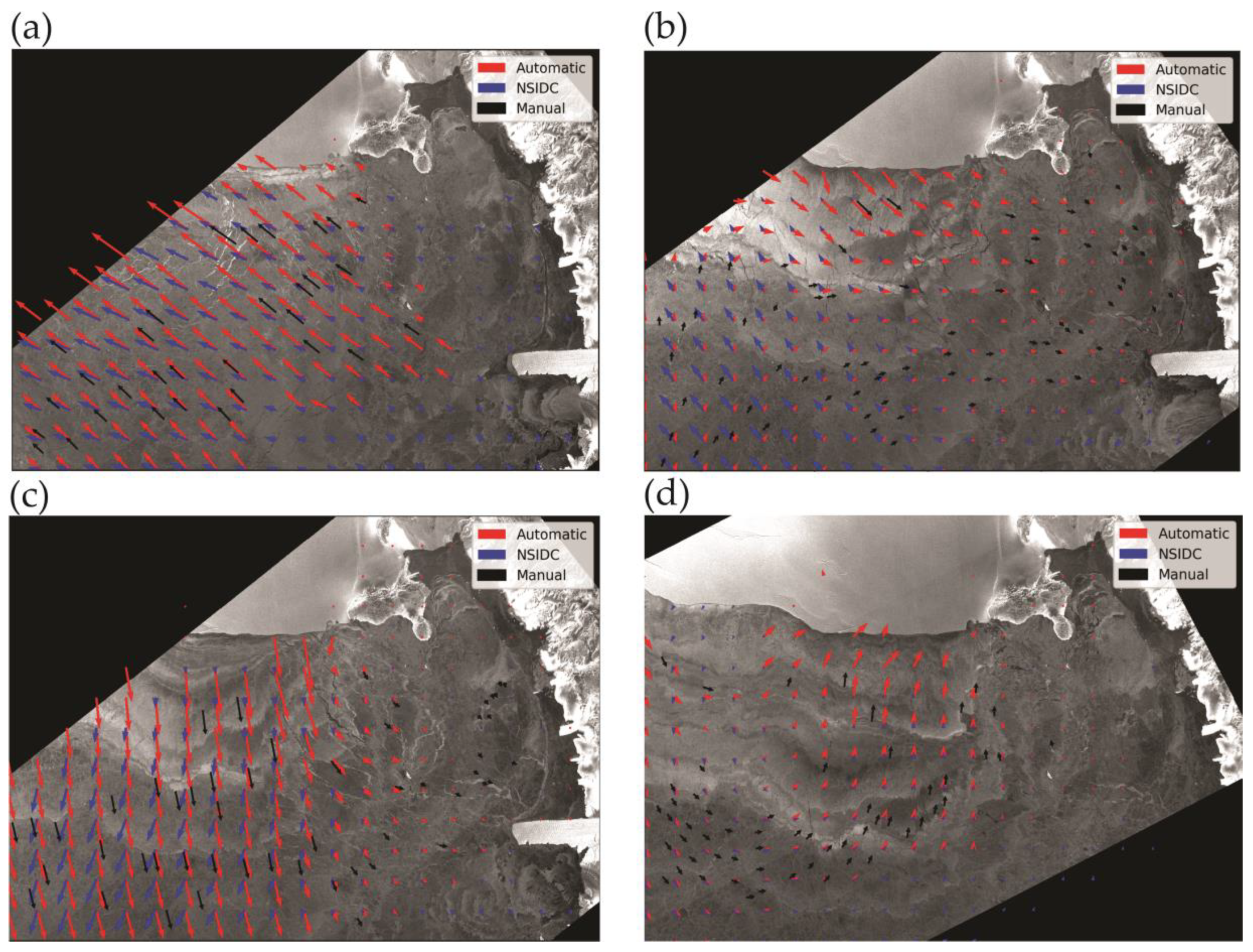
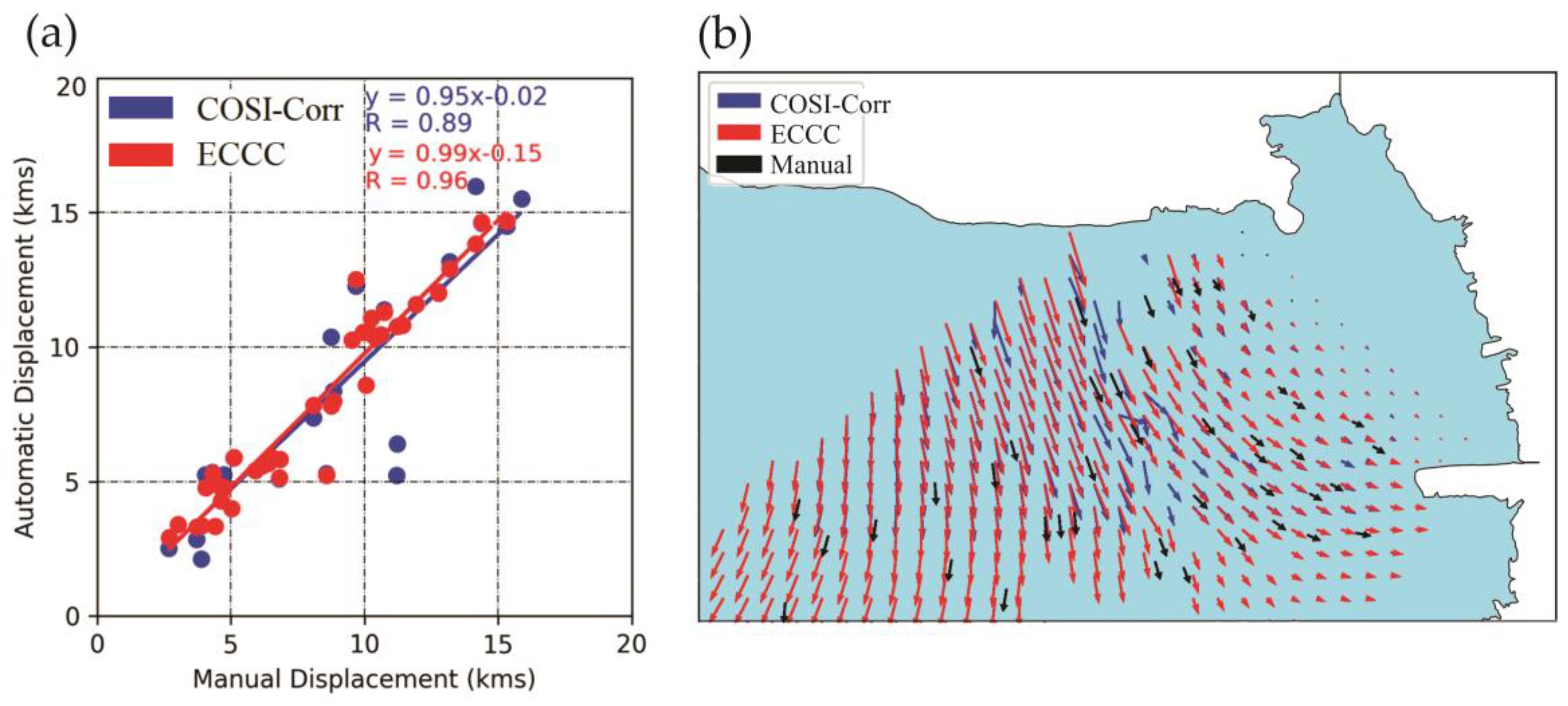
4.1. Validation Results: Envisat Manual Versus Automatic Vector
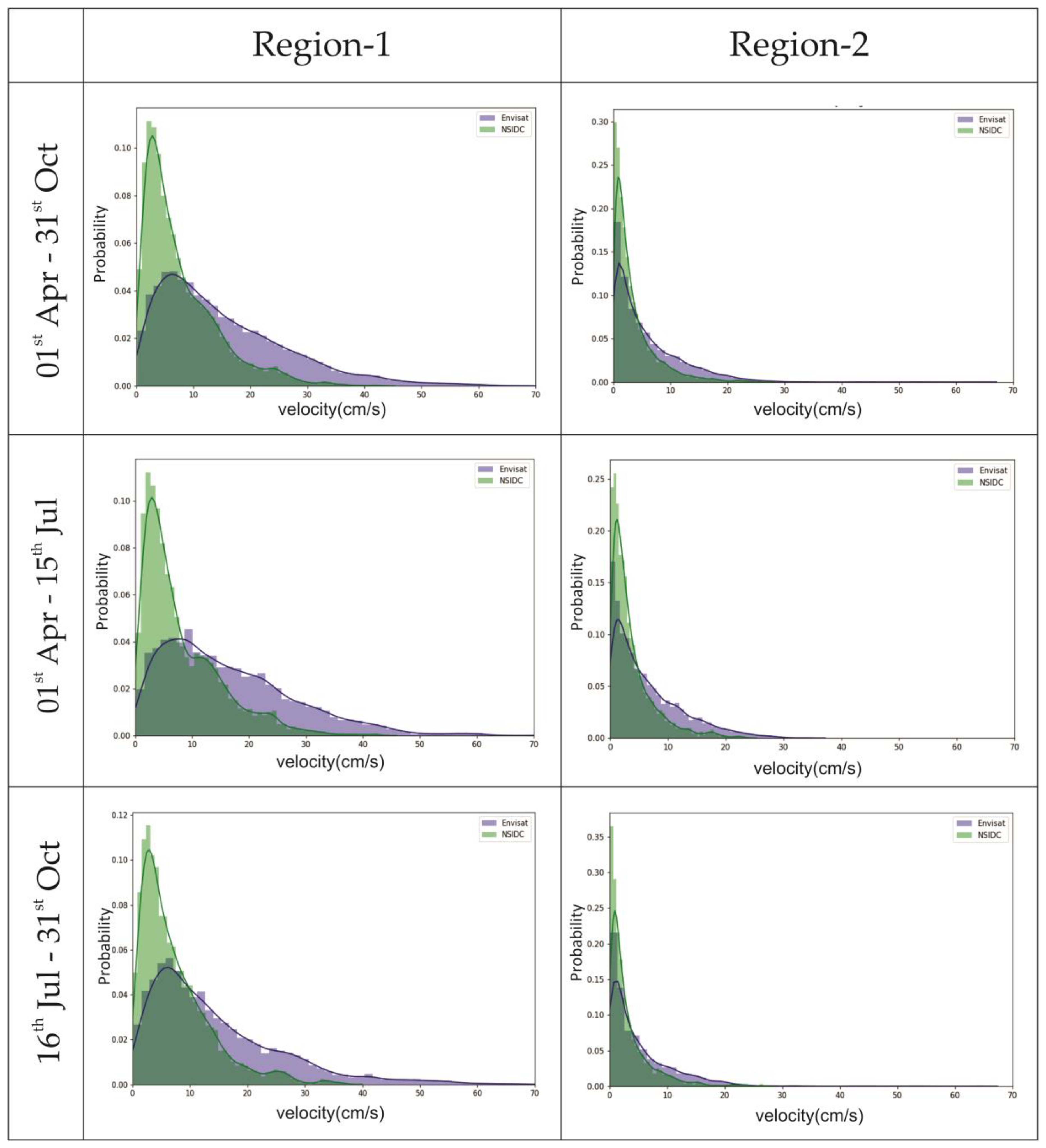
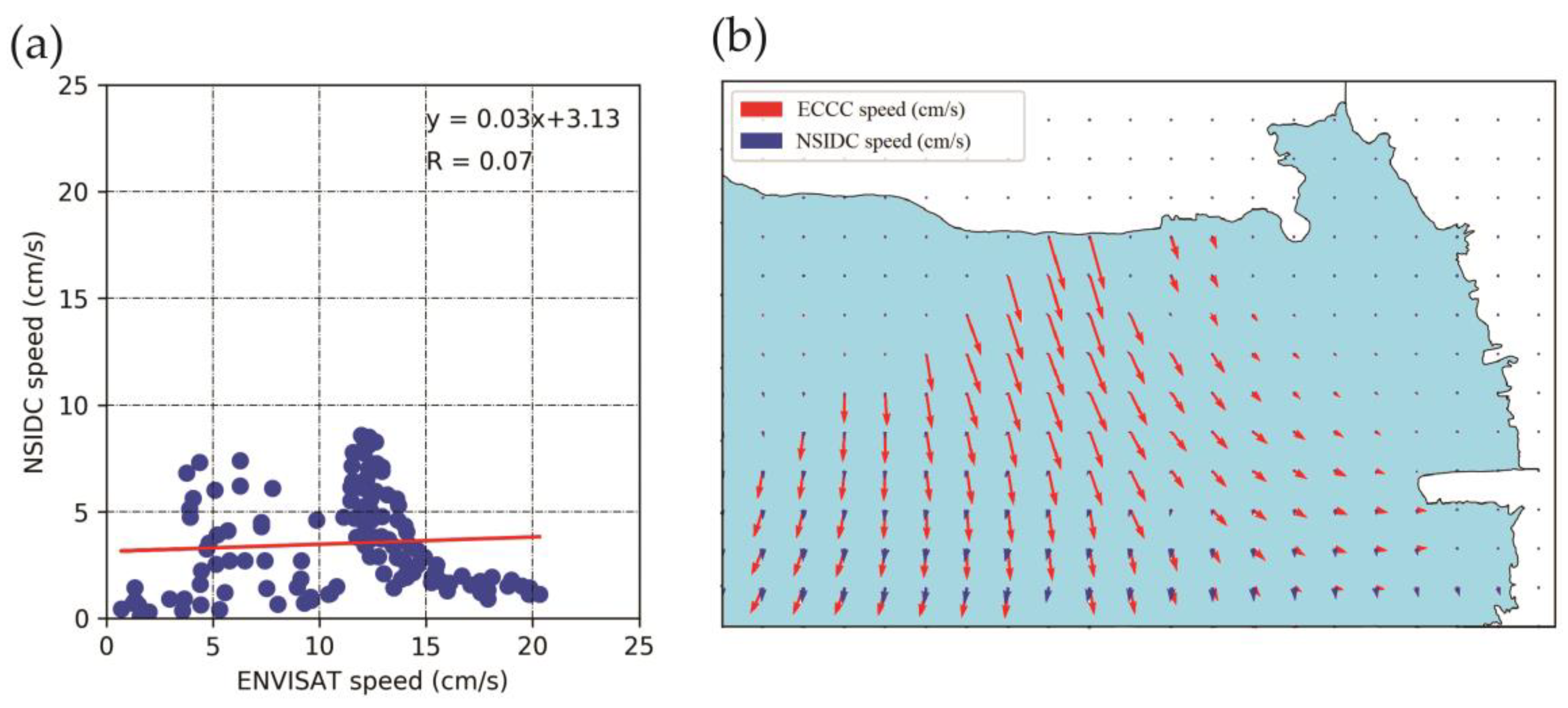
4.2. Envisat Automatic Versus NSIDC Vectors
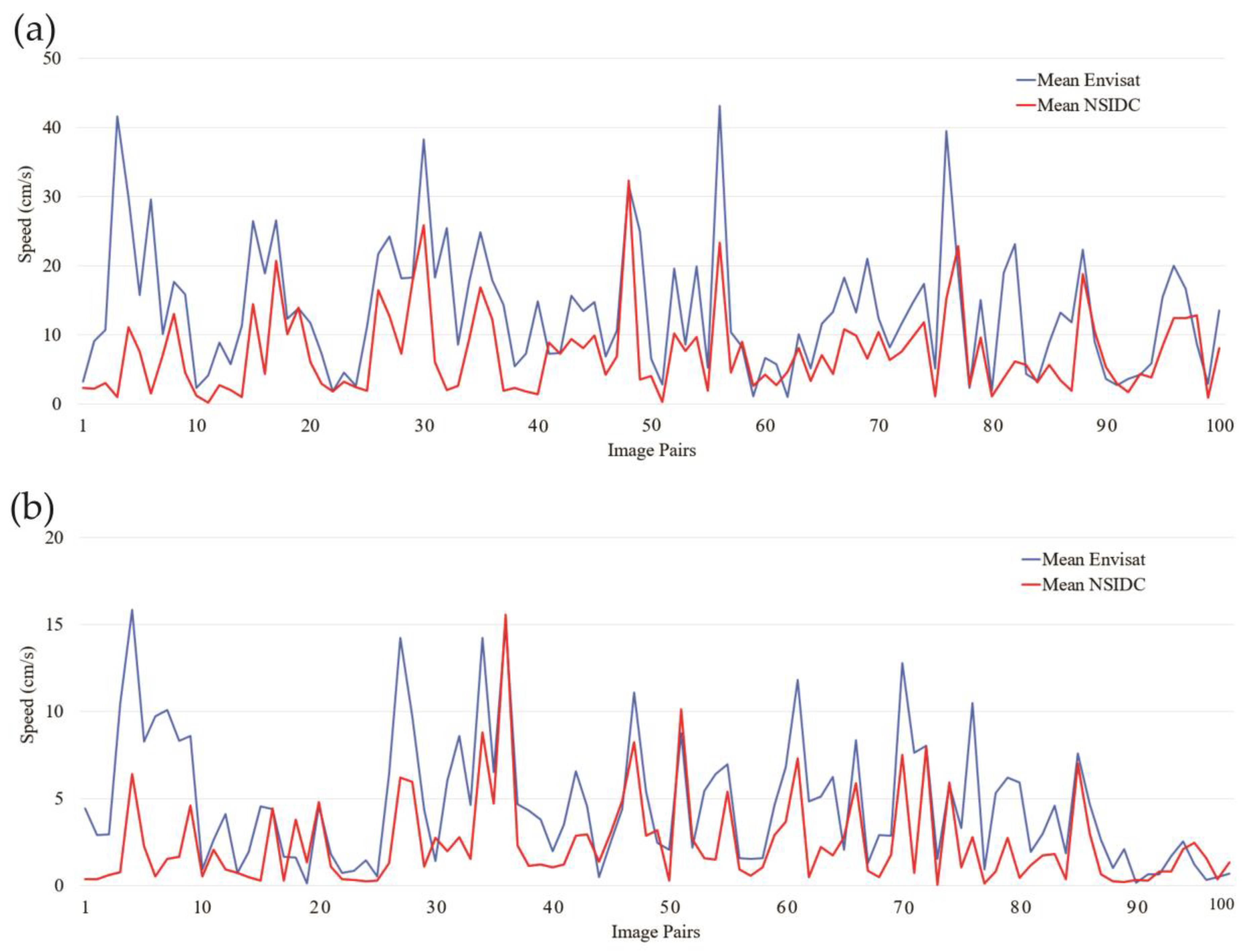
4.3. Average Speed Comparison Over the Study Area
5. Discussion
6. Conclusions
Author Contributions
Funding
Acknowledgments
Conflicts of Interest
References
- Bintanja, R.; Van Oldenborgh, G.; Drijfhout, S.; Wouters, B.; Katsman, C. Important role for ocean warming and increased ice-shelf melt in Antarctic sea-ice expansion. Nat. Geosci. 2013, 6, 376–379. [Google Scholar] [CrossRef]
- Haas, C. Dynamics versus thermodynamics: The sea ice thickness distribution. Sea Ice 2010, 82, 113–152. [Google Scholar]
- Leppäranta, M. The Drift of Sea Ice; Springer Science & Business Media: Heidelberg, Germany, 2011. [Google Scholar]
- Lindsay, R.; Zhang, J. The thinning of Arctic sea ice, 1988–2003: Have we passed a tipping point? J. Clim. 2005, 18, 4879–4894. [Google Scholar] [CrossRef]
- Parkinson, C.L. A 40-y record reveals gradual Antarctic sea ice increases followed by decreases at rates far exceeding the rates seen in the Arctic. Proc. Natl. Acad. Sci. USA 2019, 116, 14414–14423. [Google Scholar] [CrossRef] [Green Version]
- Maqueda, M.; Willmott, A.; Biggs, N. Polynya dynamics: A review of observations and modeling. Rev. Geophys. 2004, 42. [Google Scholar] [CrossRef] [Green Version]
- Dale, E.R.; McDonald, A.J.; Coggins, J.H.; Rack, W. Atmospheric forcing of sea ice anomalies in the Ross Sea polynya region. Cryosphere 2017, 11, 267–280. [Google Scholar] [CrossRef] [Green Version]
- Coggins, J.H.; McDonald, A.J. The influence of the Amundsen Sea Low on the winds in the Ross Sea and surroundings: Insights from a synoptic climatology. J. Geophys. Res. Atmos. 2015, 120, 2167–2189. [Google Scholar] [CrossRef]
- Kilifarska, N.; Bakhmutov, V.; Melnyk, G. Geomagnetic influence on Antarctic climate—Evidences and mechanism. Int. Rev. Phys. 2013, 7, 242–252. [Google Scholar]
- Haumann, F.A.; Gruber, N.; Münnich, M.; Frenger, I.; Kern, S. Sea-ice transport driving Southern Ocean salinity and its recent trends. Nature 2016, 537, 89–92. [Google Scholar] [CrossRef] [PubMed]
- Sun, Y. Automatic ice motion retrieval from ERS-1 SAR images using the optical flow method. Int. J. Remote Sens. 1996, 17, 2059–2087. [Google Scholar] [CrossRef]
- Petrou, Z.I.; Tian, Y. High-resolution sea ice motion estimation with optical flow using satellite spectroradiometer data. IEEE Trans. Geosci. Remote Sens. 2016, 55, 1339–1350. [Google Scholar] [CrossRef]
- Fily, M.; Rothrock, D. Sea ice tracking by nested correlations. IEEE Trans. Geosci. Remote Sens. 1987, GE-25, 570–580. [Google Scholar] [CrossRef]
- Hall, R.; Rothrock, D. Sea ice displacement from Seasat synthetic aperture radar. J. Geophys. Res. Oceans 1981, 86, 11078–11082. [Google Scholar] [CrossRef] [Green Version]
- Kwok, R. The RADARSAT geophysical processor system. In Analysis of SAR Data of the Polar Oceans; Springer: Berlin/Heidelberg, Germany, 1998; pp. 235–257. [Google Scholar]
- Kwok, R.; Curlander, J.C.; McConnell, R.; Pang, S.S. An ice-motion tracking system at the Alaska SAR facility. IEEE J. Ocean. Eng. 1990, 15, 44–54. [Google Scholar] [CrossRef]
- Thomas, M.; Geiger, C.; Kambhamettu, C. High resolution (400 m) motion characterization of sea ice using ERS-1 SAR imagery. Cold Reg. Sci. Technol. 2008, 52, 207–223. [Google Scholar] [CrossRef]
- Hollands, T.; Dierking, W. Performance of a multiscale correlation algorithm for the estimation of sea-ice drift from SAR images: Initial results. Ann. Glaciol. 2011, 52, 311–317. [Google Scholar] [CrossRef] [Green Version]
- Thomas, M.; Kambhamettu, C.; Geiger, C.A. Motion tracking of discontinuous sea ice. IEEE Trans. Geosci. Remote Sens. 2011, 49, 5064–5079. [Google Scholar] [CrossRef]
- Komarov, A.S.; Barber, D.G. Sea ice motion tracking from sequential dual-polarization RADARSAT-2 images. IEEE Trans. Geosci. Remote Sens. 2014, 52, 121–136. [Google Scholar] [CrossRef]
- Berg, A.; Eriksson, L.E. Investigation of a hybrid algorithm for sea ice drift measurements using synthetic aperture radar images. IEEE Trans. Geosci. Remote Sens. 2013, 52, 5023–5033. [Google Scholar] [CrossRef] [Green Version]
- Muckenhuber, S.; Korosov, A.A.; Sandven, S. Open-source feature-tracking algorithm for sea ice drift retrieval from Sentinel-1 SAR imagery. Cryosphere 2016, 10, 913–925. [Google Scholar] [CrossRef] [Green Version]
- Muckenhuber, S.; Sandven, S. Open-source sea ice drift algorithm for Sentinel-1 SAR imagery using a combination of feature tracking and pattern matching. Cryosphere 2017, 11, 1835. [Google Scholar] [CrossRef] [Green Version]
- Korosov, A.A.; Rampal, P. A Combination of Feature Tracking and Pattern Matching with Optimal Parametrization for Sea Ice Drift Retrieval from SAR Data. Remote Sens. 2017, 9, 258. [Google Scholar] [CrossRef] [Green Version]
- Giles, A.; Massom, R.; Heil, P.; Hyland, G. Semi-automated feature-tracking of East Antarctic sea ice from Envisat ASAR imagery. Remote Sens. Environ. 2011, 115, 2267–2276. [Google Scholar] [CrossRef]
- Tschudi, M.A.; Meier, W.N.; Stewart, J.S. An enhancement to sea ice motion and age products. Cryosphere Discuss 2019. [Google Scholar] [CrossRef] [Green Version]
- Sumata, H.; Lavergne, T.; Girard-Ardhuin, F.; Kimura, N.; Tschudi, M.A.; Kauker, F.; Karcher, M.; Gerdes, R. An intercomparison of A rctic ice drift products to deduce uncertainty estimates. J. Geophys. Res. Oceans 2014, 119, 4887–4921. [Google Scholar] [CrossRef] [Green Version]
- Hwang, B. Inter-comparison of satellite sea ice motion with drifting buoy data. Int. J. Remote Sens. 2013, 34, 8741–8763. [Google Scholar] [CrossRef]
- Sumata, H.; Kwok, R.; Gerdes, R.; Kauker, F.; Karcher, M. Uncertainty of Arctic summer ice drift assessed by high-resolution SAR data. J. Geophys. Res. Oceans 2015, 120, 5285–5301. [Google Scholar] [CrossRef] [Green Version]
- Sumata, H.; Gerdes, R.; Kauker, F.; Karcher, M. Empirical error functions for monthly mean Arctic sea-ice drift. J. Geophys. Res. Oceans 2015, 120, 7450–7475. [Google Scholar] [CrossRef]
- Szanyi, S.; Lukovich, J.V.; Barber, D.; Haller, G. Persistent artifacts in the NSIDC ice motion data set and their implications for analysis. Geophys. Res. Lett. 2016, 43, 10800–10807. [Google Scholar] [CrossRef]
- Heil, P.; Fowler, C.; Maslanik, J.; Emery, W.; Allison, I. A comparison of East Antarctic sea-ice motion derived using drifting buoys and remote sensing. Ann. Glaciol. 2001, 33, 139–144. [Google Scholar] [CrossRef] [Green Version]
- Schwegmann, S.; Haas, C.; Fowler, C.; Gerdes, R. A comparison of satellite-derived sea-ice motion with drifting-buoy data in the Weddell Sea, Antarctica. Ann. Glaciol. 2011, 52, 103–110. [Google Scholar] [CrossRef] [Green Version]
- Leprince, S.; Barbot, S.; Ayoub, F.; Avouac, J.-P. Automatic and precise orthorectification, coregistration, and subpixel correlation of satellite images, application to ground deformation measurements. IEEE Trans. Geosci. Remote Sens. 2007, 45, 1529–1558. [Google Scholar] [CrossRef] [Green Version]
- Envisat ASAR Product Handbook (Issue 2.2), Chapter 2: ASAR Products and Algorithms; European Space Agency: Paris, France, 2007.
- Scherler, D.; Leprince, S.; Strecker, M.R. Glacier-surface velocities in alpine terrain from optical satellite imagery—Accuracy improvement and quality assessment. Remote Sens. Environ. 2008, 112, 3806–3819. [Google Scholar] [CrossRef]
- Ayoub, F.; Leprince, S.; Keene, L. User’s Guide to COSI-CORR Co-Registration of Optically Sensed Images and Correlation; California Institute of Technology: Pasadena, CA, USA, 2009; p. 38. [Google Scholar]
- Howell, S.E.; Komarov, A.S.; Dabboor, M.; Montpetit, B.; Brady, M.; Scharien, R.K.; Mahmud, M.S.; Nandan, V.; Geldsetzer, T.; Yackel, J.J. Comparing L-and C-band synthetic aperture radar estimates of sea ice motion over different ice regimes. Remote Sens. Environ. 2018, 204, 380–391. [Google Scholar] [CrossRef]
- Howell, S.E.; Wohlleben, T.; Dabboor, M.; Derksen, C.; Komarov, A.; Pizzolato, L. Recent changes in the exchange of sea ice between the Arctic Ocean and the Canadian Arctic Archipelago. J. Geophys. Res. Oceans 2013, 118, 3595–3607. [Google Scholar] [CrossRef]
- Kwok, R. Satellite remote sensing of sea-ice thickness and kinematics: A review. J. Glaciol. 2010, 56, 1129–1140. [Google Scholar] [CrossRef] [Green Version]
- Hollands, T.; Dierking, W. Dynamics of the Terra Nova Bay Polynya: The potential of multi-sensor satellite observations. Remote Sens. Environ. 2016, 187, 30–48. [Google Scholar] [CrossRef] [Green Version]
- Hollands, T.; Linow, S.; Dierking, W. Reliability measures for sea ice motion retrieval from synthetic aperture radar images. IEEE J. Sel. Top. Appl. Earth Obs. Remote Sens. 2014, 8, 67–75. [Google Scholar] [CrossRef] [Green Version]
- Coggins, J.H.; McDonald, A.J.; Jolly, B. Synoptic climatology of the Ross Ice Shelf and Ross Sea region of Antarctica: K-means clustering and validation. Int. J. Climatol. 2014, 34, 2330–2348. [Google Scholar] [CrossRef]


| Months | 2002 | 2003 | 2004 | 2005 | 2006 | 2007 | 2008 | 2009 | 2010 | 2011 | 2012 |
|---|---|---|---|---|---|---|---|---|---|---|---|
| April | 8 | 8 | 18 | 16 | 14 | 6 | 11 | 12 | 27 | 5 | |
| May | 2 | 11 | 43 | 20 | 17 | 5 | 13 | 9 | 10 | ||
| June | 8 | 3 | 31 | 19 | 14 | 5 | 9 | 12 | 24 | ||
| July | 8 | - | 30 | 20 | 11 | 10 | 8 | 10 | 18 | ||
| August | 11 | 9 | 8 | 28 | 20 | 8 | 13 | 6 | 10 | 17 | |
| September | 8 | 10 | 16 | 31 | 9 | 6 | 11 | 4 | 7 | 17 | |
| October | 13 | 3 | 11 | 27 | 22 | 10 | 13 | 13 | 11 | 27 | |
| Annual Total | 32 | 48 | 57 | 208 | 126 | 80 | 63 | 64 | 71 | 140 | 5 |
| Grand Total | 894 | ||||||||||
| Displacement (km) | Directional Difference (deg) | |||||
|---|---|---|---|---|---|---|
| Algorithm | Slope | Intercept | R | RMSE | Image Pairs | |
| ECCC vs. manual | 1.00 ± 0.05 | −0.02 ± 0.38 | 0.98 ± 0.02 | 0.73 ± 0.41 | 24 | −0.79 ± 2.00 |
| COSI-Corr vs. manual | 1.05 ± 0.52 | −0.66 ± 2.10 | 0.92 ± 0.09 | 1.02 ± 0.82 | 24 | −3.17 ± 6.48 |
| COSI-Corr vs. ECCC | 0.77 ± 0.32 | 0.51 ± 3.05 | 0.84 ± 0.20 | 2.77 ± 3.86 | 894 | −0.04 ± 17.39 |
| (a) | Region-1—Speed (cm/s) | Image Pairs | Directional Difference (deg) | |||
| Year | Slope | Intercept | R | RMSE | ||
| 2002 | 0.07 ± 0.45 | 4.20 ± 4.75 | 0.30 ± 0.48 | 6.68 ± 4.97 | 22 | 3.57 ± 42.13 |
| 2003 | 0.18 ± 0.35 | 5.10 ± 4.58 | 0.27 ± 0.53 | 13.29 ± 9.68 | 27 | 9.75 ± 20.69 |
| 2004 | 0.09 ± 0.29 | 3.83 ± 3.60 | 0.09 ± 0.47 | 10.91 ± 9.12 | 27 | −9.61 ± 28.08 |
| 2005 | 0.15 ± 0.57 | 4.21 ± 7.79 | 0.20 ± 0.59 | 13.22 ± 10.75 | 101 | −9.34 ± 37.74 |
| 2006 | 0.06 ± 0.33 | 7.17 ± 6.78 | 0.06 ± 0.51 | 11.84 ± 10.19 | 92 | −1.38 ± 44.13 |
| 2007 | 0.09 ± 0.30 | 7.64 ± 6.83 | 0.14 ± 0.50 | 13.95 ± 10.41 | 40 | 5.11 ± 32.56 |
| 2008 | 0.13 ± 0.32 | 5.98 ± 5.69 | 0.19 ± 0.55 | 8.30 ± 7.26 | 23 | −3.59 ± 29.86 |
| 2009 | 0.16 ± 0.38 | 6.65 ± 8.62 | 0.23 ± 0.50 | 12.22 ± 9.65 | 25 | −6.52 ± 33.56 |
| 2010 | 0.27 ± 0.34 | 6.91 ± 7.32 | 0.33 ± 0.50 | 8.61 ± 5.87 | 16 | −0.43 ± 26.39 |
| 2011 | 0.20 ± 0.47 | 7.05 ± 11.62 | 0.22 ± 0.51 | 9.39 ± 8.37 | 104 | −2.18 ± 40.33 |
| 2012 | −0.13 ± 0.17 | 7.03 ± 3.49 | −0.20 ± 0.27 | 14.26 ± 5.15 | 4 | −15.03 ± 8.55 |
| Weighted Average | 0.13 | - | 0.18 | 11.33 | - | - |
| (b) | Region-2—Speed (cm/s) | Image Pairs | Directional Difference (deg) | |||
| Year | Slope | Intercept | R | RMSE | ||
| 2002 | 0.22 ± 0.32 | 2.18 ± 3.88 | 0.41 ± 0.44 | 3.58 ± 3.06 | 22 | −2.10 ± 47.65 |
| 2003 | 0.21 ± 0.23 | 2.04 ± 1.71 | 0.41 ± 0.48 | 4.10 ± 2.97 | 27 | −3.34 ± 43.90 |
| 2004 | 0.13 ± 0.19 | 1.67 ± 1.86 | 0.37 ± 0.41 | 4.60 ± 4.04 | 27 | −3.50 ± 54.06 |
| 2005 | 0.11 ± 0.30 | 2.91 ± 3.68 | 0.35 ± 0.42 | 6.32 ± 4.55 | 101 | −9.52 ± 39.85 |
| 2006 | 0.23 ± 0.28 | 3.00 ± 3.75 | 0.45 ± 0.43 | 4.96 ± 3.18 | 92 | 4.92 ± 38.99 |
| 2007 | 0.12 ± 0.18 | 4.28 ± 3.98 | 0.32 ± 0.38 | 5.83 ± 3.52 | 40 | 11.30 ± 50.01 |
| 2008 | 0.29 ± 0.51 | 2.46 ± 3.25 | 0.48 ± 0.39 | 3.99 ± 2.80 | 23 | 14.48 ± 42.00 |
| 2009 | 0.21 ± 0.26 | 3.59 ± 4.79 | 0.41 ± 0.35 | 5.19 ± 4.12 | 25 | −2.18 ± 56.15 |
| 2010 | 0.18 ± 0.12 | 2.50 ± 1.84 | 0.45 ± 0.27 | 5.55 ± 2.01 | 16 | 4.48 ± 31.61 |
| 2011 | 0.22 ± 0.43 | 2.96 ± 3.72 | 0.33 ± 0.41 | 4.72 ± 3.26 | 104 | 2.47 ± 45.92 |
| 2012 | 0.04 ± 0.07 | 1.78 ± 0.80 | 0.18 ± 0.51 | 11.84 ± 1.85 | 4 | −7.74 ± 3.13 |
| Weighted Average | 0.18 | - | 0.38 | 5.18 | - | - |
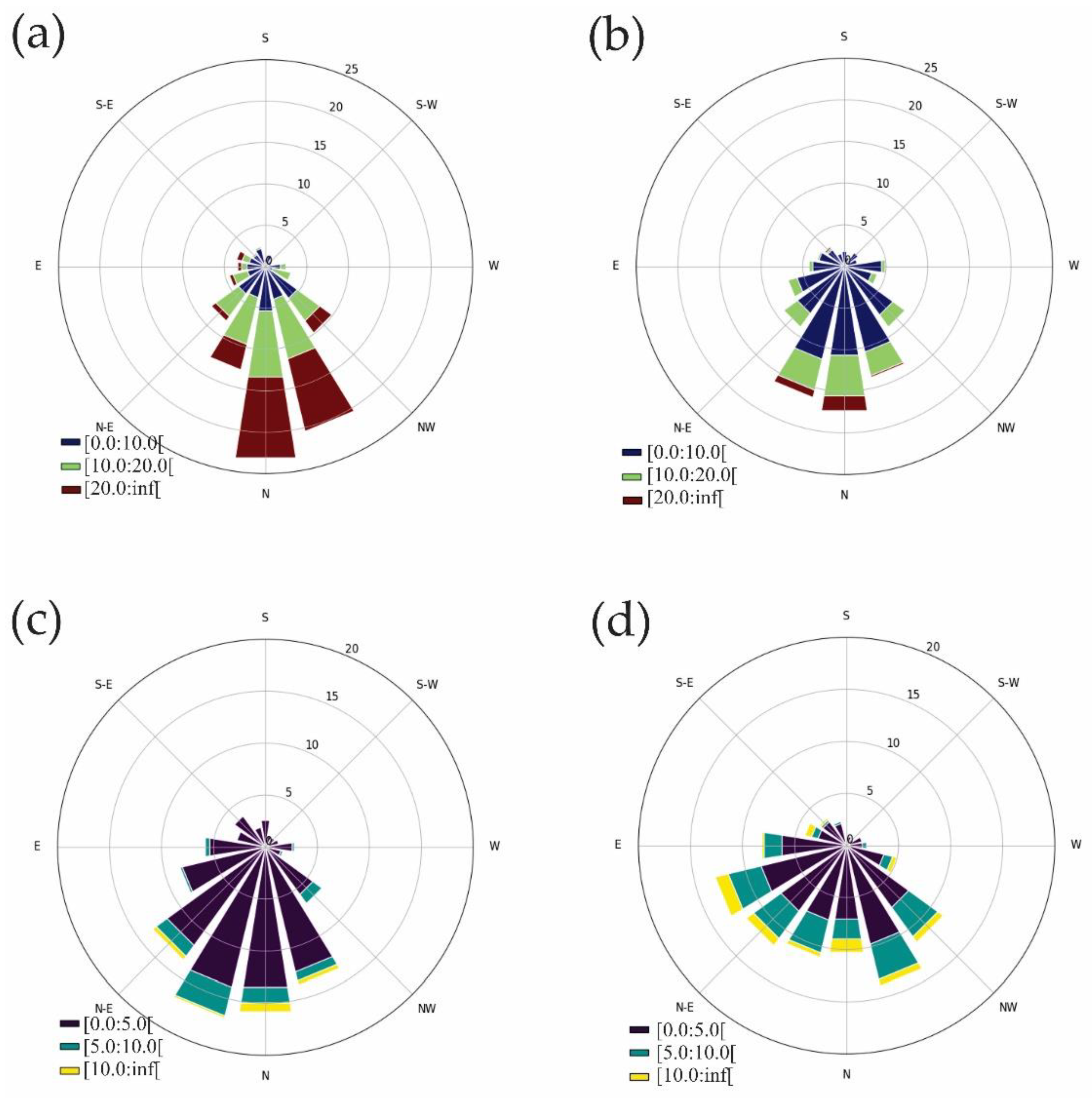
| (a) | Envisat (Region-1) | |||
| Categories (cm/s) | Low (0–10) | Medium (10–20) | High (>20) | |
| S | 6.07 | 0.22 | 0 | 6.29 |
| W | 6.07 | 5.17 | 0.45 | 11.7 |
| N | 17.3 | 24.27 | 24.04 | 65.6 |
| E | 9.66 | 5.17 | 1.57 | 16.4 |
| 39.1 | 34.83 | 26.07 | 100 | |
| (b) | NSIDC (Region-1) | |||
| Categories (cm/s) | Low (0–10) | Medium (10–20) | High (>20) | |
| S | 7.42 | 0 | 0 | 7.42 |
| W | 14.61 | 1.8 | 0 | 16.4 |
| N | 39.78 | 14.38 | 2.92 | 57.1 |
| E | 16.4 | 2.47 | 0.22 | 19.1 |
| 78.2 | 18.65 | 3.15 | 100 | |
| (c) | Envisat (Region-2) | |||
| Categories (cm/s) | Low (0–5) | Medium (5–10) | High (>10) | |
| S | 5.19 | 0.22 | 0 | 5.41 |
| W | 10.82 | 2.6 | 0.87 | 14.3 |
| N | 30.95 | 11.9 | 3.03 | 45.9 |
| E | 23.59 | 8.01 | 2.81 | 34.4 |
| 70.56 | 22.73 | 6.71 | 100 | |
| (d) | NSIDC (Region-2) | |||
| Categories (cm/s) | Low (0–5) | Medium (5–10) | High (>10) | |
| S | 7.36 | 0 | 0 | 7.36 |
| W | 8.23 | 1.08 | 0 | 9.31 |
| N | 49.13 | 6.49 | 1.95 | 57.6 |
| E | 24.68 | 1.08 | 0 | 25.8 |
| 89.39 | 8.66 | 1.95 | 100 | |
© 2020 by the authors. Licensee MDPI, Basel, Switzerland. This article is an open access article distributed under the terms and conditions of the Creative Commons Attribution (CC BY) license (http://creativecommons.org/licenses/by/4.0/).
Share and Cite
Farooq, U.; Rack, W.; McDonald, A.; Howell, S. Long-Term Analysis of Sea Ice Drift in the Western Ross Sea, Antarctica, at High and Low Spatial Resolution. Remote Sens. 2020, 12, 1402. https://doi.org/10.3390/rs12091402
Farooq U, Rack W, McDonald A, Howell S. Long-Term Analysis of Sea Ice Drift in the Western Ross Sea, Antarctica, at High and Low Spatial Resolution. Remote Sensing. 2020; 12(9):1402. https://doi.org/10.3390/rs12091402
Chicago/Turabian StyleFarooq, Usama, Wolfgang Rack, Adrian McDonald, and Stephen Howell. 2020. "Long-Term Analysis of Sea Ice Drift in the Western Ross Sea, Antarctica, at High and Low Spatial Resolution" Remote Sensing 12, no. 9: 1402. https://doi.org/10.3390/rs12091402