Evaluating Landfast Sea Ice Ridging near UtqiaġVik Alaska Using TanDEM-X Interferometry

Abstract

Seasonal landfast sea ice stretches along most Arctic coastlines and serves as a platform for community travel and subsistence, industry operations, and as a habitat for marine mammals. Landfast ice can feature smooth ice and areas of m-scale roughness in the form of pressure ridges. Such ridges can significantly hamper trafficability, but if grounded can also serve to stabilize the shoreward ice. We investigate the use of synthetic aperture radar interferometry (InSAR) to assess the formation and movement of ridges in the landfast sea ice near Utqiaġvik, Alaska. The evaluation is based on the InSAR-derived surface elevation change between two TanDEM-X bistatic image pairs acquired during January 2012. We compare the results with backscatter intensity, coastal radar data, and SAR-derived ice drift and evaluate the utility of this approach and its relevance for evaluation of ridge properties, as well as landfast sea ice evolution, dynamics, and stability.

1. Introduction

Landfast sea ice is a key component of many coastal Arctic ecosystems and provides essential services to marine biota and people [1]. Landfast ice serves as a habitat for marine mammals, such as seals and polar bears, and is routinely used for over-ice travel by coastal residents and industry [2]. Landfast ice also acts as a barrier, protecting the shore from winter storms and erosion in many areas [3,4]. On the other hand, landfast ice can also block or result in hazardous conditions for marine traffic [1,5].

Landfast ice can either form through in-situ freezing or by pack ice drifting into place. It can remain in place for weeks to months during winter anchored to the sea floor through ridges or by coastal morphology preventing the ice from moving during offshore winds or currents. The extent of landfast ice depends on bathymetry, as well as ice, ocean, and atmospheric conditions, and varies substantially with region. In the Laptev, Kara, and East Siberian seas, landfast ice can extend over one hundred kilometers offshore, in part due to the predominate offshore wind environment resulting in little strain from interaction with the pack ice [6,7,8,9].

In the Beaufort and Chukchi seas, landfast ice is typically narrower than in the Russian Arctic and ranges from a few to several tens of kilometers [10]. Here, landfast ice is more extensive with longer duration in the eastern Beaufort Sea than in the Chukchi Sea. This is largely due to the coastal morphology in relation to the Beaufort Gyre which creates a dynamic sea ice environment in the western Beaufort and Chukchi seas [8]. Utqiaġvik, Alaska, previously known as Barrow, is situated near point Barrow, the confluence between the Beaufort and the Chukchi Seas. Here, the landfast ice season lasts from late fall or early winter to late spring [10,11]. During this time the landfast ice is used as a platform for subsistence activities by local residents, including hunting of bowhead whales, beluga, and seals [12,13,14,15,16].

Landfast sea ice stability refers to the ability for the ice to remain in place during wind and current events. Stability plays a vital role for landfast ice users and for marine traffic due to the potential hazard of break-out events. The stability throughout the season is determined by many factors, including ice thickness, coastal morphology, and anchoring points such as islands and grounded pressure ridges [8]. Significant work has gone into understanding the stability of the landfast ice cover near Utqiaġvik in the context of the frictional force from grounded ridges [8,16,17]. Besides resulting in stable anchoring points, ridges and the ice surface morphology can hamper the use of parts of the coastal ice by inhibiting transportation. Therefore, ample studies have contributed to the understanding of landfast ice dynamics [18], ridge formation [8,11], and how ridges impact trafficability of the ice [19,20,21]. Through such work, ridge height has been measured using ground-based electromagnetic conductivity [21], helicopter-borne laser profilers [22], airborne laser scanners [23], structure-from-motion [20], and spaceborne altimeters [24].

Sea ice topography can also be evaluated through synthetic aperture radar interferometry (InSAR) [25]. InSAR is a technique that utilizes the phase component of complex SAR scenes. The phase difference between two scenes is related to the topography or the motion of the ice [26,27,28]. Hence, for stable landfast ice, the phase difference is nearly directly proportional to ice topography if the scenes are acquired within roughly one second [26,29]. With larger temporal baselines on the order of seconds, the phase signal can be significantly impacted by vertical motion due to ocean waves [30]. TanDEM-X is a SAR constellation that allows for bistatic acquisition of images with temporal baselines in the order of milliseconds. This data has been used to assess the surface morphology and height of grounded ridges in the landfast ice near Utqiaġvik [20,31], sea ice in the Fram Strait [32,33], and icebergs in the Southern Sea [34].

The previous studies mentioned have demonstrated the value of InSAR for assessment of ice ridges. However, to our knowledge, this technique has not previously been used to evaluate their formation and displacement. Here, we present a change detection approach based on bistatic X-band InSAR to detect the evolution of ridges. We apply this approach to the landfast sea ice near Utqiaġvik and validate the results using backscatter–intensity features, coastal radar data, and SAR-derived sea ice drift [35]. In this effort, we investigate InSAR as a tool to capture ridging events which can help provide insight into relevant properties and processes within the landfast ice critical to ice stability and use.

2. Data

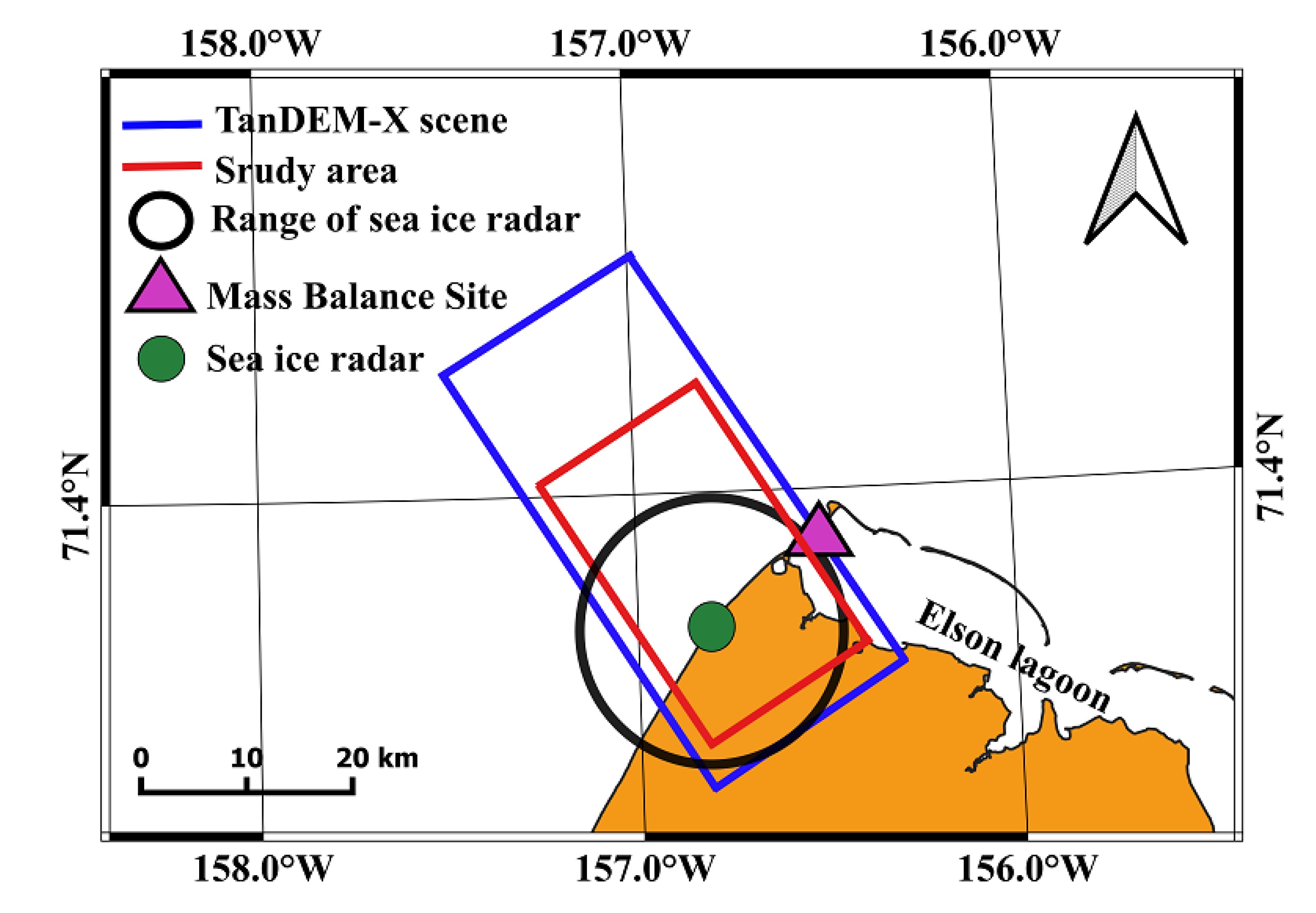
2.1. Study Site and Local Data and Conditions

The focus of this study is the landfast ice near Utqiaġvik, Alaska (Figure 1). Here, the near-shore ice is monitored every ~5 min with a Furuno FAR-2127 25 kW, X-band (3 cm, 10 GHz) marine radar from an altitude of 22.5 m [36]. The nominal range of the radar is 10 km (shown in Figure 1). Factors that determine what can be detected include the size and orientation of the scattering objects, atmospheric conditions, ocean conditions, ridge sizes, and ice properties. Features can also be occluded, or in the shadow of, other features closer to the radar [8,37,38]. It is not possible to estimate ridge height with the Utqiaġvik radar system because the intensity of the backscatter signal depends on the factors mentioned above, and can vary as these conditions vary [16]. The landfast ice is clearly visible in the radar images, with ridges appearing as bright linear features (Figure 2). The values in the radar imagery have no physical units due to the nature of the signal processing by the radar system. The 8-bit pixel values are stretched between 0 and 255. Rough ice areas on the ocean, and buildings, fences, and cars on land also return strong signals. Dark regions may indicate open water or smooth ice or shadow zones behind large ridges [8,16,39]. The radar images are used for monitoring landfast ice and provide information about the dynamics of drifting ice [39] and deformation events [8].

We identified a number of ridging events using coastal radar data during 2006–2016 through visual interpretation of large changes in the backscatter. We chose to focus on a time period between 13 and 24 Jan 2012 based on access to TanDEM-X data and the occurrence of ridging. Several events took place during this time due to onshore convergence resulting in both the development of new ridges as well as displacement of existing ones, which are visible in the radar imagery (e.g., red arrows in Figure 2).

Through the Seasonal Ice Zone Observing Network (SIZONet), landfast sea ice properties and relevant environmental conditions have been monitored for over a decade at a seasonal mass balance site providing data in real time [39]. This site is stationed near Utqiaġvik and our study site (Figure 1). Here, ice thickness was measured with an auger on Jan 9, 11, and 12 to range between 0.86 and 1.02 m. Air temperature was also measured and ranged between −13 and −38 °C for 13–24 Jan 2012. During this time span, the wind was consistently onshore throughout the whole region according to the European Center for Medium-Range Weather Forecasting (ECMWF) ERA5 reanalysis. The wind speed was measured by the National Weather Service in Barrow to range between 3 and 12 m s⁻¹. No snowfall accumulated during the timespan between the scenes according to data acquired at the mass balance site.

2.2. TanDEM-X Data

TanDEM-X is a series of two X-band (λ = 3.1 cm) SAR sensors operated by the German Aerospace Center (DLR) since 2010. The constellation is orbiting at a height of roughly 514 km with a repeat interval of 11 days. Over the past decade, the twin constellation has been acquiring data in different modes, including pursuit monostatic and bistatic. In pursuit mode, the TanDEM-X satellites are trailing one another resulting in image pairs with a 10 s temporal lag. In bistatic mode, the temporal lag is in the order of roughly 10 ms, but with a substantial perpendicular baseline (the projection of the cross-track baseline perpendicular to the slant range). The baseline of this configuration changes over time depending on priorities [40]. The primary goal of the TanDEM-X mission is to acquire a digital elevation model (DEM) over land. Baselines may therefore rarely be ideal for capturing small m-scale changes in sea ice topography. Larger baselines in the order of several hundred meters would be preferable, but this only occurred during the science phase in 2015 [31]. More details about InSAR are outlined in the methods section.

In this work, we relied on two bistatic coregistered single-look slant-range complex (CoSSC) stripmap acquisitions in the horizontal polarization (HH). Image information is outlined in

Table 1. Acquisition overview

Date	13 Jan 2012	24 Jan 2012
Acquisition start time (UTC)	03:18:42.245	3:18:42.032
Orbit cycle	153	154
Relative orbit	16	16
Absolute orbit	25567	25734
Effective baseline (m)	63.37	62.19
Along-track baseline (m)	−196.35	206.94
Resolution (m)	3.1342	3.1285
Height of ambiguity (m)	−48.98	49.98
Average coherence	0.851	0.847
Incident angle (°)	20.8547	20.8497

. These acquisitions are used to derive backscatter intensity from single images and interferograms from each of the two image pairs.

3. Methods

3.1. InSAR Concept

InSAR is the process of deriving the phase difference between two complex SAR scenes received from a similar viewing geometry. The spatial baseline has two components, the along-track component oriented parallel and the across-track component perpendicular to the satellite velocity vector. The along-track component causes a time lag between images known as the temporal baseline and can vary from several days to months (repeat-pass) to a few milliseconds to minutes (single-pass) [31]. The cross-track component on the other hand indicates the spatial distance between the vantage points of the image acquisitions. An interferogram is a spatial representation of the phase change between two scenes represented by values in the range 0 to 2π. The phase value, Δϕ, can be caused by both motions on the ground ($∆{\varnothing }_{\mathit{mov}}$) or topographic relief ($∆{\varnothing }_{\mathit{topo}}$) in case of a non-zero along- or cross-track baseline, respectively, and is defined by [31,41]:

$$∆\varnothing = ∆{\varnothing }_{\mathit{topo}} + ∆{\varnothing }_{\mathit{mov}} + ∆{\varnothing }_{\mathit{prop}} + ∆{\varnothing }_{\mathit{noise}} + ∆{\varnothing }_{\mathit{error}}$$

(1)

In addition, there are other smaller effects that can contribute to the interferometric phase, including $∆{\varnothing }_{\mathit{prop}}$, which is due to a different path length caused by spatio-temporal variations in the atmospheric refractive index. There is also a random component to the phase, $∆{\varnothing }_{\mathit{noise}}$, significant in areas of decorrelation and low signal-to-noise ratio (SNR). The term $∆{\varnothing }_{\mathit{error}}$ has been added to account for potential systematic errors caused by orbit inaccuracies or residual phase offsets in the satellite electronics.

The goal of this work is to determine the application of TanDEM-X to detect ridge formation and displacement by evaluating changes in $∆\varnothing$ when the phase is dominated by $∆{\varnothing }_{\mathit{topo}}$. This is typically the case when the perpendicular baseline and incident angles are large. However, if they are too large, it can lead to loss of coherence [31].

The interferometric phase can be translated into topographic information by evaluating the height of ambiguity (HOA), $h_a$, which is the height difference that is represented by one 2π phase cycle:

$$h_{a } = \frac{\lambda R\mathit{sin}\theta }{m{B}_n}$$

(2)

where λ is the wavelength, R is the slant range, θ is the incident angle, $B_n$ is the perpendicular baseline, and the factor m = 1 or 2 for monostatic and bistatic acquisitions, respectively. A high sensitivity to topography can be achieved when $h_a$ is small. The theoretical relative height accuracy of the InSAR-derived elevation can be calculated as follows:

$${\sigma }_h = \frac{\lambda }{4\pi }\frac{R\mathit{sin}\theta }{B_n}{\sigma }_{\varphi }$$

(3)

where ${\sigma }_{\varphi }$ is the standard deviation of the interferometric phase estimate, which is expressed as follows:

$${\sigma }_{\varphi }^2 \approx \frac{1}{2N_L}\frac{1-{\gamma }^2}{{\gamma }^2}$$

(4)

in which $N_L$ is the independent number of looks and $\gamma$ is the interferometric coherence [31,42]. The average coherence of our study area was almost identical for both acquisitions at $\gamma \sim 0.86$, resulting in a relative height accuracy, ${\sigma }_h\sim 1.1 m$.

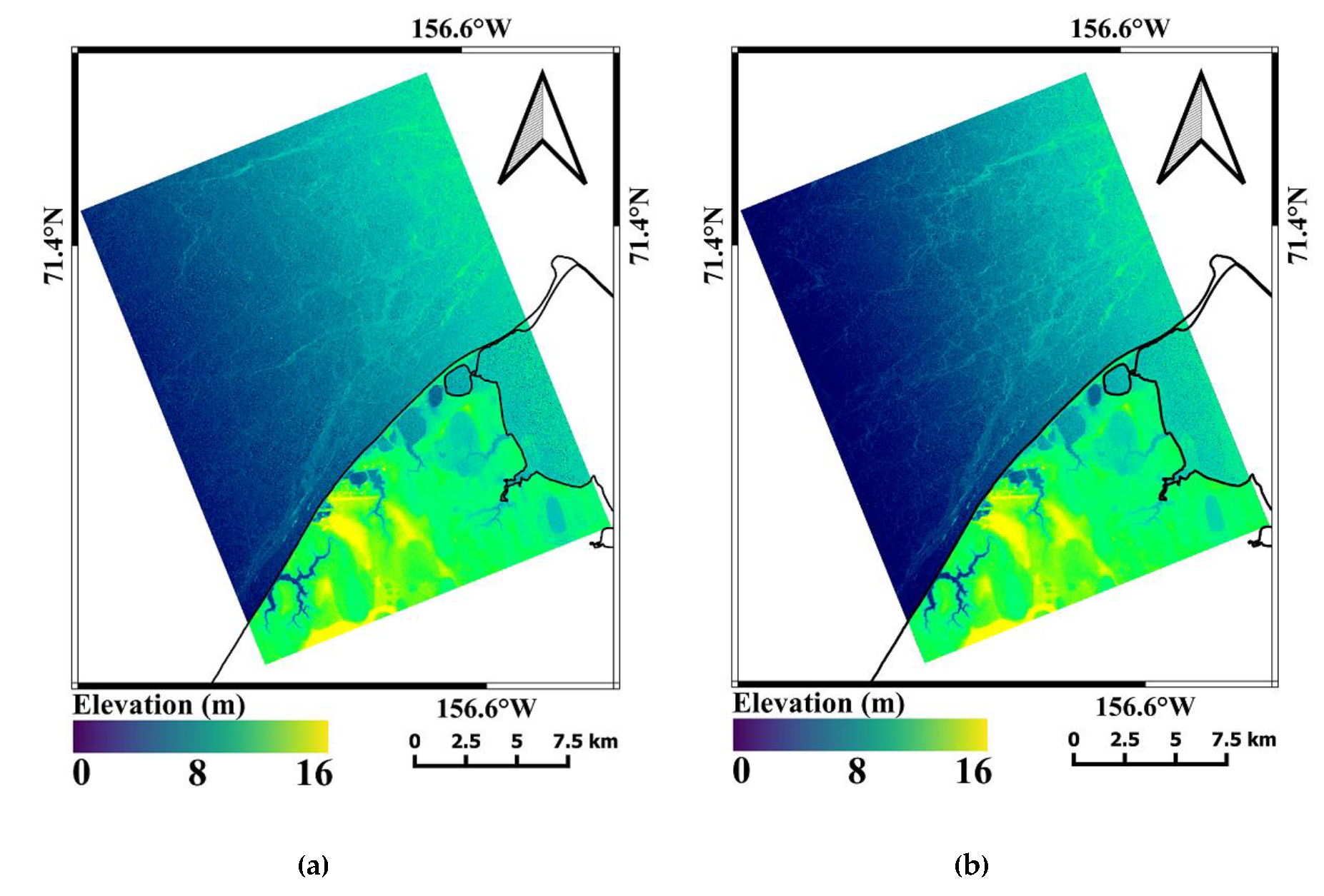
3.2. Generation of a Height Difference Map (HDM)

In this study, we used two TanDEM-X scenes from 13 and 24 Jan 2012. These particular scenes were selected based on:

• Time period of active landfast ice deformation and ridging.
• Bistatic acquisitions resulting in a short (~10 ms) temporal baseline reducing $∆{\varnothing }_{\mathit{mov}}$ to a minimum.
• Temperatures consistently below 0 °C to avoid surface change and coherence loss due to melt.
• A small HOA resulting in significant height sensitivity and a topographic signal exceeding that of the noise floor.

The generation of the HDM involved deriving a DEM for both days through the following processing steps: interferogram formation, multilooking (3 × 3) to reduce phase noise, phase unwrapping using Statistical-cost Network-flow Algorithm for PHase Unwrapping (SNAPHU), DEM generation based on the HOA, and filtering (boxcar 5 × 5) of the elevation maps (Figure 3) to enhance the appearance of ridges.

We coregistered the DEMs before calibrating from relative to absolute height based on a known reference point (the Utqiaġvik airport) and projected into Universal Transverse Mercator (UTM) zone 4N (Figure 3). The DEMs exhibit significant elevation gradients in the range direction, which are caused by phase ramps known to occur in TanDEM-X data [43,44,45,46,47] (Figure 4a). In our case, this effect is most likely due to inaccuracies in the across-track baseline ($∆{\varnothing }_{\mathit{error}}$ in Equation (1)), but a phase ramp can also occur due to a non-zero $∆{\varnothing }_{\mathit{prop}}$ resulting in a different path length across the scene. After the difference between the two DEMs was calculated (Figure 4a), the remaining elevation gradient was removed from the HDM by averaging all pixels covering land for each pixel row in the along-track direction. In the case where there is no phase ramp, this mean is expected to be close to zero. We removed the mean for each full row and filtered the final product (boxcar 3 × 3 pixels), resulting in an HDM without a noticeable height ramp and reduced noise (Figure 4b). The resolution of the HDM is 7 m.

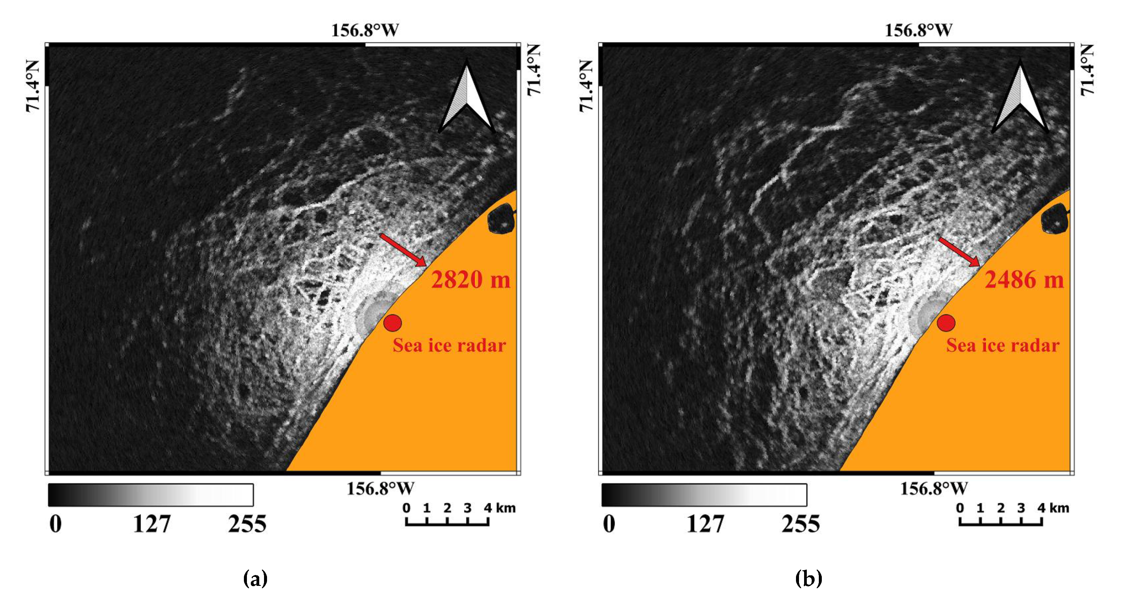
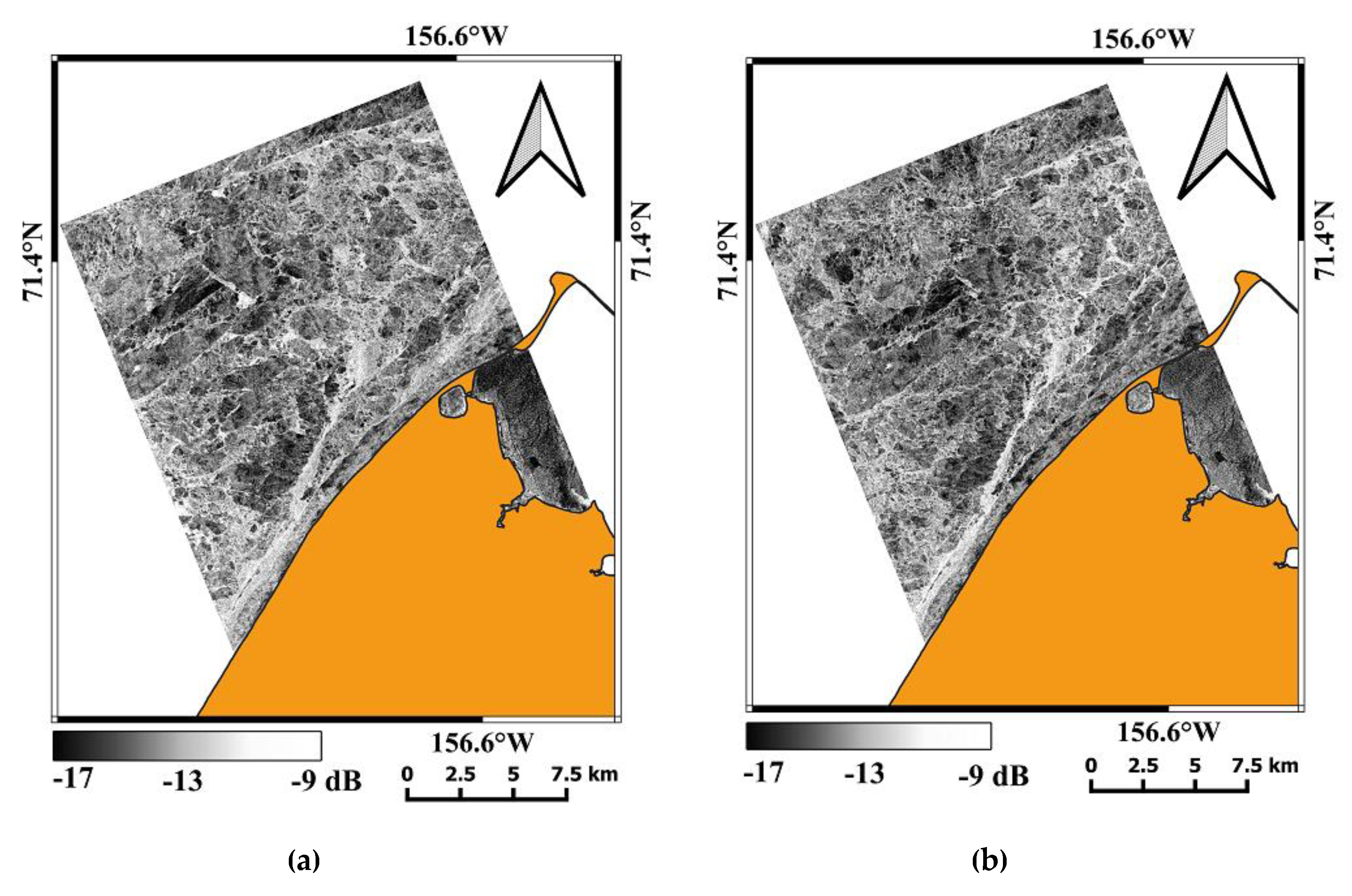
3.3. Backscatter Intensity

In addition to the interferometric phase, we also considered the backscatter information. This signal depends on characteristics of the ice surface, including the dielectric properties as well as the cm- and m-scale surface roughness [48]. Ridges are therefore visible in backscatter imagery and are used here for comparison.

We base our analysis on the reflectivity per unit area in slant range, i.e., the radar brightness ${\beta }^{°}$ calculated from the image pixel values or digital numbers (DN) applying a calibration factor $k_s$:

$${\beta }^{°}=k_s · \left|D{N}^2\right|$$

(5)

and converted ${\beta }^{°}$ to dB scale:

$${\beta }_{dB}^{°}=10 · {\mathit{log}}_{10}\left({\beta }^{°}\right)$$

(6)

before applying a Lee Speckle noise filter with a filter kernel of 5 × 5 pixels (Figure 5).

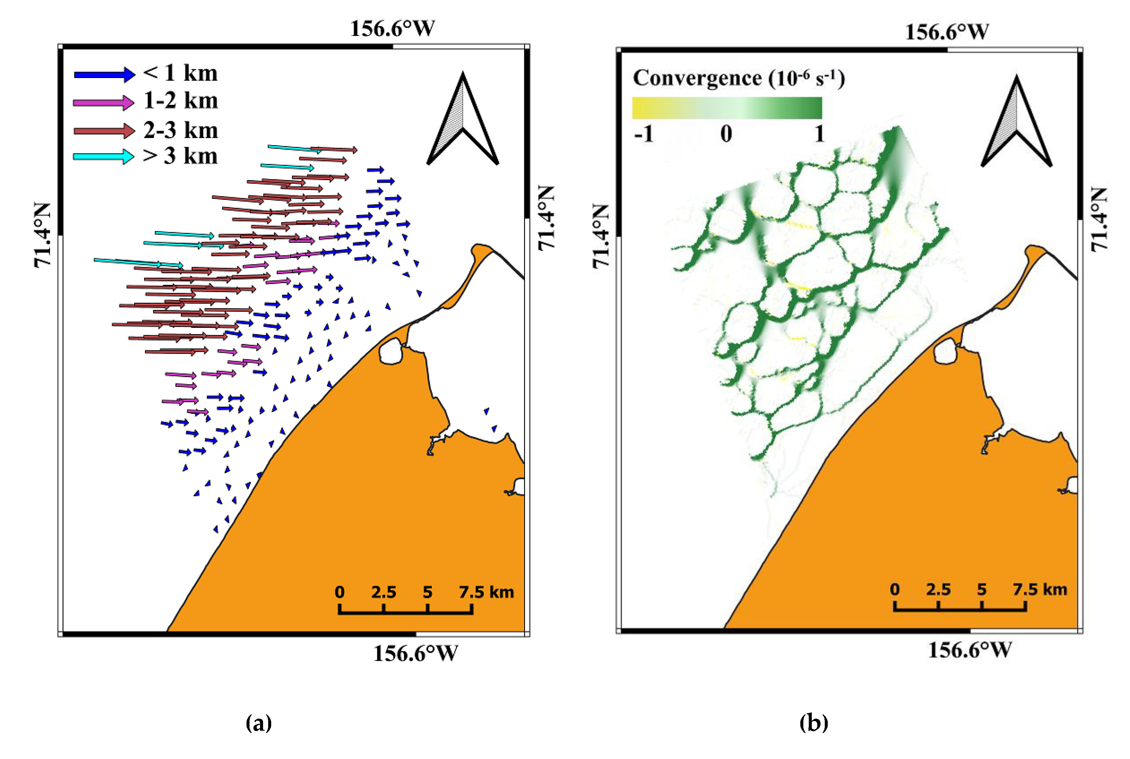
3.4. Sea Ice Drift Estimation

When drifting pack ice comes in contact with landfast ice, it can result in cm-scale ice fracturing or large m-scale deformation in terms of rafting and riding events. Sea ice drift is therefore of relevance and can be evaluated using SAR [49] through ice drift algorithms [35,50,51]. Here, we applied an algorithm based on SAR backscatter and specifically areal matching by phase correlation and feature tracking [35]. This method enables robust identification and tracking of translational as well as rotational motion of the image structures. Drift vectors were calculated with a grid spacing of 10 pixels, i.e., 80 m. The sea ice drift between 13 and 24 Jan is displayed in Figure 6a. Based on this drift field, we derived the convergence [52] as a result of the onshore compression (Figure 6b), which indicates likely areas of ridge formation.

4. Results

The SAR-derived drift indicates that the predominant ice motion is roughly towards the east (Figure 6a). The onshore drift is thus in agreement with the wind direction and is also confirmed by the ground-based radar (Figure 2). The HDM indicates locations of either ridge displacement or formation events between 13 and 24 Jan 2012 (Figure 4b). Ridge displacement can be identified through a positive elevation change near a similar pattern of negative elevation change where the ridge used to be. We focused on four areas of ridge displacement (numbered D1–4 in Figure 4b). In these locations, blue features indicate locations of ridges on 13 Jan and red features ridge locations on 24 Jan. To compare the displacement observed in the HDM with the output from the ice drift algorithm, the locations of the ice drift vectors were matched with the identified displacements in the HDM. Drift vectors with starting points on the blue features were selected and are displayed as green arrows in Figure 7, Figure 8, Figure 9 and Figure 10. The averages of the extracted ice drift vectors were calculated for each ridge displacement and are represented by yellow arrows. For each displacement, we also identified five control points (i.e., distinct points along the ridge that can be recognized prior to and after displacement). In Figure 7, Figure 8, Figure 9 and Figure 10, the control points are denoted as ‘a’ prior to displacement and ‘b’ after displacement. Distances from ‘a’ to ‘b’ were measured and the averages for each displacement were calculated (not shown in figures). Finally, these control point averages were compared with the drift vector averages (yellow arrows). The formation of ridges can be identified by a positive elevation change but lack a similar stark nearby negative response. Here, we focused on two areas of ridge formation (numbered F1–2 in Figure 4b).

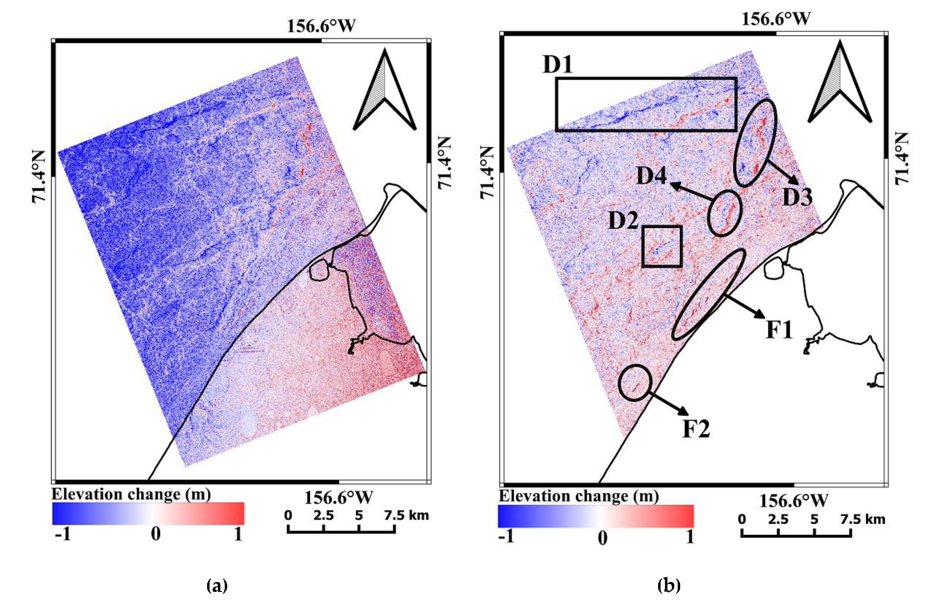
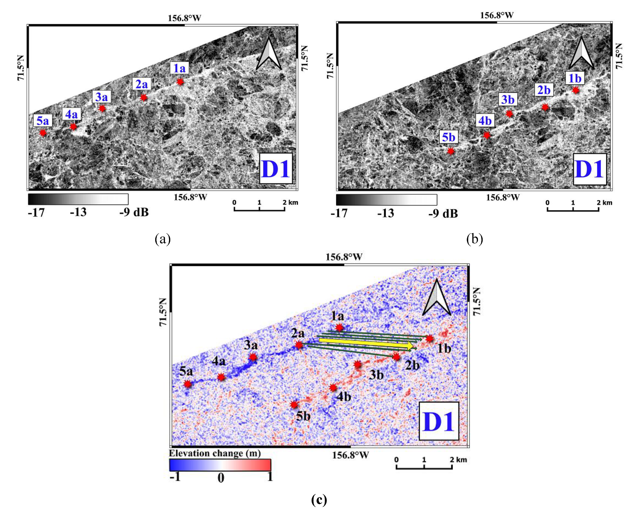
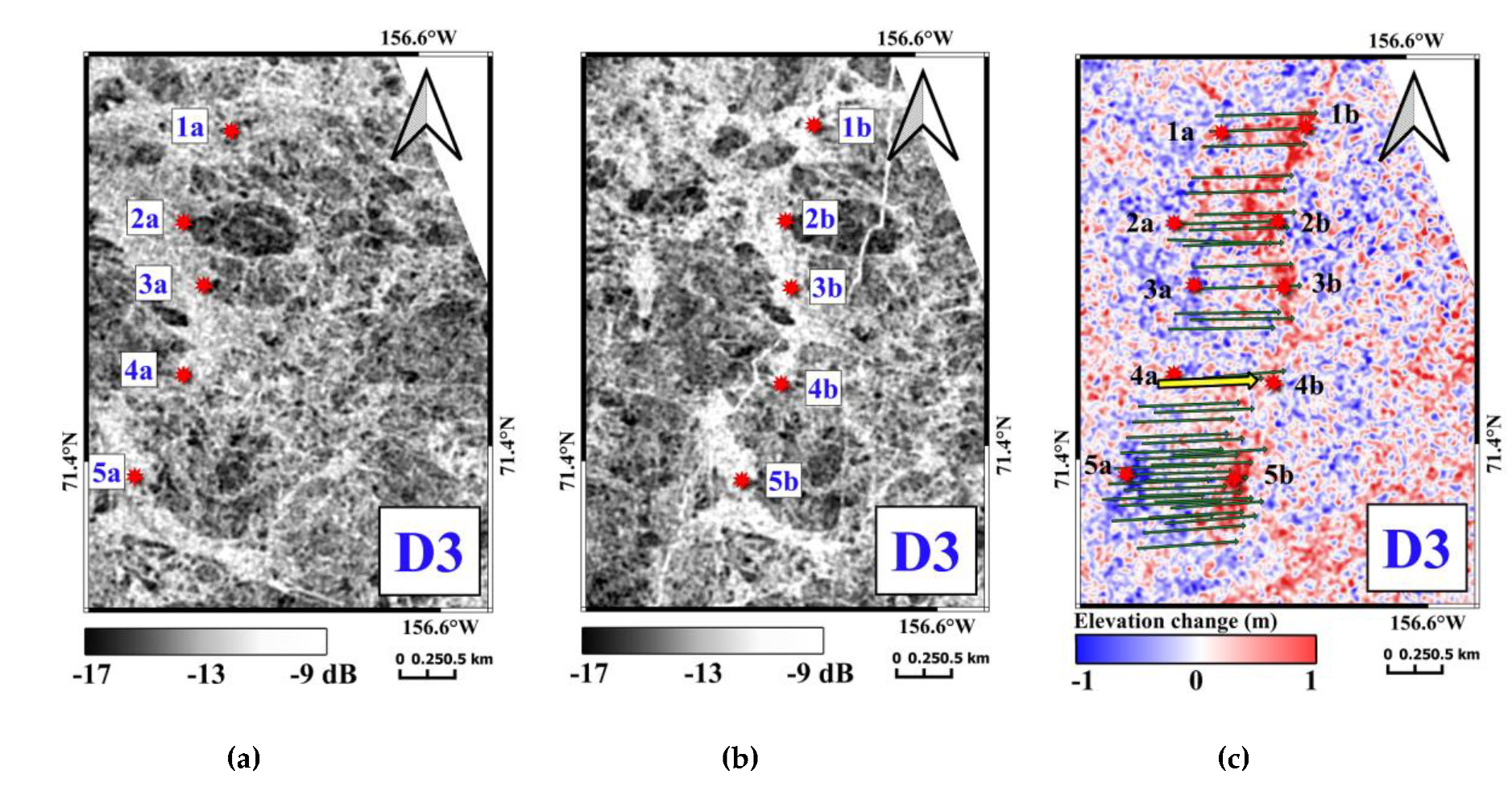
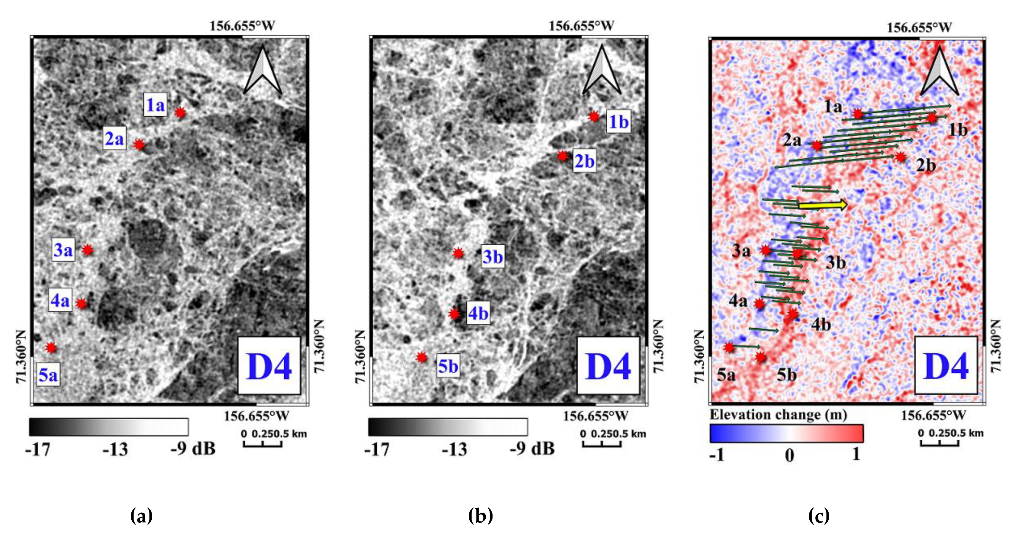
4.1. Detection of Ridge Displacement

D1 represents a clear example of ridge displacement (Figure 4b). Control points 1–5 represent features of the ridge that can be recognized in both backscattering images (Figure 7a,b) and also the HDM (Figure 7c). Ridge features were barely detectable in the coastal radar imagery due to low backscatter near the edge of the radar range (not shown). The points a and b that are labeled on control points 1–5 show the location of ridges on 13 and 24 Jan, respectively.

Based on the control points in the SAR backscatter images and the HDM, the average displacement between points 1a–5a and 1b–5b is 3.7 km towards the coast (Figure 7a,b). We tried to compare the average displacement between control points with vectors of the drift algorithm for the whole D1 displacement, but we were only able to extract seven drift vectors covering the control points 1a–2a and 1b–2b. The reason for this is that D1 is located at the image border where the performance of the ice drift algorithm is limited. The seven available drift vectors suggest an average displacement of 3.4 km. This displacement is the same as the displacement measured based on the control points 1a–2a and 1b–2b, i.e., 3.4 km.

D2 is located near the center of our study area (Figure 4b). We identified five control points (Figure 8a,b in backscatter intensity images and Figure 8c,d in coastal radar images) indicating an average displacement of 1.0 km using control points. In this case, the ridge displacement is not as apparent in the backscatter as in D1, but the displacement is clearly visible in the HDM in the location of the control points (Figure 8e) and also coastal radar images (Figure 8c,d). We were able to identify a total of 13 vectors with the drift algorithm indicating an average displacement of 1.0 km (yellow vector in Figure 8e), nearly identical to what we derived based on the backscatter and coastal radar control points (control point averages were also nearly 1 km).

D3 and D4 represent two locations along the same ridge. In D3, we identify five control points on the backscatter imagery (Figure 9a,b). The HDM clearly indicates a shift corresponding to the shift indicated by the control points at 0.9 km (Figure 9c). The drift algorithm identified a total of 41 vectors along the ridge with a resulting mean displacement of 0.9 km compared to that indicated in the control points and the HDM (Figure 9c).

For D4, as for D3, five control points were identified on the backscatter imagery (Figure 10a,b). The HDM clearly indicates a shift corresponding to the shift indicated by the control points at 0.7 km. The drift algorithm identified a total of 46 vectors along the ridge with a resulting mean displacement of 0.6 km, similar to that indicated in the control points and the HDM (Figure 10c). We were not able to detect the ridge in D3 and D4 in the coastal radar imagery likely due to radar signal disturbance from surrounding rough ice in the near range and a low signal in the far range (not shown).

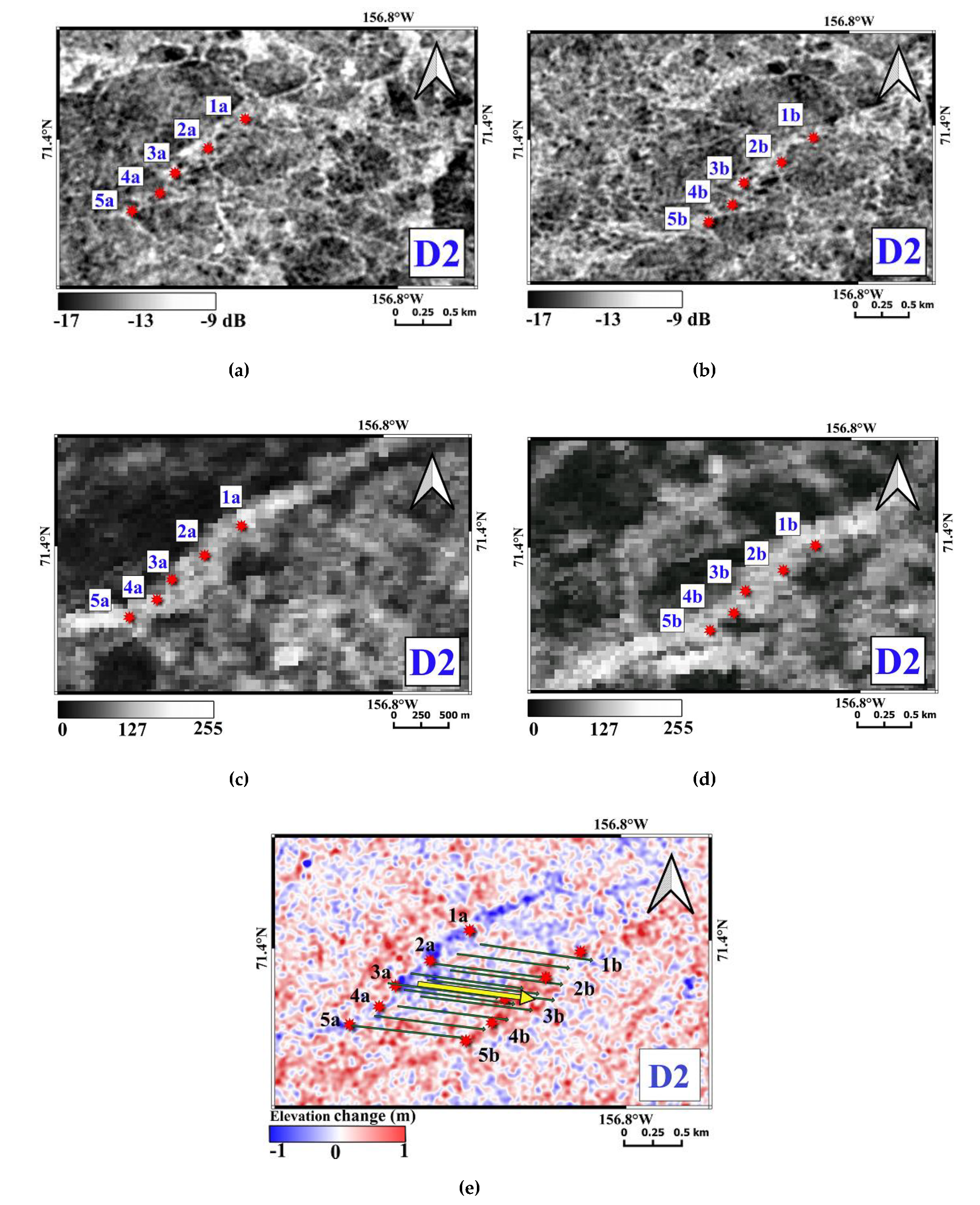
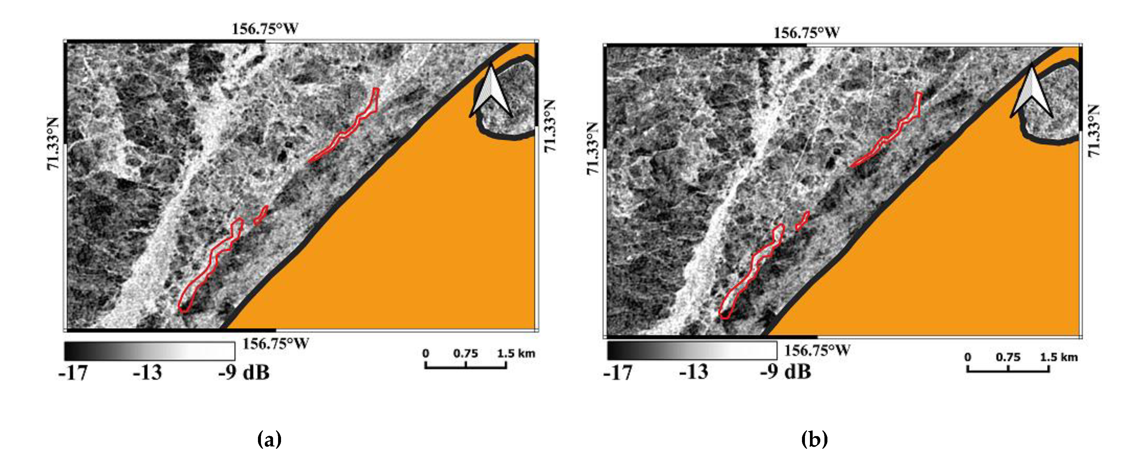
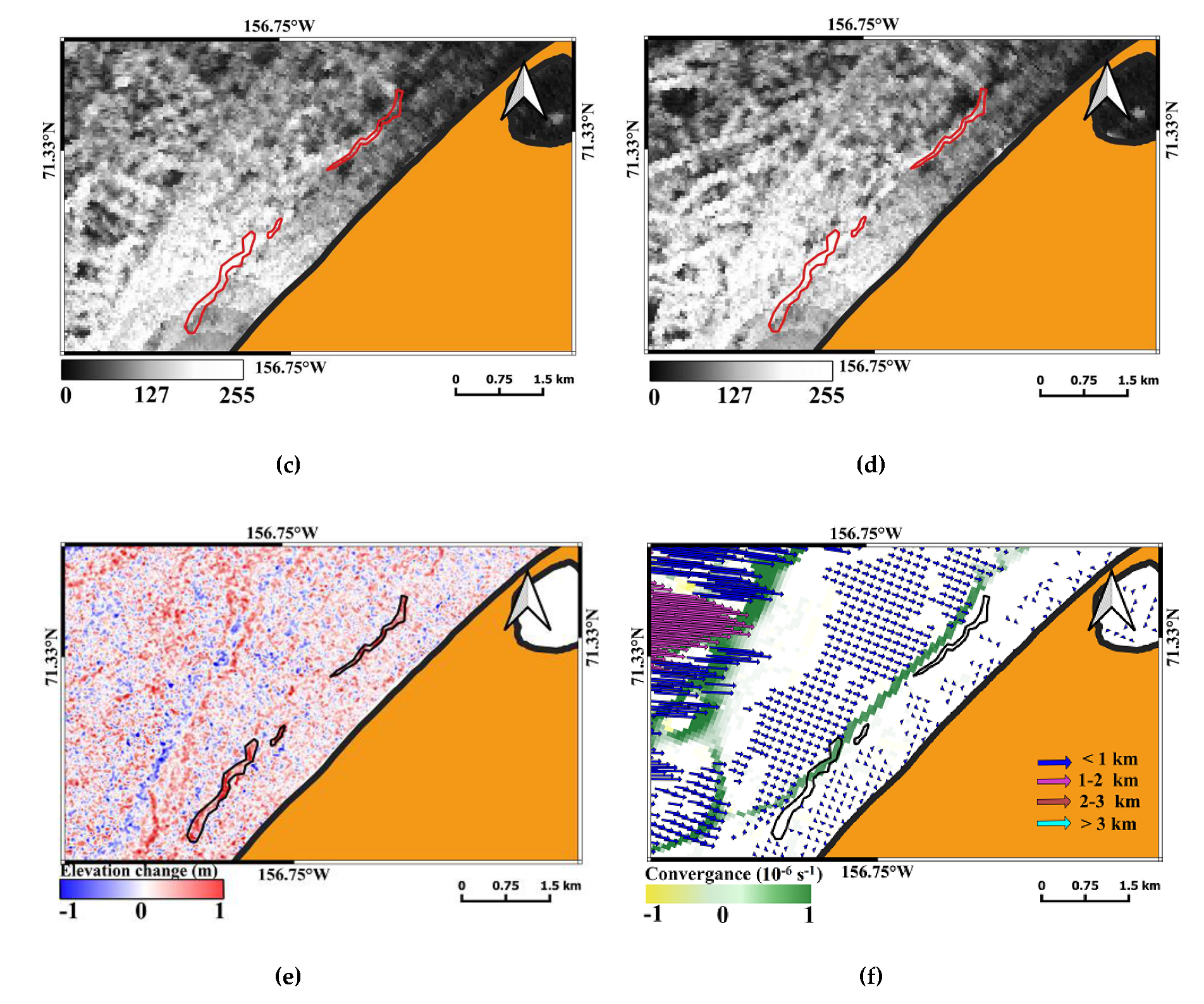
4.2. Detection of Ridge Formation

We identified and analyzed two cases of ridge formation between 13 and 24 Jan 2012 (F1 and F2). Similar to scenario D1–4, we compared SAR backscatter and coastal radar data with the HDM. In addition, we also compared these scenarios with convergence/divergence zones as identified by the drift algorithm (Figure 6b).

F1 represents a combination of several ridges forming close to the coast. The backscatter image on 13 Jan indicates that a ridge was already present (red outline in Figure 11a). Therefore, it is difficult to detect any ridge development in the area by strictly evaluating the backscatter imagery, which only slightly increased in backscatter coefficient during the time between acquisitions (−12.4 to −12.2 dB). However, by evaluating the elevation difference (black outline in Figure 11e), the ridge has increased by up to one meter during the time between acquisitions. We further evaluated the convergence results from the drift algorithm (Figure 11f). Here, we identified substantial convergence of roughly 10⁻⁶ s⁻¹ within ~200 m of the location of the stark elevation changes (black outline in Figure 11e). This corresponds to a convergence rate of ~1 during the 11-day timespan, indicating that for every meter of ice, it is compressed by roughly 1 m. Ice thickness was also found to be close to 1 m (Section 2.1). Hence, the increase in ridge height by up to 1 m is plausible if we assume that the resulting rubble/small ridge ends up resting on surrounding ice leading to minimal draft. The area of the convergence and the elevated ridge do not overlap perfectly, which is likely a result of a combination of ridge buildup and displacement in one event. This leads to the final ridge ending up closer to shore than the location at which it first started forming.

F2 is located in the southwest part of the study region (Figure 4b). Similar to F1, it is difficult to determine whether there has been active ridge development strictly based on subtle changes in average backscatter values from −12.4 to −11.8 dB (within the red outline in Figure 12a,b). However, it is clear from the elevation change that a ridge has developed from either a pre-existing ridge or a rubble field (black outline in Figure 12e). Once again, we compared the ridge development with the drift product. Here the ridge development can also be explained by the observed onshore displacement and convergence ~300 m seaward of the identified ridge development likely a result of combined ridge buildup and displacement in one process (Figure 12f).

Ridges can form in rough ice conditions and hence ridging events can be difficult to detect from backscatter alone. This is due to the pre-existing high backscatter from ice rubble. This is apparent in our analysis of both SAR (Figure 11a,b for F1 and Figure 12a,b for F2) and coastal radar backscatter (Figure 11c,d for F1 and Figure 12c,d for F2) where it is difficult to determine exactly where the ridges are forming. The interferometric height change helps determine in what areas compression leads to ridge formation and what areas remain or develop into rubble fields. With this said, both areas of elevated interferometric height (F1 and F2) also exhibit elevated backscatter values during the timespan analyzed, lending support to the interferometric results of ridge formation in these locations.

5. Discussion

This study evaluated the possibility of identifying the development and displacement of ice ridges in landfast sea ice using single-pass InSAR measurements by TanDEM-X. We utilized ground-based radar data that helped identify riding events and initially evaluate our approach. Additional ground truth data or data obtained by other sensors of sea ice surface topography were not available for the studied area and time period. We verified results based on backscatter intensity values, coastal radar data, ice displacement vectors, and convergence fields using a SAR-based sea ice drift algorithm. A qualitative comparison exhibits the agreement between the different datasets evaluated, which demonstrates the application of deriving sea ice surface elevation changes using InSAR.

The majority of the published InSAR studies focus on landfast ice, which under favorable conditions allows the use of repeat pass InSAR without complete decorrelation e.g., [18,25,53,54,55]. Here we applied TanDEM-X, from which close orbit formation enables acquisition of highly accurate cross-track and/or along-track interferograms without inherent accuracy limitations imposed by repeat-pass interferometry due to temporal decorrelation effects and atmospheric disturbances [31,33]. Therefore, although the results presented here reveal the feasibility and potential of the proposed technique for landfast ice, the approach may also be applicable for drifting ice with a few limitations. First, to apply InSAR for drifting ice, the temporal separation between the SAR acquisitions must be short enough to avoid coherence loss, which requires use of single-pass InSAR for generation of the height maps. Second, the method presented here would require co-registration of individual ridges as they would have moved during the time between acquisitions. Third, the impacts of motion on the interferometric phase needs to be removed from the analysis to avoid significant reductions in accuracy.

The use of this approach on non-stationary ice may be particularly relevant in locations where sea ice motion is restricted (e.g., in fjords or bays), hence ridges can be identified in two consecutive TanDEM-X acquisitions spanning an 11-day time period. However, the approach would still require careful selection of image pairs with an appropriate spatial baseline, which places further limitations on already limited data availability. The use of this technique for non-restricted free-drifting ice would be challenging, but is theoretically possible for ice floes that can be identified in two different TanDEM-X acquisitions and co-registered, so that the ridge formation analysis can be performed. If more single-pass InSAR systems will be available in the future, it should also be possible to analyze the difference between height maps from different satellite systems. This would make it possible to select time intervals that are shorter than the 11 days that are given by the TanDEM-X orbit.

The application of InSAR-derived absolute ridge height has been demonstrated in past work [20,31], as well as the dm-scale accuracy of TanDEM-X-derived ice topography [34]. Depending on coherence and baselines, InSAR is therefore most relevant for evaluation of larger ridges several meters in height as opposed to rafting and other cm-scale changes in ice roughness. Here, we took this work a step further and derived relative HDMs between two InSAR generated DEMs each with an accuracy of one meter. This approach will possibly be suitable for evaluating volumetric changes in ridges by integrating over the area of the ridge itself. This could provide value for understanding ridging dynamics and the relationship between ice thickness, convergence, and ridge development and resulting size, density, and morphology. To explore this further would require validation with in situ measurements.

In general, radar signatures of deformation features, including ice ridges at C- and L-band frequencies, are characterized by large backscatter intensities and significant variation in SNR across short distances [31]. The advantage of the strong contrast is that a larger variation of different deformation features can be detected, particularly at L-band frequencies [56]. On the other hand, the significant variation of SNR leads to a higher relative error in sail height retrieval. At higher frequencies, such as X-band, this effect is less pronounced because radar backscattering from level ice surfaces with small mm- to cm-scale ice roughness is stronger, resulting in smaller intensity contrasts between deformed and smooth ice [31]. Consequently, the smaller wavelength in a combination with higher return signal from smooth ice is advantageous in comparison with L- and C-bands due to higher vertical resolution and lower relative height error.

Although the number of satellites that can deliver repeat-pass InSAR data is increasing, the TanDEM-X constellation is currently the only available system for spaceborne single-pass InSAR assessments of sea ice topography. This will likely change in the future when the number of small and relatively affordable satellites increases. There are initiatives to create single pass InSAR systems by letting a small passive SAR satellite fly in close formation with a larger active SAR satellite like the Sentinel-1. There is also a proposal for a TanDEM-L mission, which is similar to TanDEM-X, but featuring an L-band sensor (λ = 25 cm). With increasing potential for a commercial market for single-pass InSAR products, it is also plausible that commercial providers of small low-cost SAR satellites will offer an alternative suitable for single-pass InSAR.

6. Conclusions

In this paper, we analyzed for the first time the application of InSAR for assessing ridge formation and displacement in landfast sea ice using interferometric change detection. In this effort, we analyzed the phase signatures of two single-pass bistatic X-band SAR image pairs acquired on the 13th and 24th of January 2012 near Utqiaġvik, Alaska. The resulting elevation change product compared favorably with backscatter–intensity features, coastal radar imageries, and ice drift information generated by a SAR-based sea ice tracking algorithm. We identified a total of six cases of ridge displacement and formation under onshore compression. Ridge displacement ranged between roughly 0.6 and 3.7 km and ridge formation resulted in upwards of 1 m vertical buildup. These areas correspond with areas identified as convergence zones in derived drift products, as well as ground-based radar imagery, lending confidence to this approach in providing valuable information related to ice ridging events.

Future work is needed to evaluate the accuracy of this approach and will need to include the collection of in situ measurements. The sensitivity of the approach to orbit parameters (e.g., local incident angle, baselines) and ice regimes (e.g. salinity, morphology, season) should also be taken into account to determine robustness of this approach and expected accuracy values. Consequently, such analysis will help determine the application of this approach for assessing volumetric changes as a result of ridging. Such information is needed to estimate ridge porosity and structural integrity relevant in the context of internal ridge strength, landfast ice stability, and potential impact on vessels and structures.

The limitations and open questions related to this approach, in particularly related to data availability, currently hamper the use for ice management and operational applications. However, the method can currently be applied to investigate ice deformation and dynamics. This is of key relevance for understanding the engineering properties of sea ice across large spatial scales, which are difficult to determine based on in situ or laboratory experiments. This method can also be used to investigate the ice/atmosphere/ocean forcing conditions under which different types of ridges form and where/when convergence leads to ridge displacement, formation of new ridges, or development of existing features. Such information is currently difficult to obtain or evaluate at the needed spatial scale. Here, InSAR can potentially provide new and valuable insight which can be used to further understand ice properties and stability, and potentially help guide the development of landfast sea ice models.

References

1. Eicken, H.; Lovecraft, A.L.; Druckenmiller, M.L. Sea-ice system services: A framework to help identify and meet information needs relevant for Arctic observing networks. Arctic 2009, 62, 119–136. [Google Scholar] [CrossRef] [Green Version]
2. Dammann, D.O.; Eicken, H.; Mahoney, A.; Meyer, F.; Betcher, S. Assessing sea ice trafficability in a changing Arctic. Arctic 2018, 71, 59–75. [Google Scholar] [CrossRef]
3. Reimnitz, E.; Dethleff, D.; Nürnberg, D. Contrasts in Arctic shelf sea-ice regimes and some implications: Beaufort Sea vs Laptev Sea. Mar. Geol. 1994, 119, 215–225. [Google Scholar] [CrossRef]
4. Reimnitz, E.; Maurer, D. Effects of storm surges on the Beaufort Sea Coast, Northern Alaska. Arctic 1979, 32, 329–344. [Google Scholar] [CrossRef] [Green Version]
5. Wilson, K.; Falkingham, J.; Melling, H.; De Abreu, R. Shipping in the Canadian Arctic-other possible climate scenarios. In Proceedings of the IEEE International Geoscience and Remote Sensing Symposium, Anchorage, AK, USA, 20–24 September 2004. [Google Scholar]
6. Divine, D.; Korsnes, R.; Makshtas, A. Temporal and spatial variation of shorefast ice in the Kara Sea. Cont. Shelf. Res. 2004, 24, 1717–1736. [Google Scholar] [CrossRef]
7. Eicken, H.; Dmitrenko, I.; Tyshko, K.; Darovskikh, A.; Dierking, W.; Blahak, U.; Groves, J.; Kassens, H. Zonation of the Laptev Sea landfast ice cover and its importance in a frozen estuary. Global Planet. Chang. 2004, 48, 55–83. [Google Scholar] [CrossRef]
8. Jones, J.; Eicken, H.; Mahoney, A.; MV, R.; Kambhamettu, C.; Fukamachi, Y.; Ohshima, K.; George, J.C. Landfast sea ice breakouts: Stabilizing ice features, oceanic and atmospheric forcing at Barrow, Alaska. Cont. Shelf. Res. 2016, 126, 50–63. [Google Scholar] [CrossRef] [Green Version]
9. Zubov, N.N. Arctic Sea Ice; English Translation 1963 from Russian Language by U.S.; Naval Oceanographic Office and American Meteorological Society: San Diego, CA, USA, 1945; p. 491. [Google Scholar]
10. Mahoney, A.; Eicken, H.; Gaylord, A.G.; Gens, R. Landfast sea ice extent in the Chukchi and Beaufort Seas: The annual cycle and decadal variability. Cold Reg. Sci. Technol. 2014, 103, 41–56. [Google Scholar] [CrossRef]
11. Mahoney, A.; Eicken, H.; Graves-Gaylord, A.; Shapiro, L. Alaska landfast sea ice: Links with bathymetry and atmospheric circulation. J. Geophys. Res. 2007, 112, 1–18. [Google Scholar] [CrossRef] [Green Version]
12. Gearheard, S.; Matumeak, W.; Angutikjuaq, I.; Maslanik, J.; Huntington, H.; Leavitt, J.; Kagak, D.M.; Tigullaraq, G.; Barry, R. “It’s not that simple”: A collaborative comparison of sea ice environments, their uses, observed changes, and adaptations in Barrow, Alaska, USA, and Clyde River, Nunavut, Canada. AMBIO A J. Hum. Environ. 2006, 35, 203–211. [Google Scholar] [CrossRef]
13. George, J.C.; Huntington, H.; Brewster, K.; Eicken, H.; Norton, D.; Glenn, R. Observation on shorefast ice dynamics in northern Alaska and the responses of the Iñupiat hunting community. Arctic 2004, 57, 363–374. [Google Scholar] [CrossRef]
14. George, J.C.; Zeh, J.; Suydam, R.; Clark, C. Abundance and population trend (1978–2001) of western arctic bowhead whales surveyed near Barrow, Alaska. Mar. Mamm. Sci. 2006, 20, 755–773. [Google Scholar] [CrossRef]
15. Sonnenfeld, J. Changes in Subsistence Among the Barrow Eskimo. Ann. Assoc. Am. Geogr. 1960, 50, 172–186. [Google Scholar] [CrossRef]
16. Mahoney, A.; Eicken, H.; Shapiro, L. How fast is landfast sea ice? A study of the attachment and detachment of nearshore ice at Barrow, Alaska. Cold Reg. Sci. Technol. 2007, 47, 233–255. [Google Scholar] [CrossRef]
17. Druckenmiller, M.L. Alaska Shorefast Ice: Interfacing Geophysics with Local Sea Ice Knowledge and Use. Ph.D. Thesis, University of Alaska Fairbanks, Fairbanks, AK, USA, 2011. [Google Scholar]
18. Dammann, D.O.; Eriksson, L.E.B.; Mahoney, A.R.; Eicken, H.; Meyer, F.J. Mapping pan-Arctic landfast sea ice stability using Sentinel-1 interferometry. Cryosphere 2019, 13, 557–577. [Google Scholar] [CrossRef] [Green Version]
19. Barker, A.; Timco, G.; Wright, B. Traversing grounded rubble fields by foot—Implications for evacuation. Cold Reg. Sci. Technol. 2006, 46, 79–99. [Google Scholar] [CrossRef]
20. Dammann, D.O.; Eicken, H.; Mahoney, A.R.; Saiet, E.; Meyer, F.J.; George, J.C. Traversing Sea Ice—Linking Surface Roughness and Ice Trafficability Through SAR Polarimetry and Interferometry. IEEE J. Sel. Top. Appl. 2018, 11, 416–433. [Google Scholar] [CrossRef]
21. Druckenmiller, M.L.; Eicken, H.; George, J.C.; Brower, L. Trails to the whale: Reflections of change and choice on an Iñupiat icescape at Barrow, Alaska. Polar Geogr. 2013, 36, 5–29. [Google Scholar] [CrossRef]
22. Dierking, W. Laser profiling of the ice surface topography during the Winter Weddell Gyre Study. J. Geophys. Res. Oceans 1992, 100, 4807–4820. [Google Scholar] [CrossRef]
23. Farrell, S.L.; Markus, T.; Kwok, R.; Connor, L. Laser altimetry sampling strategies over sea ice. Ann. Glaciol. 2011, 52, 69–76. [Google Scholar] [CrossRef] [Green Version]
24. Kwok, R.; Zwally, H.J.; Yi, D. ICESat observations of Arctic sea ice: A first look. Geophysical. Res. Lett. 2004, 31, 1–5. [Google Scholar] [CrossRef] [Green Version]
25. Dammert, P.B.G.; Lepparanta, M.; Askne, J. SAR interferometry over Baltic Sea ice. Int. J. Remote Sens. 1998, 19, 3019–3037. [Google Scholar] [CrossRef]
26. Meyer, F.J.; Mahoney, A.R.; Eicken, H.; Denny, C.L.; Druckenmiller, H.C.; Hendricks, S. Mapping arctic landfast ice extent using L-band synthetic aperture radar interferometry. Remote Sens. Environ. 2011, 115, 3029–3043. [Google Scholar] [CrossRef]
27. Dammann, D.O.; Eicken, H.; Meyer, F.; Mahoney, A. Assessing small-scale deformation and stability of landfast sea ice on seasonal timescales through L-band SAR interferometry and inverse modeling. Remote Sens. Environ. 2016, 187, 492–504. [Google Scholar] [CrossRef] [Green Version]
28. Dammann, D.O.; Eicken, H.; Mahoney, A.; Meyer, F.; Freymueller, J.; Kaufman, A.M. Assessing landfast sea ice stability and internal ice stress around ice roads using L-band SAR interferometry and inverse modeling. Cold. Reg. Sci. Technol. 2018, 149, 51–64. [Google Scholar] [CrossRef]
29. Dammann, D.O.; Eicken, H.; Mahoney, A.; Meyer, F.; Eriksson, L.; Saiet, E.; Freymueller, J.; Jones, J. New Possibilities Using TSX and TDX in Support of Sea Ice Use. In Proceedings of the European Conference on Synthetic Aperture Radar, Aachen, Germany, 4–7 June 2018. [Google Scholar]
30. Mahoney, A.R.; Dammann, D.O.; Johnson, M.A.; Eicken, H.; Meyer, F.J. Measurement and imaging of infragravity waves in sea ice using InSAR. Geophys. Res. Lett. 2016, 43, 6383–6392. [Google Scholar] [CrossRef] [Green Version]
31. Dierking, W.; Lang, O.; Busche, T. Sea ice local surface topography from single-pass satellite InSAR measurements: A feasibility study. Cryosphere 2017, 11, 1967–1985. [Google Scholar] [CrossRef] [Green Version]
32. Yitayew, T.; Dierking, V.; Divine, D.V.; Eltoft, T.; Ferro-Famil, L.; Rösel, A.; Negrel, J. Validation of Sea-Ice Topographic Heights Derived From TanDEM-X Interferometric SAR Data With Results From Laser Profiler and Photogrammetry. IEEE Trans. Geosci. Remote Sens. 2018, 56, 6504–6520. [Google Scholar] [CrossRef]
33. Dammann, D.O.; Eriksson, L.E.; Jones, J.M.; Mahoney, A.R.; Romeiser, R.; Meyer, F.J.; Eicken, H.; Fukamachi, Y. Instantaneous sea ice drift speed from TanDEM-X interferometry. Cryosphere 2019, 13, 1395–1408. [Google Scholar] [CrossRef]
34. Dammann, D.O.; Eriksson, L.E.B.; Nghiem, S.V.; Pettit, E.C.; Kurtz, N.T.; Sonntag, J.G.; Busche, T.E.; Meyer, F.J.; Mahoney, A.R. Iceberg topography and volume classification using TanDEM-X interferometry. Cryosphere 2019, 13, 1861–1875. [Google Scholar] [CrossRef] [Green Version]
35. Berg, A.; Eriksson, L.E. Investigation of a hybrid algorithm for sea ice drift measurements using synthetic aperture radar images. IEEE Trans. Geosci. Remote Sens. 2013, 52, 5023–5033. [Google Scholar] [CrossRef] [Green Version]
36. Mahoney, A.R.; Eicken, H.; Fukamachi, Y.; Ohshima, K.I.; Simizu, D.; Kambhamettu, C.; Rohith, M.; Hendricks, S.; Jones, J. Taking a look at both sides of the ice: Comparison of ice thickness and drift speed as observed from moored, airborne and shore-based instruments near Barrow, Alaska. Ann. Glaciol. 2015, 56, 363–372. [Google Scholar] [CrossRef] [Green Version]
37. Rohith, M.; Jones, J.; Eicken, H.; Kambhamettu, C. Extracting Quantitative Information on Coastal Ice Dynamics and Ice Hazard Events from Marine Radar Digital Imagery. IEEE Trans. Geosci. Remote Sens. 2013, 51, 2556–2570. [Google Scholar]
38. Jones, J.M. Landfast Sea Ice Formation and Deformation Near Barrow. Master’s Thesis, University of Alaska Fairbanks, Fairbanks, AK, USA, 2013. [Google Scholar]
39. Druckenmiller, M.L.; Eicken, H.; Johnson, M.A.; Pringle, D.J.; Williams, C.C. Toward an integrated coastal sea-ice observatory: System components and a case study at Barrow, Alaska. Cold Reg. Sci. Technol. 2009, 56, 61–72. [Google Scholar] [CrossRef]
40. Maurer, E.; Kahle, R.; Mrowka, F.; Ohndorf, A.; Zimmermann, S. Operational aspects of the TanDEM-X Science Phase. In Proceedings of the 14th International Conference on Space Operations, Daejeon, Korea, 16–20 May 2016. [Google Scholar] [CrossRef] [Green Version]
41. Krieger, G.; Moreira, A.; Fielder, H.; Hajnsek, I.; Werner, M.; Younis, M.; Zink, M. TanDEM-X: A satellite formation for high-resolution SAR interferometry. IEEE Trans. Geosci. Remote. Sens. 2007, 45, 3317–3341. [Google Scholar] [CrossRef] [Green Version]
42. Rosen, P.A.; Hensley, S.; Joughin, I.R.; Li, F.K.; Madsen, S.N.; Rodriguez, E.; Goldstein, R.M. Synthetic aperture radar interferometry. Proc. IEEE. 2000, 88, 333–382. [Google Scholar] [CrossRef]
43. Elyouncha, A.; Eriksson, L.E.B.; Romeiser, R.; Ulander, L.M.H. Measurements of Sea Surface Currents in the Baltic Sea Region Using Spaceborne Along-Track InSAR. IEEE Trans. Geosci. Remote Sens. 2019, 57, 8584–8599. [Google Scholar] [CrossRef]
44. Hanssen, R.F. Radar Interferometry: Data Interpretation and Error Analysis, 1st ed.; Springer: Berlin/Heidelberg, Germany, 2001. [Google Scholar]
45. Sadeghi, Y.; St-Onge, B.; Leblon, B.; Simard, M.; Papathanassiou, K. Mapping forest canopy height using TanDEM-X DSM and airborne LiDAR DTM. In Proceedings of the IEEE Geoscience and Remote Sensing Symposium, Quebec City, QC, Canada, 13–18 July 2014. [Google Scholar] [CrossRef]
46. Solberg, S.; Astrup, R.; Breidenbach, J.; Nilsen, B.; Weydahl, D. Monitoring spruce volume and biomass with InSAR data from TanDEM-X. Remote Sens. Environ. 2013, 139, 60–67. [Google Scholar] [CrossRef]
47. Solberg, S.; Weydahl, D.J.; Astrup, R. Temporal Stability of X-Band Single-Pass InSAR Heights in a Spruce Forest: Effects of Acquisition Properties and Season. IEEE Trans. Geosci. Remote Sens. 2015, 53, 1607–1614. [Google Scholar] [CrossRef]
48. Onstott, R.G. SAR and scatterometer signatures of sea ice, chapter 5. In Microwave Remote Sensing of Sea Ice, 2nd ed.; Carsey, F.D., Ed.; American Geophysical Union: Washington, DC, USA, 1992; Volume 68, pp. 77–104. [Google Scholar] [CrossRef]
49. Griebel, J.; Dierking, W. A Method to Improve High-Resolution Sea Ice Drift Retrievals in the Presence of Deformation Zones. Remote Sens. 2017, 9, 718. [Google Scholar] [CrossRef] [Green Version]
50. Muckenhuber, S.; Korosov, A.A.; Sandven, S. Open-source feature-tracking algorithm for sea ice drift retrieval from Sentinel-1 SAR imagery. Cryosphere 2016, 10, 913–925. [Google Scholar] [CrossRef] [Green Version]
51. Demchev, D.; Volkov, V.; Kazakov, E.; Alcantarilla, P.F.; Sandven, S.; Khmeleva, V. Sea Ice Drift Tracking From Sequential SAR Images Using Accelerated-KAZE Features. IEEE Trans. Geosci. Remote Sens. 2017, 55, 5174–5184. [Google Scholar] [CrossRef]
52. Lindsay, R.W.; Stern, H.L. The RADARSAT geophysical processor system: Quality of sea ice trajectory and deformation estimates. J. Atmos. Ocean. Tech. 2003, 20, 1333–1347. [Google Scholar] [CrossRef] [Green Version]
53. Marbouti, M.; Praks, J.; Antropov, O.; Rinne, E.; Leppäranta, M. A study of landfast ice with Sentinel-1 repeat-pass interferometry over the Baltic Sea. Remote Sens. 2017, 9, 833. [Google Scholar] [CrossRef] [Green Version]
54. Berg, A.; Dammert, P.; Eriksson, L.E.B. X-Band Interferometric SAR Observations of Baltic Fast Ice. IEEE Trans. Geosci. Remote Sens. 2015, 53, 1248–1256. [Google Scholar] [CrossRef] [Green Version]
55. Dammann, D.O.; Eriksson, L.B.; Mahoney, A.R.; Stevens, C.W.; Sanden, J.; Eicken, H.; Meyer, F.J.; Tweedie, C.E. Mapping Arctic Bottomfast Sea Ice Using SAR Interferometry. Remote Sens. 2017, 10, 720. [Google Scholar] [CrossRef] [Green Version]
56. Dierking, W.; Dall, J. Sea-Ice Deformation State from Synthetic Aperture Radar Imagery—Part I: Comparison of C- and L-Band and Different Polarization. IEEE Trans. Geosci. Remote Sens. 2007, 45, 3610–3622. [Google Scholar] [CrossRef]
Figure 1. Study area with the TanDEM-X scene outlined in blue. The subset used (i.e., study area) is marked with a red rectangle. The black circle indicates the nominal range of sea ice radar. Land is masked out in orange.
Remotesensing 12 01247 g001
Figure 2. Coastal radar images taken on 13 Jan 2012, 03:18 UTC (a) and 24 Jan 2012, 03:18 UTC (b). Images indicate compression towards the coast during the time period spanned by the two dates. Red arrows indicate one example where a ridge has been displaced towards the coast. Land is masked out in orange.
Remotesensing 12 01247 g002
Figure 3. Synthetic aperture radar interferometry (InSAR)-derived elevation for (a) 13 Jan and (b) 24 Jan, 2012. The coastline is delineated in black.
Remotesensing 12 01247 g003
Figure 4. Height difference map (HDM) before (a) and after (b) removing the ramp in elevation change. Locations of ridge displacements are marked D1–4 and formation F1–2 in (b) and discussed further in the results section. The coastline is outlined in black and was used to mask out land and the ice in Elson Lagoon (b).
Remotesensing 12 01247 g004
Figure 5. Radar brightness, β ° , on 13 of Jan (a) 24 Jan (b). Land is masked out in orange.
Remotesensing 12 01247 g005
Figure 6. (a) SAR-derived ice drift vectors (only every 20th vector shown) and (b) convergence during 13–24 Jan 2012. Land is displayed in orange.
Remotesensing 12 01247 g006
Figure 7. Displacement D1: SAR backscatter intensity on 13 Jan (a) and 24 Jan 2012 (b). The HDM is displayed in (c) with individual displacement vectors in green and average displacement vector in yellow. Control points 1a–5a and 1b–5b represent ridge features that can be recognized before and after the displacement.
Remotesensing 12 01247 g007
Figure 8. Displacement D2: SAR backscatter intensity on 13 Jan (a) and 24 Jan 2012 (b). Coastal radar images on 13 Jan (c) and 24 Jan 2012 (d). The HDM is displayed in (e) with individual displacement vectors in green and average displacement vector in yellow. Control points 1a–5a and 1b–5b represent ridge features that can be recognized before and after the displacement.
Remotesensing 12 01247 g008
Figure 9. Displacement D3: SAR backscatter intensity on 13 Jan (a) and 24 Jan 2012 (b). The HDM is displayed in (c) with individual displacement vectors in green and average displacement vector in yellow. Control points 1a–5a and 1b–5b represent ridge features that can be recognized before and after the displacement.
Remotesensing 12 01247 g009
Figure 10. Displacement D4: SAR backscatter intensity on 13 Jan (a) and 24 Jan 2012 (b). The HDM is displayed in (c) with individual displacement vectors in green and average displacement vector in yellow. Control points 1a–5a and 1b–5b represent ridge features that can be recognized before and after the displacement.
Remotesensing 12 01247 g010
Figure 11. SAR backscatter intensity on the 13 Jan (a) and 24 Jan 2012 (b). Coastal radar images on 13 Jan (c) and 24 Jan 2012 (d). The HDM is displayed in (e). Results from the drift algorithm are displayed as motion vectors and convergence zones (f). Red and black outlines in panels a–f signify the area of ridge development. Land is masked out in orange.
Remotesensing 12 01247 g011aRemotesensing 12 01247 g011b
Figure 12. SAR backscatter intensity on 13 Jan (a) and 24 Jan 2012 (b). Coastal radar images on 13 Jan (c) and 24 Jan 2012 (d). The HDM is displayed in (e). Results from the drift algorithm are displayed as motion vectors and convergence zones (f). Red and black outlines in panels (af) signify the area of ridge development. Land is masked out in orange.
Remotesensing 12 01247 g012