1. Introduction
Glaciers and their changes are well recognized as crucial indicators for climate change [
1,
2,
3,
4]. Glacier retreat has many, potentially severe, impacts on human life, as exemplified by its influence on the availability of freshwater [
5,
6] or its role in an increase of hazardous events [
7]. Glacier fluctuations cause massive impacts on glacio-hydrological or geomorphological process systems across various scales. Changes within a cryospheric environment in the form of glacier retreat result, e.g., in local hazard events [
8,
9], changes in regional water cycle systems [
10,
11,
12], and sea level rise on a global scale [
13,
14]. The impacts of glacier retreat in a socio-economic context are far-reaching [
15,
16], affecting different areas from energy supply [
15] to tourism [
17,
18]. As a consequence, glacier retreat induces hazards due to changing conditions within and different resilience of process systems [
8]. Concluding insights from glacier monitoring are able to raise people’s awareness to the importance of glaciers for the society [
19].
High mountain environments are undergoing major changes due to the impact of the ongoing climate change [
2,
20]. A large variety of processes—often showing accelerating magnitudes and rates in the last two decades [
21]—have been reshaping high mountain environments in recent years [
22,
23]. Especially areas extensively covered by glaciers—such as the European Alps—show a fast transition from glacially dominated to pro- and paraglacial landscapes since the 1970s [
24,
25]. Information about, e.g., changes in glacier length, area, and volume are high-confidence indicators of climate change [
26,
27]. In the European Alps, monitoring the cryosphere, and in particular glaciers, has been performed since the end of the 19th century [
28,
29]. Since then, there has been an increase in both the number of glaciers observed and the number of measurements per glacier. As a result, countries within the Alps with a long tradition of monitoring systems (such as Austria, France, and Switzerland) have valuable information of glacier change [
19,
30].
Glaciers are a crucial part of a geomorphological process system and should not be analyzed separately. Different processes occurring with different magnitudes on different spatial and temporal scales are a challenge for establishing a comprehensive monitoring system. Therefore, careful evaluation of every single remote sensing method is essential.
This paper aims to present a quantitative and qualitative evaluation of remote sensing methods for monitoring geomorphic processes in a cryospheric environment. Geomorphic processes under investigation are characterized by different occurrence frequency and different superordinate process types (glacial vs. proglacial processes and valley bottom to rock wall processes). Consequently, particular focus lies on the evaluation of the observation of the dynamics of: (i) the proglacial lake; (ii) icebergs; (iii) the glacier river; (iv) valley-bottom processes; (v) slope processes; and (vi) rock wall processes.
Therefore, this work seeks to provide answers to the following aspects:
What are the specifications, uncertainties, and constraints of Earth observation techniques in monitoring geomorphic processes in an cryospheric environment?
How do the Earth observation techniques presented prove to be appropriate for monitoring glacial, and paraglacial processes/landforms of different magnitudes and scales?
This paper provides a review of a variety of Earth observation techniques and demonstrates their applicability in monitoring different geomorphic processes. This extensive overview results in the following breakdown:
Section 2 gives a broad overview of the use of Earth observation techniques in the characterization of geomorphic processes in high alpine regions, with special focus on the Alpine region.
Section 3 provides an outline of the geomorphic processes and landforms investigated in the study area.
Section 4 describes Earth observation methods specifically used for monitoring these processes at the Pasterze Glacier area (in terms of technical specifications, monitoring configurations, and quality assessment).
Section 5 presents the quantitative results of Earth observation techniques in monitoring certain geomorphic processes and landforms in the study area.
Section 6 discusses the applicability of every single method for characterizing the analysed geomorphic processes.
Section 7 provides a classification of Earth observation methods comparing data acquisition specification and processes characteristics. Finally,
Section 8 evaluates the applied Earth observation techniques with regard to their suitability for monitoring the processes and landforms, as well as their practical application in the study area.
2. Earth Observation Techniques for Characterizing Processes in Cryospheric Environments
Earth observation techniques provide valuable databases by area wide data acquisition in order to characterize geomorphic processes in a cryospheric environment. Typically, these include high resolution optical data (aerial images and satellite-borne multi-spectral images) as well as data which are subsequently processed to high resolution digital terrain models (DTMs). In Austria, aerial images have been used to, e.g., delineate the extent of glaciers since the 1950s leading to the first so-called Glacier cadaster in 1969 [
29] in high mountain applications. Beginning around 2000, airborne (ALS) [
31] as well as terrestrial (TLS) [
32] laserscanning became a crucial technique to acquire very precise and high resolution surface data. This section provides a short technical description of every Earth observation technique used in this work, and addresses main applications in monitoring geomorphic processes.
2.1. Terrestrial Laserscanning
TLS is a time-of-flight system which allows measurements with a range accuracies of a few centimeters [
32]. Laserscanning combines the specifications and hence advantages of laser (directional nature of the rays) and radar (location) [
33]. Principles of TLS are summarized in [
34,
35]. The resulting point cloud is registered with the aid of (reflective) objects such as spheres or cylinders representing known coordinates. Carefully registered point clouds enable precise comparison of multi-temporal measurements. TLS uses the near-infrared section of the spectrum at different wavelength such as approximately 1000 nm for snow and ice applications (e.g., Riegl LPM-i800HA [
36] and Riegl VZ6000 [
37]), in which the wavelength coincides with the measurement range [
38] and approximately 1500 nm for other applications (e.g., Riegl LMS Z620 [
24]).
High mountain applications have been a frequent scope in the usage of TLS such as monitoring rock faces [
39,
40,
41,
42], sediment budgets [
43], the evolution of paraglacial areas [
44] and subsequent slope instabilities [
45], the characterization of rock glaciers [
46,
47], or snow applications [
36]. First long-term measurements on Austrian glaciers were carried out by Bauer et al. [
48] at Gössnitzkees (Schober Mountains, Austria), Avian et al. [
49] on Pasterze Glacier, and Stötter et al. [
50] in Tyrol (e.g., Hintereisferner). Some of these works were the basis for upcoming monitoring networks such as the permanent TLS-observation station ‘Im Hinteren Eis’ at the Hintereisferner Glacier [
51] (using Riegl VZ6000). To assess the glacier mass balance, model input or validation data were discussed by Fischer et al. [
29] for small glaciers in Switzerland, Prantl et al. [
37] for snowline variations on glaciers, and Gabbud et al. [
52] for surface melt rates. Monitoring glacier transition zones (i.e., para- and proglacial areas) caused by glacier retreat were the scope at, e.g., Gepatschferner [
53] and Pasterze Glacier [
24] in Austria; Aletsch Glacier in Switzerland [
45]; the Miage Glacier [
54] and Macugnaga Glacier in Italy [
55]; or the Brenva Glacier in France [
56].
In the last decade, massive glacier retreat, especially of large valley glaciers, has resulted in an increased formation of glacial lakes [
57]. Due to natural hazards related to glacial lakes such as glacier lake outburst floods (GLOFs), monitoring these lakes has become a crucial task in cryosphere research [
58,
59]. Since GLOFs are not among the most frequent hazards in the Alps, monitoring the evolution of glacier lakes using TLS was limited to work on Brenva Glacier [
54]. For TLS, methodological consideration discussing monitoring concepts, accuracies and uncertainties were made by Ingensand et al. [
60], and in a geomorphological context by Fey and Wichmann [
61].
2.2. Radar Satellite Application: Backscatter
SAR instruments generally provide backscatter measurements which are influenced by the terrain structure (surface roughness). High backscatter values are caused by surfaces with higher roughness as incoming radar pulses are scattered in all directions (diffuse reflection) [
62]. Contrarily, calm water surfaces show a very smooth surface, reflecting the radar pulse away from the sensor (specular reflection). Therefore, water surfaces typically show lower backscatter values than adjacent surface types and can be measured applying a simple threshold approach. A widely used approach for threshold selection was provided by Otsu [
63]. This method, however, relies on a bimodal histogram with a clear minimum, dividing areas of water and land surface. Manual classification was shown applicable to delineate glacial lakes [
64] as well as extracting buffered polygons of the lake area in order to obtain a bimodal histogram [
65], or recently by level-set segmentation [
66].
2.3. Radar Satellite Application: Differential Interferometric Synthetic Aperture Radar (DInSAR)
DInSAR offers a range of approaches to detect small surface deformations with sub-centimeter accuracy. Repeat acquisition of the same constellation can be used to identify small changes in range direction through measured differences in phase. Consequently, it is possible to measure ground deformations in the magnitude of a fraction of the used wavelength [
67]. To determine this particular component of the phase (caused by surface displacement), other interfering aspects have to be separated, such as error components due to atmosphere, orbital errors, or phase noise [
68]. This can be achieved by using pixels of small phase-noise, which is realized by two reflector types: (i) Permanent or Persistent Scatterers (PS), which consist of a dominating scatterer persisting over time; and (ii) Distributed Scatterers (DS), which feature constant signals caused by different small scatterers [
68]. In applying Persistent Scatterer Interferometry (PSI), PS within a time series are used by calculating interferograms in relation to one single master scene [
69,
70]. Small Baseline Subset (SBAS) is the second multi-temporal InSAR method, which particularly incorporates DS. In contrast to PSI, the retrieval of DS in SBAS becomes increasingly unlikely for interferograms with larger temporal baselines. Therefore, SBAS is not based on one single master scene. Rather, multiple master-slave combinations with small baselines are used in the calculation of the interferograms [
71].
In high mountain environments, DInSAR using ERS data was applied to detect slope movements in the Swiss Alps, allowing the implementation of an inventory of mass movement types [
72]. However, limitations were identified for steep rock walls and northern and southern facing slopes due to partial illumination by the sensor [
72,
73]. Slope movements showing varying deformation patterns were further investigated using TerraSAR-X data applying PSI and SBAS [
74]. To assess rock glacier movement rates, DInSAR was successfully applied to determine displacement rates [
75,
76,
77]. Landslide, rock glacier movement rates, and, e.g., surface displacement mapping using DInSAR was determined in order to assess hazards related to GLOFs [
78].
DInSAR was also used to measure glacier movement at several study areas [
79,
80]. However due to snowfall, snowdrift, and melting, which leads to temporal decorrelation, mainly data with short repeat-pass were used [
81]. To estimate surface velocities of glaciers, DInSAR using Sentinel-1 data was applied, exhibiting low deformation rates and therefore low decorrelation [
82].
2.4. Multi-Spectral Satellite Data
The widespread use of multi-spectral satellite data to monitor and characterize high mountain processes started about 30 years ago. Landsat 5 [
83], Landsat ETM+ [
84], or ASTER [
85,
86] were the basis of space-borne glacier mapping mainly using the visible and near-infrared section of the spectrum. Creation of glacier inventories is mainly based on multi-spectral satellite data using automatic procedures [
87]. For the Alps, the use of multi-spectral data for monitoring high mountain areas was presented, e.g., for the example of Switzerland in a synoptic view by Huggel et al. [
88] as well as the perspectives for a worldwide assessment e.g., using satellite data by Gärtner-Roer et al. [
19]. A comprehensive review of global glacier characterization using space-borne sensors was presented by Kääb et al. [
89]. For characterizing glacier lake dynamics, Landsat 8 images were used by Li and Sheng [
90]. To create a nation-wide glacier lake inventory, Sentinel-2 data were the basis for mapping more than 400 glacier lakes in Norway by Nagy and Andreassen [
91] or a classification of glacier lakes by Verma and Ghosh [
92].
Sentinel-2 is a two-satellite mission: Sentinel-2A was launched on 23 June 2015 and Sentinel-2B on 07 March 2017 [
93]. This constellation yields a revisiting time of five days at the equator showing a substantial improvement in temporal resolution to other missions such as Landsat 8 [
94]. Sentinel-2 satellites are equipped with a multi-spectral instrument providing 13 bands from the visible light (VIS), near (NIR), and short wave infrared (SWIR) with up to 10 m spatial resolution [
95]. Compared to Landsat 8, the spatial resolution of Sentinel-2 (10 m VIS) is nine times better than Landsat-8 (30 m VIS).
2.5. Structure from Motion—Unmanned Aerial Vehicles
UAV-based images are processed using structure-from-motion (SfM) photogrammetry [
96]. SfM photogrammetry uses images captured from different perspectives, automatically assembled to point clouds using image matching techniques. This matching uses the identification of interest points and is based on the Scale-Invariant Feature Transform algorithm [
97]. In combination with multi-view stereo (MVS) techniques, SfM photogrammetry allows simultaneously reconstructing dense 3D models, camera positions, and orientations [
98,
99]. Currently, SfM-MVS photogrammetry is increasingly used for generating ortho-images and DTMs for different applications (e.g., [
100,
101,
102,
103]. All applications differ in both scaling and flight altitude. Thus, to achieve the necessary image resolution for every particular application, different heights over ground are necessary; e.g., for sediment analysis, low height over ground is required (limit of approximately
m [
104]) compared to large scale applications (e.g.,
m for mapping river sections [
105]).
UAV applications at high mountain environments are challenging due to the following reasons: (1) limited accessibility to unstable surfaces due to hazardous conditions causes constraints in the acquisition of ground data (for registration and accuracy assessment); (2) changing meteorological conditions (temperature, wind, fog); and (3) surface conditions: e.g., proglacial lake water surface covers large parts of the investigation area, which cannot be used in photogrammetry. Analysis using UAV-based SfM-MVS often lack of information about survey design and image measurement and processing [
106,
107,
108]. In addition, the SfM-MVS approach is somewhat limited, and results such as DTMs and ortho-images can be erroneous [
109].
Recently, unmanned aerial vehicles (UAV) have become a well-established platform in acquiring high resolution data, covering various fields of application, e.g., surveying [
110,
111,
112]. Currently, UAV-based glacio-morphological analyses are increasingly conducted, e.g., the monitoring of glacier surface changes [
113,
114,
115,
116,
117,
118]. The use of UAVs is also increasing for monitoring fluvial systems [
119]. UAV are the basis for data collection for requested bathymetry of river sections (for numerical modeling) and the observation of morphodynamic processes, such as quantifying erosion and accumulation or stream bank failure [
105,
120]. On a smaller scale, UAV-based SfM analysis are used to determine: (i) the sediment composition and distribution; and (ii) hydraulic parameters, such as grain roughness, etc. [
104,
121]. For the description of channel characteristics and follow-up hydraulic processes, however, both are necessary: the geometry (DTM) as a basis for hydraulic modeling and the characteristic grain sizes, grain roughness, etc. as its input parameters. For this reason, it is usually required in river engineering to conduct additional flights of characteristic sections at different flight altitudes.
2.6. Automatic Cameras
Due to essential developments in cameras for terrestrial photogrammetry, automatic time-laps cameras have been frequently used in monitoring geomorphological processes in the last decade. High spatiotemporal resolution, cost efficiency, and independent operating in remote places [
122,
123,
124] are valuable improvements. In contrast to optical remote sensing techniques, cloud coverage is a by far smaller problem. In the Austrian Alps, a yearly average of 60% of pixels are hidden by clouds [
125]. The application of automatic time-lapse cameras as a monitoring tool in mountain regions is versatile: selected examples are glacier terminus position [
126], snow cover monitoring [
127,
128,
129,
130,
131], monitoring mass movements [
132], supraglacial lakes drainage events [
133], snow melt, and vegetation phenology [
134].
3. Study Area: Relevant Pre-Work and Geomorphological Setting
Starting in 1893, Pasterze Glacier was one of the first glaciers constantly monitored in annual measurements, leading to the longest record of measurements of a single glacier [
135]. Next to linear and punctual information, the complexity of a glacier system revealed the need for measurements showing more spatial significance such as spatially well distributed measurements. Multi-spectral satellite data were used to quantify changes in glacier extent changes using images from Landsat MSS (1976), Landsat TM (5 during 1984–1992), Landsat ETM+ (2000), and Ikonos (2000) by Hall et al. [
136]. Methodological considerations of this work were presented by Hall et al. [
137]. DInSAR was only used to determine flow velocity patterns of the Pasterze Glacier by Kaufmann et al. [
138] using five ERS–1/2 image pairs between 1995 and 2001. Aerial images were widely used to characterize several processes and impacts: both using multi-temporal ortho-images, Kellerer-Pirklbauer et al. [
139] analyzed the influence of supra-glacial debris cover at the Pasterze Glacier tongue and Kaufmann et al. [
102] gave a comprehensive analysis of Pasterze Glacier retreat between 2003 and 2009. At Mittlerer Burgstall mountain (MBUG), a first quantification of the large rockfall event in 2007 and possible relations to climate change was given by Kellerer-Pirklbauer et al. [
140]. Kaufmann [
141] provided a detailed determination using high resolution aerial images. At Pasterze Glacier terminus area, a first assessment of sub-surface ice and glacier lake evolution using TLS and UAV was given by Kellerer-Pirklbauer et al. [
142] and Kellerer-Pirklbauer et al. [
143].
The study area comprises the catchment area of Pasterze glacier, which includes the maximum extent of Pasterze Glacier of 1851 (Little Ice Age (LIA) glaciation (
Figure 1) [
102]. Since the LIA-maximum, Pasterze Glacier has undergone a constant retreat, which accelerates since the 1990s [
135]. Pasterze Glacier lost 37% of its area (a decrease from 26.5 to 16.6 km
2) and 63% of its volume (a decrease from 3.10 to 1.16 km
3) between 1852 and 2012 [
135].
Starting hypsographically at the accumulation area, Pasterze Glacier is characterized by the following sub-areas (
Figure 1A(1–7)):
4. Application of Earth Observation Techniques at Pasterze Glacier: Data Basis, Spatial and Temporal Variability, Quality Assessment
Based on the technical description presented in
Section 2, this section comprises the particular applications of the single monitoring configurations at Pasterze Glacier area indicating: (i) technical specifications of used instruments, and satellite systems; and (ii) monitoring configuration. Furthermore, we present the characteristics of the single datasets and applied approaches (including quality assessment). To ensure interpretability of measurements, monitoring of glacial and proglacial landscape should always be carried out as close as possible to the end of the hydrological year. By definition, the hydrological year ends with the ablation period before the onset of winter (at alpine glaciers mostly in September). Therefore, for the Pasterze Glacier area, at least one measurement is carried out in September designated as annual measurement campaigns.
4.1. Terrestrial Laserscanning
Annual TLS measurements have been carried out since 2001 at the scanning positions, Franz-Josef-Höhe and Hofmanns-Hütte (FJH and HH,
Figure 1C). Two devices have been used since 2001: from 2001 to 2009 the Riegl LPM-2k system and from 2009 on the Riegl LMS-Z620 system (
Table 1). Technical specifications can be found in [
24,
49]. A comprehensive overview of previous work including scanning geometries at Pasterze Glacier tongue area is also given in [
24].
In the upper part of the Pasterze Glacier area, a massive rockfall at MBUG occurred in 2007 [
140]. Therefore, the TLS monitoring network ‘Burgstall rock fall area’ was established in 2010, comprising the eastern part of the rock fall area of MBUG and the S-face of the Hohe Burgstall Mountain (HBUG,
Figure 1B). The scanning position Burgstall (BUG) is located at the eastern margin of the Wasserfallwinkelkees glacier at a bedrock ridge in 2800.34 m a.s.l. TLS acquisition at Burgstall area was conducted in a distance of 500–750 m at MBUG and a distance of 100–300 m at HBUG (
Figure 1B) using six stable, permanent reference points [
144]. Thus, the respective ground sampling distances (GSD) at MBUG was 0.25 m (at 650 m distance) and 0.10 m (at 100 m distance) at HBUG. At MBUG, for special analysis such as void size and density for geological interpretation, detail scans with a GSD of 0.15 m were acquired to cover very active rock fall areas.
TLS data processing (e.g., registration) was performed in Riegl RiScan; the rectified point cloud was afterwards exported to Golden Software Surfer 15 to calculate respective DTMs to obtain the area-wide vertical elevation changes and volumetric information in reasonable calculation time. DTMs with different spatial resolutions were calculated: 1 m for the area-wide assessment of vertical surface changes (e.g., for mass balances) and 0.5 m for geomorphological interpretation and process characterization of specific areas of interest [
24]. The quality of a TLS measurements is influenced by four factors: instrument calibration, atmospheric conditions, object properties, and scan geometry [
145]. As we compare measurements using the same instrument and meteorological conditions are integrated in the processing chain, we focus on the influence of distance measurements and the incidence angle on the accuracy of TLS measurements. Inaccuracies of measurements are assessed by calculating euclidian distances between two point clouds (using CloudCompare) with respect to measurement distance and incidence angle (
Figure 2).
Uncertainties of distance measurement show sufficiently small values for incidence angles larger than 50°: at distances of around 1150 m, measurements on rock walls (mean incidence angle 86°) show rather small uncertainties between 0.091 and 0.154 m. The influence of the incidence angle on distance measurements was shown at several stable areas such as 0.042 and 0.049 m (mean incidence angle 50°) and 0.188 and 0.203 m (mean incidence angle 50°) at two adjacent stable areas in a distance of 377 and 390 m. For the single stable areas, uncertainty values were stable over the observation period (
Figure 2).
4.2. Radar Satellite Application—Backscatter
To quantify the extent of Lake Pasterzensee using backscatter information, Sentinel-1 Single Look Complex (SLC) data were processed using Sentinel Application Platform (SNAP). As precise geolocation is a crucial precondition of comparability, precise orbit files were applied. Pixel values were radiometrically calibrated to derive physical units. Speckle filtering and multi-looking was applied to reduce noise with a subsequent SAR-simulation terrain correction for geometric adjustment. To further reduce noise, the mean of VV and VH data was used to delineate lake extents. Thresholds were set for each scene individually between −14 and −17 dB, and lake extents were calculated per year for every scene taken between June and October. Quality assessment mainly covers co-registration of images on one master image to avoid any existing shift to assure spatial comparability.
Being a mountainous study area, Pasterze Glacier area is widely affected by topographical limitations such as shadowing, foreshortening and layover. which limit a threshold selection based on the image histogram.
4.3. Radar Satellite Application—DInSAR
The DInSAR analysis carried out at Pasterze Glacier is a pilot study for the applicability of Sentinel-1 DInSAR for surface deformation assessment in the entire Grossglockner area. The analysis is based on 149 SLC images of Sentinel-1A and 1B taken in Interferometric Wide swath (IW) between late spring 2017 (2017-06-04) and late fall 2019 (2019-10-28). It covers swaths of 250 km with a spatial resolution of 5 m by 20 m and incidence angles from 29° to 46° with a repeat cycle of six days. Three different DInSAR approaches were investigated and compared. While the underlying data basis is the same in terms of raw input data and temporal resolution, the three methods differ with respect to (aggregated) spatial resolution. Due to decorrelation effects in the winter seasons (snow cover), only summer scenes were used. The area is covered by ascending orbits 44 and 117, and descending orbit 95.
The first approach is based on a SNAP-StaMPS (Stanford Method for Persistent Scatterers)- workflow to perform persistent scatterer interferometry (PSI) using the Stanford Method for Persistent Scatterers [
146]. Sentinel-1 pre-processing for PSI was performed utilizing the software SNAP. At first, the optimal master scene was selected for ascending and descending orbits, respectively. The sub-swath covering the region of interest was identified and images were split accordingly. After application of an orbit correction, the images were co-registered and interferograms were computed. Potential PS-points were pre-selected by using the amplitude dispersion, and phase stability was estimated using phase analysis. PS pixels were subsequently filtered and dropped if they were too noisy or if they were influenced by neighboring elements. The wrapped phase was then corrected for spatially-uncorrelated look angle errors followed by phase unwrapping. Eventually, the spatially-correlated look angle error was calculated. Compared to regular grid of aggregated SBAS pixels, the PSI point distribution is more irregular with a point distance of roughly 3 m × 14 m.
The second approach tested within this study is the P-SBAS (Parallel SBAS) service of European Space Agency (ESA) Geohazards Thematic Exploitation Platform (GEP). This online service provides an unsupervised implementation of the P-SBAS algorithm, which is a parallel computing implementation of the SBAS approach [
147,
148]. The spatial resolution is specified with 90 m, yet actual point intervals were measured with approximately 60 × 90 m.
The third approach for assessing surface deformations derived via DInSAR is also based on small baselines and includes the developments in [
71,
149,
150,
151]. For the pre-processing of the Sentinel-1 stack, the joint azimuth shift estimation as in [
152] was applied, which is slightly different from the method used in [
147]. The analysis was conducted using the Remote Sensing software Graz (RSG [
151]) software suite. Results are aggregated to a spatial resolution of 80 × 80 m.
To assess quality and accuracy of the processed DInSAR results, 24 stable areas were manually identified by delineating areas where no deformations are expected (
Figure 1C). Selection of these areas was based on a geomorphological assessment. These areas comprise 19 stable terrain areas (bedrock) and 5 polygons related to artificial structures (buildings and parking lots around TLS scanning position FJH). Areas were chosen considering a trade-off between the size of the polygons and the uniformity with respect to aspect and slope angle. As the area of each single polygon is still comparably small—particularly with respect to the SBAS pixel spacing—deformation results were aggregated the main two categories ‘bedrock’ and ‘infrastructure’ in order to provide more robust indication on mean annual (pseudo-)deformation rates. Resulting deformation rates are computed as a linear regression of deformation rates on the date. To quantify variability, we use the standard deviation (SD) of the residuals.
(Pseudo-)deformation rates of the ascending orbit (44) show a higher variability with respect to the (linear) trend across all DInSAR methods and for both the bedrock and the infrastructure cluster (
Table 2). This might be explained by the slope exposition, as almost all areas are located on slopes facing southwest. In fact, foreshortening effects are more prominent in ascending orbits than in descending ones. Compared to the bedrock cluster, the standard deviation of residuals is slightly lower for the infrastructure cluster, which is consistent with the expectation that particularly PSI should perform better on PS than on DS [
153].
Notably, PSI shows a systematic trend on both orbit directions with a comparably high variability. However, results are consistent across both orbits and both clusters. Arguably, SBAS-based methods seem to be better suited in (high) alpine environments because of their capability to handle DS, too. Both SBAS methods show rather small trends with residual standard deviation of only a few millimeters. Nevertheless one has to keep in mind, that all time series are not optimum as we had to mask out all ‘winter-acquisitions’ leading to long time periods without data. This has severe negative impacts on, e.g., the removal of atmospheric effects.
4.4. Multi-Spectral Satellite Data
Sentinel-2 data were used to enhance inter-annual data availability due to potential high revisiting time. ESA’s Sentinel-2 mission consists of two polar-orbiting satellites flying on the same orbit, phased at 180° to each other. Its wide-swath, high-resolution, multi-spectral imaging satellites comprise 13 spectral bands, with four bands at 10 m, six bands at 20 m, and three bands at 60 m spatial resolution covering the Visible and Near Infra-Red (VNIR) and Short Wave Infra-Red (SWIR). The mission has a high revisit time of five days at the equator for both satellites with an orbital swath width of 290 km.
To map glacier lake extension accurately, respective satellite images should be chosen showing the glacier lake’s maximum extent. This is ensured when using images without snow and ice cover to avoid misinterpretations. Furthermore, cloud coverage and shadowed areas due to the relief have to be considered. In detail, 27 Sentinel-2 Top of atmosphere Level 1C images (
Table 3) were available in the observation period 2015–2019. Due to a misregistration of more than one pixel (>10 m) of multi-temporal Sentinel-2 acquisitions [
154], all scenes had to be co-registered to the acquisition of 2016-08-07, which matched satisfactorily with the corresponding TLS dataset. For co-registration the software SNAP was used, which computes the offset between master and slave images by maximizing the cross-correlation within sub-images.
Subsequently, Sentinel-2 data were classified applying the Normalized Difference Water Index (NDWI), using the green and near-infrared bands [
88,
155,
156]. For this analysis, the respective Bands 3 and 8 of Sentinel-2 images were used:
For water bodies, the reflectivity of the green light is maximized, while the near infrared reflectivity is typically low and therefore minimized. Water features exhibit positive values, while while soil and vegetation show lower values due to higher reflectivity of near infrared than green light [
157]. Thresholding of the resulting NDWI-maps has widely been used [
155,
158] but the individual values are dependent on the specific application. In delineating glacier lakes, the threshold value must be high enough to distinguish between glacier ice and water but also low enough for the omission of the water pixels [
91].
4.5. Structure from Motion
Structure from Motion (SfM) using UAV for monitoring glacier and proglacial area was carried out at the tongue of the Pasterze Glacier, the proglacial area of Pasterze Glacier, the Burgstall rockfall area, and the Oberer Pasterzenboden (
Figure 1). Data from Burgstall represent a first flight campaign in order to monitor the entire Burgstall mountains for subsequent geological analysis. Data acquired at the Oberer Pasterzenboden are the basis for glacier mass balance measurements.
The glacial/proglacial transition zone was covered by two UAV surveys in September 2016 and June 2019 (
Table 4, VB/GL). Using a fixed-wing UAV (a Quest UAV) in the 2016-11 survey, the consumer grade camera Sony
α 6000 was used (E 16 mm F2.8 lens, sensor size is 23.5 × 15.6 mm, resolution 6000 × 4000 px). During the campaign in June 2019, topographic conditions (
Figure 1) and platform specifications furthermore necessitated that the southeastern part of the glacier lake was measured using a multi-rotary UAV (DJI Phantom 4. integrated camera (resolution 4000 × 3000 px)). The SfM-MVS photogrammetry processing was based on ground control points (GCPs), which were used for indirect georeferencing of the UAV imagery. GCPs were measured by GNSS solution in real-time kinematic (RTK) mode (EPOSA). The SfM-MVS processing was conducted using the software Agisoft Photoscan (1.2.5 build 2735; 1.3.4 build 5067) with a default key point limit of 40,000 and a maximum of 4000 tie points (sparse point cloud generation). Thereafter, a bundle adjustment and camera self-calibration were conducted followed by a dense point cloud processing.
To independently assess the vertical accuracy of the photogrammetrically processed DTMs, the same geodetic method was used to measure so-called independent check points (ICPs) for validation of geolocation. The mean vertical differences between the DTMs and ICPs was 0.08–0.13 m with a standard deviation of from ±0.12 to ±0.15 m (
Table 4). The resulting ortho-images were visually interpreted and the analysis of DTMs focused on the quantification of vertical changes using DTM differencing.
SfM for glacier river characterization comprised the documentation of the channel evolution downstream in autumn 2018 with regard to estimate the future sediment (bed load) input into the reservoir Margaritze [
159]. The investigation area (proglacial river,
Figure 1C), between the glacier terminus and the delta area of the Lake Pasterzensee (100 m wide and 1000 m long), was mapped with an UAV (Hexacopter model KR615), equipped with compact camera (ILCE-6000; 6000 × 4000 px;
Table 4). In the case of the high image resolution for sediment analysis and the depth of the incised river channel, an additional flight for the inaccessible sections was done at surrounding terrain level (around 15 m above water level).
The calculated DTM serves as a basis for the 1D hydraulic model of the proglacial part of the river Möll. The DTM was generated using the program Agisoft [
160] and registered using GCPs measured with a GNSS device with RTK provider (APOS). Some of the GCPs (20–30%) serve as ICPs to quantify uncertainties of the dataset. The resulting sparse point cloud was cleaned up by depth filtering and the removing of points with high reprojection error. Finally, the dense point cloud contains around 478 million points (computation time of 14 days, 10 h). The resulting point cloud shows a point density of around 4000 points/m
2, a GSD of 1.59 cm/px and a RMSE (X,Y,Z) of 2.55, 4.38, and 2.44 cm (
Table 4). This is a significantly higher accuracy than the one, e.g., presented by Vázquez-Tarrío et al. [
121] (GSD = 2 cm/px) and more detailed mapping of the topography is shown.
4.6. Automatic Cameras
In the Pasterze Glacier area, six automatic cameras are installed in order to monitor mainly glaciological processes with a very high temporal resolution and, as a side-effect, to validate other methods qualitatively (configuration:
Table 5; location:
Figure 1). The main focus of cameras operated by ZAMG (
Table 5, 1–5) is the assessment of the snow cover extent. Due to complex terrain, different camera locations were selected for a maximum coverage of the glacier. Next to snow cover, individual cameras were also applied for flow velocity or determination of the glacier outline. The panoramic camera at Franz-Josefs-Höhe area (
Figure 1 and
Table 5, 6) was installed in 2010, which is a valuable source for scientific work and has been used for time-lapse studies of the entire glacier tongue. The five cameras operated by ZAMG are Canon EOS1200D digital single lens reflex cameras. The two cameras at the site Pasterze have a EF-S10-22mm f/3.5-4.5 USM lens. The tree other cameras are equipped with a EF-S 18-55mm III lens.
5. Results: Monitoring of Processes and Landforms
In the following, the quantitative results of every single Earth observation techniques with respect to particular geomorphic process systems are presented. Geomorphic process systems were distinguished into glacial processes (directly at the glacier) and paraglacial processes (in the vicinity of the glacier since the LIA maximum of 1851).
5.1. Glacial Processes
At Pasterze Glacier, the glacial process group include glacier lake evolution (fluctuations), and the identification of icebergs.
5.1.1. Glacier Lake Evolution
The evolution of Lake Pasterzensee at the terminus area of Pasterze Glacier was analyzed using all three sensor types: TLS, Sentinel-1 for backscatter analysis, and Sentinel-2 (using different bands for calculating the NDWI). TLS delineated the largest lake extent compared to other methods, except for the year 2015, where the value was even slightly lower than for the same month of the preceding year.
Quantitatively, for Sentinel-1, the lake extent nearly doubled in the time from 2015 to 2019. For TLS and Sentinel-2, the increase of extent was larger due to lower values in 2015 and larger values in 2019 compared to Sentinel-1. The lake areas delineated from Sentinel-1 and -2 are similar for similar epochs with some differences in 2016 and in the early season of 2019 (
Figure 3). Results exhibit an inter-annual pattern, which is visible in each year: Lake extent increases to a certain level, reaches a peak around early September, and decreases again towards the end of the season. This might be an interesting aspect to be further investigated.
Results of qualitative assessment revealed that TLS data provided very accurate results in delineating the glacier lake extent: rhe mean GSD of TLS raw data is between 0.12 and 0.54 m [
24] with a mean error in single point geolocation of approximately 0.15 m (
Figure 2). Data gaps due to shadowing are of minor importance at the dead ice zones at the hillslope area, but point density at the transition between the glacier terminus area and the lake is very small. Summing up, uncertainties affecting the delineation of water bodies using TLS data are much smaller than the increase of the extent of Lake Pasterzensee (
Figure 4).
For the period 2015–2019, in total, 27 Sentinel-2 scenes (at least three scenes per year) could be used to delineate the extent of Lake Pasterzensee (
Table 3). Sentinel-2 images were classified using NDWI, where thresholds of 0.12–0.4 in the different scenes were used to classify water. NDWI values between 0.09 and 0.23 typically indicate ice; water areas are classified with NDWI values < 0.60 [
91]. However, lakes with strong turbidity are classified as glacier surface [
93], which is proved at Lake Pasterzensee. Glacier lake extent at Lake Pasterzensee show a clear increase of area in the observation period from
(
) to
(
) m
2 (
Figure 3). To assess uncertainties of automatic glacier lake extent qualitatively, we used: (i) high resolution ortho-images (2018); and (ii) a combination of TLS-based delineation of lake extent and visual interpretation of the automatic camera at FJH (at a 5 min basis) (see
Figure 4). Assuming that 0.5 pixels are an average error in image classification, we applied buffers of ±5 m that indicated a mean accuracy of
m
2 for water body classification.
The glacial lake delineation based on Sentinel-1 data was conducted using scenes from the same orbit with a revisiting time of 12 days for the years 2015 and 2016 (Sentinel 1A) and 6 days for the years 2017, 2018, and 2019 (Sentinel-1 A and B). For the study area, between 10 and 25 relevant scenes per year could be analyzed during the snow-free period (June to October) between 2015 and 2019. In total, four acquisitions (in June and October) had to be excluded due to partial freezing of the lake. Although mostly weather independent, wind and rain may cause roughening of the water surface leading to a reduction in contrast between water and land surfaces. Furthermore, the noise-like effect of speckle may decrease the accuracy of the delineated lake extent. To reduce this effect, the mean of the available polarizations VV (vertically transmitted and received radiation) and VH (vertically transmitted and horizontally received radiation) was used and overall threshold values of 14–17 dB were applied. To estimate classification accuracies, the change in lake extent was assessed depending on threshold value. A change in threshold of 0.5 dB led to a change of 3–7% depending on contrast conditions between water and terrain.
5.1.2. Proglacial River
In addition to the challenges of using UAV applications in high mountain environments, there are also problems in recording channel geometries. On the one hand, the recording of moving elements, such as the water surface level, provides blanks in recording and no points in the model, and on the other hand the river bed topography cannot be mapped as there is no detection of the bathymetry below the water surface; a general problem of UAV applications for mapping river geometries. Thus, the river bed geometry must be obtained from terrestrial surveying (e.g., GNSS devices) and will finally be combined with the UAV data to get the whole river geometry for high water stages. Thus, it is inevitable to intersect elements with different point density to a final DTM, linear cross-sections with planar information from UAVs. This ’sampling problem‘ applies to TLS mapping as well.
These results are calculated based on the UAV derived DTM, whose positional accuracy is determined by a point using a GNSS device (
cm,
cm). Due to the high mountain environment, just one point was available. Based on the chosen flight altitude, camera and modeling settings, this DTM has a resolution of 1.59 cm/px (
Table 4), necessary for the photogrammetric sediment analyses.
5.1.3. Icebergs
Icebergs are a frequent phenomenon at Pasterze Glacier terminus. Contrary to other glaciers, icebergs at Pasterze Glacier seem to develop more from sub-water dead-ice areas than directly from the glacier part itself. Hence, at Pasterze Glacier, we combine analysis of dead-ice areas and icebergs at the glacier lake as dependent processes. The limited lifecycle of icebergs complicate the detection in remote sensing techniques (
Figure 5). TLS and multispectral satellite images only detect icebergs randomly and therefore a detection does not support a substantial analysis. The only method providing valuable information is the use of temporal high-frequent automatic cameras. However, since information is provided only qualitatively (occurrence and trajectories), a quantification of iceberg characteristics (e.g., size) cannot be conducted satisfactorily with the available monitoring system at Pasterze Glacier (using automatic cameras).
TLS provides the most accurate delineation of icebergs however in our case at the lowest temporal frequency. In addition, with Sentinel-2 icebergs are clearly distinguishable, although the resolution of 10 m often leads to mixed pixel information for these oftentimes small and highly dissected features. In many cases, clusters of icebergs may seemingly merge into one or be connected to the lake border. Smaller icebergs—clearly detectable with TLS—may also be misclassified. To some extent, icebergs are also distinguishable with Sentinel-1, however the speckled nature of SAR data often hinders a confident delineation. Furthermore, islands, similar to sandbanks, are hardly distinguishable due to their smooth surface and therefore backscatter values similar to water.
5.2. Paraglacial Processes
5.2.1. Valley-Bottom and Slope Processes
At the valley-bottom area of Pasterze Glacier terminus area, TLS was conducted with measurement distances between 300 (dead-ice terraces) and 800 m (debris covered glacier area) to the scanning position. This leads to distance-dependent GSD of 0.12–0.20 m at 300 m and 0.33–0.54 m at 800 m. Depending on the analysis of different process groups, calculated DTMs were resampled to the following spatial resolution: 0.25 m for visual geomorphological interpretation, 0.5 for sectoral, and 1.0 m for area wide calculations [
24]. To quantify uncertainties, 13 stable (bedrock) areas beneath the scanning position FJH (
Figure 1) were used at distances of 345–1186 m (
Figure 2). Calculated uncertainties are 0.083–0.192 m for mean Euclidean distance error and −0.025 to 0.033 m for dz.
TLS based analysis revealed several interesting areas based on the work of [
24]. For the period 2018–2019, two areas were exemplarily chosen for further analysis.
Figure 6A shows the vertical elevation patterns of a sliding area towards the Lake Pasterzensee. This landform covers an area of 16,750 m
2 with a mean surface subsidence of −0.32 m of the entire area. Within this entire landform, patterns of different vertical surface elevation changes can be detected comprising distinct sub areas such as with maximum
dz of −0.92 m
Figure 6A(1)), maximum
dz of −0.81 m (
Figure 6A(2)), and maximum
dz of −1.28 m (
Figure 6A(3)).
Figure 6B shows typical erosion process with downslope channel structure (
Figure 6B(3)) covering an area of 14,500 m
2. In terms of mass balance, erosional (
Figure 6B(1)) and deposition processes (
Figure 6B(2)) nearly cancel each other out with a calculative dV of 290 m
3 (corresponding to a mean surface subsidence of −0.02 m).
Using Sentinel-1 for DInSAR applications, no significant deformation rates indicating valley bottom or slope processes can be detected in the main study area Pasterze Glacier. However, close to the main study area, DInSAR analysis delivered one particularly interesting process. Ongoing erosional processes are clearly detectable in PSI and SBAS analysis for the landslide Guttal (
Figure 7) in the detachment area. We measured deformation values of −6.1 cm/a (away from the satellite) for P-SBAS in orbit 117 and −4.6 cm/a for PSI in orbit 44.
5.2.2. Rock Fall Processes
Rock wall processes are monitored at the Burgstall Mountains mainly using TLS. Quality considerations were conducted similar to the glacier terminus area using stable areas
Figure 2. At MBUG, four stable areas were defined showing a good geometric distribution in terms of distance and inclination angle. Calculated mean Euclidean distances vary from 0.045 m (distance 472 m) to 0.166 m (distance 665 m,
Figure 2), with calculated
dz values from 0.021 m (distance 472 m) to 0.065 m (distance 665 m). At HBUG, six stable areas were defined showing a good geometric distribution in terms of distance and inclination angle. Calculated mean Euclidean distances vary from 0.012 m (distance 166 m) to 0.042 m (distance 188 m,
Figure 2), with calculated
dz values from 0.009 m (distance 166 m) to 0.037 m (distance 188 m).
6. Discussion
In this chapter, we analyze the applicability and the constraints of single methods used in monitoring particular geomorphological processes at the Pasterze Glacier area.
6.1. Glacial Lakes
TLS was conducted once a year at Pasterze Glacier area, only in 2017 inter-annual TLS data were acquired three times. Measurements at Pasterze Glacier area are limited to three regular measurement campaigns due to logistics and as a consequence costs. However, spatial resolution show remarkable results both in high dynamic (e.g., evolution of Lake Pasterzensee) as well as processes showing small magnitudes (e.g., slope processes) depending on the measurement distances [
161]. TLS provides very dense point clouds but lacks in reflectivity especially in close vicinity to the Pasterze glacier terminus.
Water saturated sander and dead-ice bodies as well debris covered glacier do not reflect laser impulses sufficiently and therefore margins and transition zones from water to terrain are not represented accurately. Water at Lake Pasterzensee exhibits high turbidity and diurnal variations of water level which influences signal reflection and interpretability of results. Topographical situations leading to unfavorable scanning geometry (small incidence angle close to the glacier terminus) yield different extents or data gaps, which subsequently have to be interpreted carefully.
The selection of appropriate Sentinel-2 images proved to be difficult due to frequent cloud coverage. Therefore, of the total of about 30 potentially available images taken between June and October, only the images in 2015 and eight images in 2018 are suitable for further analysis. However, in terms of assessing the inter-annual variability, Sentinel-2 images do increase the temporal resolution of data availability, e.g., for delineating glacier lakes. Analysis on a one- to two-monthly basis (in the summer period) can be enabled (Figure
Table 3), which is already sufficient for a single test region with a few lakes and would be a valuable support for area wide quantification of glacier lake extent.
The spatial resolution of 10 m of Sentinel-2 images is a valuable improvement for area-wide assessment compared with available multi-spectral data so far (e.g., Landsat 8: 30 m spatial resolution, panchromatic 15 m). However, in detail, small scale dynamics such as degradation of ice-terraces or the dynamics of sander areas are hardly detectable with Sentinel-2 images. Spatial resolution of Sentinel-2 and reflectivity characteristics of the surface cause misclassifications (
Figure 4). Especially shallow water areas (
Figure 4 A–D(1,5)) are often classified as terrain and small-scale features are not represented accurately (
Figure 4A–D(3)). At Pasterze Glacier, the water level shows distinct diurnal variations of max. 0.5 m especially in August. A comparison of small-scale landforms in shape and size based on TLS and Sentinel-2 data is very problematic due to the rapidly varying water levels (
Figure 4A–D(1–3)).
Sentinel-1 provides data with high temporal resolution with a revisiting time of six days (for Sentinel-1 A and B). Since results are hardly affected by cloud cover, this yields clear benefits compared to optical remote sensing for frequent mapping of glacial lakes [
64,
65]. Because Sentinel-1 is a side-looking sensor, terrain correction with a high resolution DTM is essential in order to achieve correct geolocation in mountainous terrain. The necessity of an appropriate DTM for glacier lake delineation, which is essential in cases of rapidly developing lakes [
162,
163], was also pointed out by Strozzi et al. [
64] and Wangchuk et al. [
65]. In this study, a DTM with a spatial resolution of 10 m was used. DTMs with lower resolution, such as SRTM-3 (3 s, i.e. approximately 90 m spatial resolution) would lead to distortions of several tens of meters.
However, compared to other sensors used for glacial lake delineation, SAR data are subject to higher noise levels. Especially the noise-like effect of speckle may lead to classification uncertainties. In addition, special care must be taken regarding acquisitions with lower contrast, when the water surface is roughened due to wind or rain. In this type of situation, the delineation of lake extent or areas which exhibit lower backscatter due to topographic effects may be difficult. Consequently, manual correction of delineation results is necessary. The challenges of speckle and the effects of wind and waves was also pointed out by Strozzi et al. [
64], who therefore also preferred a manual classification of glacial lake outlines. Topographic effects may also lead to classification challenges. The slopes facing away from the satellite naturally exhibit lower backscatter values, as the density of scatter points is lower. Very steep slopes may show low values comparable to water surfaces. We therefore chose an orbit with a steep incidence angle in order to minimize these topographic influences. Furthermore, Sentinel-1 provides the same spatial resolution as Sentinel-2 (
m), also leading to mixed pixel information. This mainly affects small island detection in the lake which potentially leads to misclassification. Another source of misclassification are areas of wet sand or wet snow, which exhibit very low backscatter values similar to water [
64]. Sander islands (cf.
Figure 4A,B) are therefore mostly misclassified due to their low backscatter intensity.
Summarizing glacier lake evolution (at Lake Pasterzensee) is one particular process which benefits from the variety of data availability. TLS and UAV provides information with very high spatial resolution and accuracy in a minimum annual and maximum three times a year temporal resolution. Multi-spectral data Glacier lake extent in late summer season undergoes diurnal variations, which is a crucial indication for subsequent process related data interpretation.
6.2. Icebergs
Because of a short lifecycle, icebergs on Lake Pasterzensee cannot be identified with most remote sensing techniques thus far. Icebergs can be detected using TLS due to the high spatial resolution and accuracy. However, to characterize icebergs, a drawback of using TLS is the low temporal resolution (maximum three times per year). Thus, the detection of icebergs and their general occurrence at the time of measurement and the validity of interpretation of long-term is rather random. The usage of multi-spectral is strongly influenced by turbidity and shallow water areas, which delivers mixed-pixel information. Icebergs can be detected due to different reflectivity but delineation causes inaccuracies due to spatial resolution of the multi-spectral satellite data and the small size of icebergs. However, at Pasterze Glacier, the usage of the automatic camera is a very valuable support for geomorphic interpretation. The automatic camera gives qualitative information about the occurrence and disappearing, the movement (
Figure 5), and special dynamics of icebergs as a high dynamic process (e.g., tilting of icebergs [
142]).
Figure 5 also shows the high dynamics in the movement of several other icebergs within this period of 3 h. Automatic tracking is limited due to sudden rotating and even tilting of the iceberg and accordingly leading to a changing geometry of the iceberg for tracking purposes [
143].
To automatically track the movement of this landform, a high temporal resolution is required. In addition, due to the rotational movements of the iceberg in the water, such automatic monitoring must also be able to process changes in the geometry of the iceberg
6.3. River Processes
To determine the potential of erosional processes, the quantification of fluvial processes particularly of the proglacial channel system was based on UAVs and TLS. To describe processes accurately, grain sizes of the sediment have to be determined by using sampling information from several pixels [
104]. In detail, roughness coefficients are subsequently deduced from calculated DTMs.
To achieve all requirements from a process point of view, the resulting point density of the point cloud has to be in the range of 15–20 points/m
2. By analyzing statistical parameters (e.g., 2
σ) from the vertical elevation differences (
dz) of the calculated DTM, correlations between the calculated statistical values and reference samples (from field work) can be observed [
121,
164]. Consequently characteristic grain sizes can be defined, but no grain size distributions can be determined.
Despite low GSD, the fines fraction is strongly underestimated in both SfM and TLS-based DTMs. Thus, these two applications are limited for characterizing diamictic sediment [
121,
164]. In [
159], the characteristic grain diameter d90 (90% of the particles in the sediment sample are finer than the respective d90 grain size), necessary for hydraulic 1D modeling, could be determined photogrammetrically with the achieved GSD (1.59 cm/px), similar to what Hauer and Pulg [
165] obtained during fieldwork. The in-situ determination of any characteristic grain sizes in the proglacial river at the Pasterze, however, is not be possible due to the described characteristics of the torrent.
However, the photogrammetric grain size determination has a major uncertainty: the orientation of each grain may not be determined exactly due to the top view. Thus, the important b-axis for grain size distribution curves probably cannot be measured. Nevertheless, for the determination of large characteristic grain sizes (e.g., d90), photogrammetric evaluation was found to be applicable.
Next to the challenges of using SfM applications in high mountain environments, there are further problems in measuring channel geometries. On the one hand, the recording of, e.g., the water level provides data gaps in the model. To avoid limitations of high water level in assessing river bed topography, low water level situations support area wide determination of bathymetry.
If water level is high and only mono-temporal surveys are possible, the river bed topography must be obtained from terrestrial surveying (e.g., GNSS devices) and will then finally be combined with the SfM-based data to get the entire river geometry. Thus, it is essential to include the information of these linear transverse cross-sections in the 3D information of the SfM-based DTM.
This ‘sampling problem’ applies to TLS mapping as well. In addition, such high (up to 15 m) and steep slopes, such as the studied canyon-like channel in [
159], lead to big ‘scan shadows’, which, however, can be minimized by changing the position of the TLS device several times. This in turn implies a good accessibility of the channel.
6.4. Valley Bottom and Slope Processes
In high mountain environments, slope processes in the vicinity of ongoing glacier retreat show a large variety of process magnitudes [
166]. At Pasterze Glacier slope, processes can be distinguished in areas: (i) reworked by downwasting of dead ice; and (ii) areas mainly stabilized, but partly reworked by gullying and debris faces [
24].
For this work, valley bottom and slope processes were analyzed exemplarily comprising changes in dead-ice areas, erosional processes, and small landslides (
Figure 6). Due to very fast glacier retreat at Pasterze Glacier these process types show an accentuated temporal succession (e.g., [
24]). In the vicinity of the Lake Pasterzensee dead-ice degradation with a vertical subsidence of some decimeters per year are detectable, e.g., using TLS (
Figure 6A). High accuracy of data enable the determination of process patterns leading to the fragmentation of landform due to their activity status (
Figure 6A(1–3)). Erosional process chains showing lower magnitudes are also clearly detectable indicating areas of erosion and areas of deposition (
Figure 6B).
Using multi-spectral images, the information received from quantitative assessment of slope processes is limited. The change of size of dead-ice areas bordering the the glacial lake is the only application which is possible due to significant difference of the spectral information and the spatial resolution of data. Thus, the monitoring of slope processes using multi-spectral surface information is not possible due to the coarse spatial resolution of Sentinel-2 in regard to process magnitudes.
The applicability of DInSAR techniques in characterizing high mountain processes has to be discussed diversely. To measure surface deformations, the approach of using stable areas for testing PSI and SBAS applications provides interesting insights into using different orbits and software applications (StaMPS, GEP, and RSG). However, results do not deliver satisfying results in terms of the required accuracy needed for the characterization of processes at this stage of analysis. Results at slope areas close to the Pasterze Glacier do not show consistent patterns of deformation values, which can be validated with other techniques.
DInSAR analyses show only minor drifts over time. However, deviations of single epochs from the trend line are higher than reported in other publications. This is probably mainly attributable to insufficiently modeled atmospheric turbulences. For the correction of atmospheric phase delays, the methods of Cong et al. [
167] are available. However, first experiments with ECMWF (European Centre for Medium-Range Weather Forecasts) ERA5 model parameters confirmed larger inaccuracies of such corrections, especially in the ‘turbulent’ summer season. Therefore, only annual mean deformation rates were estimated for all DInSAR methods applied in this study. Furthermore, results are based on an assessment in line-of-sight only. This may cause systematic effects in the vertical (up/down) or horizontal (east/west) deformation rate estimation [
168].
One particular process, which is clearly detectable with DInSAR techniques, is surface deformation in the upper part of the landslide Guttal, some 4.3 km east of Franz-Josefs-Höhe. This area shows significantly higher deformation values than the surrounding surface in every analysis (cf.
Figure 7). Due to the lack of reference data, the validity of the magnitude of the single deformation values cannot be stated in this early stage of using Sentinel-1 data for high mountain applications. There is neither additional information about movement patterns of the Guttal landslide using other techniques, nor recent quantifications in prework [
169,
170].
6.5. Rockfall Processes
For the characterization of rockfall processes, TLS provides point clouds as a valuable basis for further analysis such as geological interpretation. At both test sites (MBUG and HBUG), analysis delivered information about distinct areas of rock fall, larger block falls, and the changes in the accumulation area of the large rock fall of 2007. Rock fall processes produce small to large blocks, thus the minimum detectable object (MDO) of the methods is a crucial factor. Substantially different measurement distances cause different reasonable GSDs leading to different MDOs. At MBUG, the mean GSD varies from 15 (for special areas) to 40 cm for practical reasons (measurement time and data handling). Consequently, rocks larger than 15 cm are potentially detectable in the accumulation area, as well as, interestingly, changes in the detachment area.
Due to small measurement distances (100–250 m), joints and planes of bedding are detectable in data from HBUG. At MBUG, we adapted the scanning increment the achieve the similar GSD in order to measure special areas of rock falls effectively. In the deposition area of the rock fall in 2007, the positive vertical changes deduce rock fall activity and area-wide negative vertical changes are most likely evidence of block consolidation and/or subsidence due to underlying glacier retreat. In some situations, scanning geometry and topography lead to pseudo-deformations due to misalignments. As geolocation of particular point clouds are not equal, breaklines such as ridges are represented differently.
Qualitative assessment of rock fall activity especially at HBUG east-face was conducted using the automatic camera of Fuscherkarkopf (FKK in
Figure 1). Visual inspections of the rock faces were conducted during measurement campaigns to avoid misinterpretations due to inaccurate representation of the surfaces in the models. In the last four years, rock fall activity was not limited to the south-face of HBUG. Frequent rock falls were also reported from the east-face affecting the track to the Oberwalder Hütte, which is one of the main training bases of the Austrian Alpine Club. TLS scanning sectors do not cover this areal thus, for subsequent monitoring of possible rock faces, the automatic camera was a valuable support. In August 2019, a first UAV-based campaign was conducted covering both MBUG and HBUG as reference measurements. The quality assessment of the resulting DTM is still in progress. Annual SfM derived DTMs will be the basis for a comprehensive geological analysis in upcoming years.
7. Synopsis: Processes/Landforms and Data Acquisition
All the consideration made in this section are condensed into a final synopsis of spatial and temporal scales for both methods and processes. To draw conclusions about the applicability of Earth observation techniques for monitoring high alpine environments, both the processes with respect to landforms and the required data are analyzed in spatial and temporal resolution. For this purpose, the processes or consequent landforms are classified with respect to their: (i) persistence of occurrence (lifecycle); and (ii) the extent of occurrence (including the determined morphometric parameter(s)). The data acquisition was quantified with respect to the minimum spatial and temporal resolution in order to monitor these processes and landforms to their changes independently of the sensor specification (
Table 6).
The occurrence of Lake Pasterzensee is persistent over a year. The landform itself and the changes are detectable over the parameter area. Changes over one year are in the order of >100 m2 and thus data acquisition with a spatial resolution of 10 m is sufficient to monitor the glacier lake accurately. If the temporal resolution is increased, information about the water body size delivers further information about, e.g., dead-ice degradation, iceberg dynamics, and sediment transport.
Icebergs show pronounced dynamics in lifecycle of days to weeks. These fast changes occurring in size and shape are quantified with the parameter area and qualified with movement tracks.
Proglacial rivers are characterized by a high spatiotemporal variability, whereby there may be big differences in the longitudinal direction of supply and sorting of sediments. Near the glacier terminus, lateral channel changes may occur within days to weeks. The already developed and incised part of the channel, however, seems to be stable for months up to a year. Both sections were determined morphometrically over the parameters area (=position), length (=elongation), and depth (dz). For the upper section, the short persistence of occurrence leads to minimum observation periods of approximately one day to one month. In terms of sediment budgets, acquisition should be conducted at least monthly close to the glacier terminus with spatial resolution of 1–2 cm to determine grain sizes (b-axis = second longest one). A similar high temporal resolution is necessary for the measurement of large roughness elements in the developed section.
The persistence of occurrence for dead-ice landforms strongly relates to the distance to the glacier. Close to the glacier, they are characterized by a high temporal variation with lifecycles of about weeks. With increasing distance to the glacier, dead-ice landforms persist for an observation year. The determinate morphometric parameters are area and vertical elevation changes (dz). To detect the area of these landforms, a minimum spatial resolution of 0.5–10 m is necessary (depending on the distance to the glacier). Temporal resolution of one year is sufficient to calculate area-wide characterization of dead-ice areas. Detailed process characterization needs higher temporal resolution due to higher process rates, e.g., lateral melting of dead-ice peninsulas. Qualitative considerations can be done using automatic cameras but they lack quantification so far.
Slope processes were analyzed exemplarily for the processes erosion and landslides. Erosional processes have a lifecycle ranging from a few weeks to a year. They are primarily detectable using the parameter area and vertical elevation changes (dz). A minimum spatial resolution in the horizontal plane for area of 0.5–1 m is necessary to detect process related landforms and changes. A temporal resolution of at least six months is sufficient for area-wide characterization. An increased temporal resolution provides the differentiation of spontaneous and continuous slope processes (supported by automatic cameras). Landslides show a lifecycle of minimum one year and are detectable by the parameters area, dz, and dr. Rock fall is a spontaneous and extreme rapid process. Rock falls range in size from single stones to large failures, involving several 100,000 m3 (see Rockfall Burgstall). Due to their infrequent nature, it is almost impossible to monitor the process trigger in detail—except with automatic cameras. Nevertheless, the accumulation of debris over time is persistent and thus the process and its changes is detectable over the parameters volume and dz with one year.
Overall, the DInSAR results demonstrate the feasibility to monitor deformation even in the challenging alpine environment. Further analysis is required to better understand the effects of DS and PS characteristics, the influence of slope aspect, and exposition and especially best suited atmospheric corrections that can deal with the very local meteorological conditions and large missing data in the analyzed time series.
8. Conclusions
The characterization of the dynamics of geomorphological processes is always a crucial task in assessing geohazards. The evaluation of the specification, uncertainties, and limitations of monitoring techniques provide valuable information about their applicability. Amongst other aspects, we therefore focused on the comparison of available spatial resolution and feasible, effective temporal resolution.
This article comprises a variety of approaches monitoring geomorphological processes in different magnitudes and temporal as well as spatial scales in the test site Pasterze Glacier area in the observation period 2015–2019. The synoptic usage of data acquired by different remote sensing sensors proves to be a reasonable approach in monitoring geomorphic processes. As different sensors becomes more easily accessible and the usage more frequent in recent years, a closer look at accuracies and effective availability is crucial in terms of interpretability of the geomorphic processes (
Table 7).
Nearly all applied techniques were able to quantify glacier lake extent sufficiently. TLS and UAV delivered high resolution datasets with very high accuracy. One drawback is the comparable low temporal resolution due to logistics and costs. Automatic classification of multi-spectral data and radar backscatter analysis provided quantifications with a very high temporal resolution but show some problems in accuracy due to spatial resolution. Summarizing glacier lake extent assessment using this pool of techniques delivered very interesting details in lake evolution.
Conducting sediment analysis such as in the example of river bed characterization, the most efficient method seems to be UAV applications due to: (i) low water depth and high geometric (canyon) and roughness features (boulders); and (ii) limiting errors due to lacking penetration of the water surface. Moreover, terrestrial surveying (e.g., TLS) is limited due to: (i) problems with the scanning geometry (shadowing, GSD); (ii) the dangerous characteristics of torrents (e.g., pronounced riverbed structures and high flow velocities); and (iii) the very steep slopes of torrents.
To quantify valley bottom, slope, and rock wall processes, TLS and UAV also provided precise data with very high spatial resolution. Even slow processes with small magnitudes can be detected over the observation period of one year. UAV could be utilized for large areas consistently, whereas TLS shows drawbacks of small incidence angle or shadowing. To cope with these challenges several scanning positions are necessary, which is not possible at Pasterze Glacier area due to accessibility and time effectiveness. DInSAR using Sentinel-1 data is a rather new application in monitoring geomorphic processes. Spatial patterns of deformation values do not deliver explicit information. We assume that accuracy is significantly dependent on atmospheric influences, which are difficult to correct for, particularly in high alpine environments, although larger deformation values of, e.g., landslide processes are clearly discriminable from adjacent terrain.
Today, automatic cameras become a valuable source of information mostly in a qualitative manner. Especially the availability of public, high quality cameras increasingly improve scientific work. Temporal resolution is a major upgrade in order to better understand processes or to validate processes dynamics. Further development of camera system (e.g., resolution) and available software (registration) will enhance the applicability in upcoming years.
Author Contributions
Conceptualization, M.A. and C.B.; methodology and software, M.A., M.S., B.W., G.W., K.-H.G., M.P., and G.S.; validation, M.A., C.B., M.S., K.-H.G., and M.P.; formal analysis, M.A., M.S., B.W., M.F., A.N., G.W., K.-H.G., M.P., C.H., P.F., G.S., and W.S.; investigation, M.A., M.S., B.W., M.F., A.N., G.W., K.-H.G., M.P., C.H., P.F., G.S., and W.S.; writing—original draft preparation, M.A., C.B., M.S., and M.P.; writing—review and editing, M.A., C.B., and M.S.; visualization, M.A. and M.S.; data curation, M.S.; and supervision, M.A., C.B. and M.S. All authors have read and agreed to the published version of the manuscript.
Funding
Research initiatives of ZAMG at Pasterze Glacier area are funded diversely: (i) ‘Permafrostmonitoring Hohe Tauern’ Nationalpark Hohe Tauern, 2016–2018; (ii) Forschungspreis Glockner Ökofonds (GROHAG) 2018; and (iii) ‘Permafrostmonitoring Hohe Tauern’ Nationalpark Hohe Tauern, 2019–2021. The research activities of Joanneum Research, DIGITAL—Institute for Information and Communication Technologies, are embedded in the SuLaMoSA project running within the Austrian Space Applications Programme (ASAP), and are funded by the Austrian Research Promotion Agency (FFG) grant number 865994. The University of Natural Resources and Life Sciences gratefully acknowledges the financial support by the Austrian Federal Ministry for Digital and Economic Affairs the National Foundation of Research, Technology.
Acknowledgments
We gratefully appreciate the support of the students of University of Graz, Graz University of Technology, and University of Natural Resources and Life Sciences, Vienna. Furthermore, we thank Grossglockner Hochalpenstraßen AG (GROHAG) as a long-term partner for valuable support in terms of logistics, transport and energy supply.
Conflicts of Interest
The authors declare no conflict of interest.
Abbreviations
The following abbreviations are used in this manuscript:
| ALS | Airborne Laserscanning |
| BUG | Burgstall (Scanning position) |
| DInSAR | Differential Interferometric Synthetic Aperture Radar |
| DS | Distributed Scatterers |
| DTM | Digital Terrain Model |
| ECMWF | European Centre for Medium-Range Weather Forecasts |
| ERS | European remote sensing satellite |
| ESA | European Space Agency |
| FJH | Franz-Josefs-Höhe (Scanning position) |
| FKK | Fuscherkarkopf (camera position) |
| FWE | Freiwandeck (camera position) |
| GCP | Ground control points |
| GEP | Geohazards Thematic Exploitation Platform |
| GL | Glacier lake |
| GLO | Grossglockner (camera position) |
| GLOF | Glacier lake outburst floods |
| GROHAG | Grossglockner Hochalpenstraßen AG |
| GSD | Ground sampling distance |
| HBUG | Hoher Burgstall |
| HH | Hofmanns Hütte (Scanning position) |
| ICP | Independent check point |
| InSAR | Interferometric synthetic aperture radar |
| HoG | Height over Ground |
| IW | Interferometric Wide swath |
| LIA | Little Ice Age |
| LOS | Line of sight |
| MBUG | Mittlerer Burgstall |
| MDO | Minimum detectable object |
| MSI | Multi-sprectral instrument |
| MVS | Multi view stereo |
| NDWI | Normalized Difference Water Index |
| NIR | Near infrared |
| PAS | Burgstall 1, Burgstall 2 (camera position) |
| PS | Persistent Scatterer |
| P-SBAS | Parallel Small Baseline Subset |
| PSI | Persistent Scatterer Interferometry |
| RMSE | Root-mean-square-error |
| RTK | Real-time kinematic |
| S-1 | Sentinel-1 |
| S-2 | Sentinel-2 |
| SAR | Synthetic aperture radar |
| SBAS | Small Baseline |
| SAR | Synthetic aperture radar |
| SD | Standard deviation |
| SLC | Single Look Complex |
| SfM | Structure from motion |
| SNAP | Sentinel Application Platform |
| StaMPS | Stanford Method for Persistent Scatterers |
| SWIR | Short wave infrared |
| TLS | Terrestrial Laserscanning |
| TRL | Technology Readiness Level |
| UAV | Unmanned aerial vehicles |
| VB | Valley-bottom |
| VV/VH | Vertically transmitted and vertically or horizontally received radiation |
| VIS | Visible light |
| VNIR | Visible and Near Infra-Red |
| VV | Vertically transmitted and vertically received radiation |
References
- Abram, N.; Gattuso, J.P.; Prakash, A.; Cheng, L.; Chidichimo, M.; Crate, S.; Enomoto, H.; Garschagen, M.; Gruber, N.; Harper, S.; et al. Framing and Context of the Report. In IPCC Special Report on the Ocean and Cryosphere in a Changing Climate; Pörtner, H.O., Roberts, D., Masson-Delmotte, V., Zhai, P., Tignor, M., Poloczanska, E., Mintenbeck, K., Alegría, A., Nicolai, M., Okem, A., et al., Eds.; Cambridge University Press: Cambridge, UK; New York, NY, USA, 2019; pp. 73–129. [Google Scholar]
- Hock, R.; Rasul, G.; Adler, C.; Cáceres, B.; Gruber, S.; Hirabayashi, Y.; Jackson, M.; Kääb, A.; Kang, S.; Kutuzov, S.; et al. High Mountain Areas. In IPCC Special Report on the Ocean and Cryosphere in a Changing Climate; Pörtner, H.O., Roberts, D., Masson-Delmotte, V., Zhai, P., Tignor, M., Poloczanska, E., Mintenbeck, K., Alegría, A., Nicolai, M., Okem, A., et al., Eds.; Cambridge University Press: Cambridge, UK; New York, NY, USA, 2019; pp. 131–202. [Google Scholar]
- Collins, M.; Sutherland, M.; Bouwer, L.; Cheong, S.M.; Frölicher, T.; Combes, H.J.D.; Roxy, M.K.; Losada, I.; McInnes, K.; Ratter, B.; et al. Extremes, Abrupt Changes and Managing Risk. In IPCC Special Report on the Ocean and Cryosphere in a Changing Climate; Pörtner, H.O., Roberts, D., Masson-Delmotte, V., Zhai, P., Tignor, M., Poloczanska, E., Mintenbeck, K., Alegría, A., Nicolai, M., Okem, A., et al., Eds.; Cambridge University Press: Cambridge, UK; New York, NY, USA, 2019; pp. 598–655. [Google Scholar]
- IPCC. Climate Change 2013: The Physical Science Basis. Contribution of Working Group I to the Fifth Assessment Report of the Intergovernmental Panel on Climate Change; Cambridge University Press: Cambridge, UK; New York, NY, USA, 2013; p. 1535. [Google Scholar] [CrossRef] [Green Version]
- Kaser, G.; Grosshauser, M.; Marzeion, B. Contribution potential of glaciers to water availability in different climate regimes. Proc. Natl. Acad. Sci. USA 2010, 107, 20223–20227. [Google Scholar] [CrossRef] [Green Version]
- Mark, B.G.; French, A.; Baraer, M.; Carey, M.; Bury, J.; Young, K.R.; Polk, M.H.; Wigmore, O.; Lagos, P.; Crumley, R.; et al. Glacier loss and hydro-social risks in the Peruvian Andes. Glob. Planet Chang. 2017, 159, 61–76. [Google Scholar] [CrossRef]
- Nussbaumer, S.U.; Hoelzle, M.; Hüsler, F.; Huggel, C.; Salzmann, N.; Zemp, M. Glacier Monitoring and Capacity Building: Important Ingredients for Sustainable Mountain Development. Mt. Res. Dev. 2017, 37, 141–152. [Google Scholar] [CrossRef] [Green Version]
- Kääb, A.; Reynolds, J.M.; Haeberli, W. Glacier and Permafrost Hazards in High Mountains. In Global Change and Mountain Regions: An Overview of Current Knowledge; Huber, U.M., Bugmann, H.K.M., Reasoner, M.A., Eds.; Springer: Dordrecht, The Netherlands, 2005; pp. 225–234. [Google Scholar] [CrossRef]
- Vilímek, V.; Zapata, M.L.; Klimeš, J.; Patzelt, Z.; Santillán, N. Influence of glacial retreat on natural hazards of the Palcacocha Lake area, Peru. Landslides 2005, 2, 107–115. [Google Scholar] [CrossRef] [Green Version]
- Salzmann, N.; Huggel, C.; Rohrer, M.; Stoffel, M. Data and knowledge gaps in glacier, snow and related runoff research—A climate change adaptation perspective. J. Hydrol. 2014, 518, 225–234. [Google Scholar] [CrossRef] [Green Version]
- Grossi, G.; Caronna, P.; Ranzi, R. Hydrologic vulnerability to climate change of the Mandrone glacier (Adamello-Presanella group, Italian Alps). Adv. Water Resour. 2013, 55, 190–203. [Google Scholar] [CrossRef] [Green Version]
- Huss, M.; Jouvet, G.; Farinotti, D.; Bauder, A. Future high-mountain hydrology: A new parameterization of glacier retreat. Hydrol. Earth Syst. Sci. 2010, 14, 815–829. [Google Scholar] [CrossRef] [Green Version]
- Marzeion, B.; Cogley, J.; Richter, K.; Parkes, D. Attribution of global glacier mass loss to anthropogenic and natural causes. Science 2014, 345, 919–921. [Google Scholar] [CrossRef]
- Zemp, M.; Huss, M.; Eckert, N.; Thibert, E.; Paul, F.; Nussbaumer, S.U.; Gärtner-Roer, I. Brief communication: Ad hoc estimation of glacier contributions to sea-level rise from the latest glaciological observations. Cryosphere 2020, 14, 1043–1050. [Google Scholar] [CrossRef] [Green Version]
- Schaefli, B.; Manso, P.; Fischer, M.; Huss, M.; Farinotti, D. The role of glacier retreat for Swiss hydropower production. Renew. Energy 2019, 132, 615–627. [Google Scholar] [CrossRef] [Green Version]
- Vergara, W.; Deeb, A.; Valencia, A.; Bradley, R.; Francou, B.; Zarzar, A.; Grünwaldt, A.; Haeussling, S. Economic impacts of rapid glacier retreat in the Andes. Eos 2007, 88, 261–264. [Google Scholar] [CrossRef]
- Salim, E.; Mourey, J.; Ravanel, L.; Picco, P.; Gauchon, C. Mountain guides facing the effects of climate change. What perceptions and adaptation strategies at the foot of Mont Blanc? Rev. Géogr. Alp. 2019, 107-4. [Google Scholar] [CrossRef]
- Mourey, J.; Marcuzzi, M.; Ravanell, L.; Pallendre, F. Effects of climate change on high Alpine mountain environments: Evolution of mountaineering routes in the Mont Blanc massif (Western Alps) over half a century. Arct. Antarct. Alp. Res. 2019, 51, 176–189. [Google Scholar] [CrossRef]
- Gärtner-Roer, I.; Nussbaumer, S.U.; Hüsler, F.; Zemp, M. Worldwide Assessment of National Glacier Monitoring and Future Perspectives. Mt. Res. Dev. 2019, 39. [Google Scholar] [CrossRef]
- Gobiet, A.; Kotlarski, S.; Beniston, M.; Heinrich, G.; Rajczak, J.; Stoffel, M. 21st century climate change in the European Alps—A review. Sci. Total Environ. 2014, 493, 1138–1151. [Google Scholar] [CrossRef] [PubMed]
- Cannone, N.; Diolaiuti, G.; Guglielmin, M.; Smiraglia, C. Accelerating climate change impacts on alpine glacier forefield ecosystems in the European alps. Ecol. Appl. 2008, 18, 637–648. [Google Scholar] [CrossRef] [PubMed] [Green Version]
- Brighenti, S.; Tolotti, M.; Bruno, M.C.; Wharton, G.; Pusch, M.T.; Bertoldi, W. Ecosystem shifts in Alpine streams under glacier retreat and rock glacier thaw: A review. Sci. Total Environ. 2019, 675, 542–559. [Google Scholar] [CrossRef] [PubMed]
- Carey, M.; Molden, O.C.; Rasmussen, M.B.; Jackson, M.; Nolin, A.W.; Mark, B.G. Impacts of Glacier Recession and Declining Meltwater on Mountain Societies. Ann. Am. Assoc. Geogr. 2017, 107, 350–359. [Google Scholar] [CrossRef] [Green Version]
- Avian, M.; Kellerer-Pirklbauer, A.; Lieb, G. Geomorphic consequences of rapid deglaciation at Pasterze Glacier, Hohe Tauern Range, Austria, between 2010 and 2013 based on repeated terrestrial laser scanning data. Geomorphology 2018, 310, 1–14. [Google Scholar] [CrossRef]
- Zemp, M.; Frey, H.; Gärtner-Roer, I.; Nussbaumer, S.; Hoelzle, M.; Paul, F.; Haeberli, W.; Denzinger, F.; Ahlstrøm, A.; Anderson, B.; et al. Historically unprecedented global glacier decline in the early 21st century. J. Glaciol. 2015, 61, 745–762. [Google Scholar] [CrossRef] [Green Version]
- Bojinski, S.; Verstraete, M.; Peterson, T.; Richter, C.; Simmons, A.; Zemp, M. The concept of Essential Climate Variables in support of climate research, applications, and policy. Bull. Am. Meteorol. Soc. 2014, 95, 1431–1443. [Google Scholar] [CrossRef]
- Haeberli, W.; Hoelzle, M.; Paul, F.; Zemp, M. Integrated monitoring of mountain glaciers as key indicators of global climate change: The European Alps. Ann. Glaciol. 2007, 46, 150–160. [Google Scholar] [CrossRef] [Green Version]
- GLAMOS. The Swiss Glaciers 1880-2016/17. In Yearbooks of the Cryospheric Commission of the Swiss Academy of Sciences (SCNAT); Glaciological Reports No 1-138; VAW/ETH Zurich: Zurich, Switzerland, 2018. [Google Scholar] [CrossRef]
- Fischer, M.; Huss, M.; Kummert, M.; Hoelze, M. Application and validation of long-range terrestrial laser scanning to monitor the mass balance of very small glaciers in the Swiss Alps. Cryosphere 2016, 10, 1279–1295. [Google Scholar] [CrossRef] [Green Version]
- Zemp, M.; Thibert, E.; Huss, M.; Stumm, D.; Rolstad Denby, C.; Nuth, C.; Nussbaumer, S.U.; Moholdt, G.; Mercer, A.; Mayer, C.; et al. Reanalysing glacier mass balance measurement series. Cryosphere 2013, 7, 1227–1245. [Google Scholar] [CrossRef] [Green Version]
- Baltsavias, E. Airborne laser scanning: Basic relations and formulas. ISPRS J. Photogramm. 1999, 54, 199–214. [Google Scholar] [CrossRef]
- Slob, S.; Hack, R. 3D Terrestrial Laser Scanning as a New Field Measurement and Monitoring Technique. In Engineering Geology for Infrastructure Planning in Europe. A European Perspective; Hack, R., Azzam, R., Charlier, R., Eds.; Springer: Berlin/Heidelberg, Germany, 2004; pp. 179–190. [Google Scholar] [CrossRef]
- Ravanel, L.; Bodin, X.; Deline, P. Using Terrestrial Laser Scanning for the Recognition and Promotion of High-Alpine Geomorphosites. Geoheritage 2014, 6, 129–140. [Google Scholar] [CrossRef]
- Shan, J.; Toth, C. Topographic Laser Ranging and Scanning: Principles and Processing, 2nd ed.; CRC Press: New York, NY, USA, 2009; p. 590. [Google Scholar]
- Heritage, G.L.; Large, A.R.G. (Eds.) Laser Scanning for the Environmental Sciences; Wiley-Blackwell: Hoboken, NJ, USA, 2009. [Google Scholar] [CrossRef]
- Prokop, A.; Schirmer, M.; Rub, M.; Lehning, M.; Stocker, M. A comparison of measurement methods: Terrestrial laser scanning, tachymetry and snow probing for the determination of the spatial snow-depth distribution on slope. Ann. Glaciol. 2008, 49, 210–216. [Google Scholar] [CrossRef] [Green Version]
- Prantl, H.; Nicholson, L.; Sailer, R.; Hanzer, F.; Juen, I.; Rastner, P. Glacier Snowline Determination from Terrestrial Laser Scanning Intensity Data. Geosciences 2017, 7, 30. [Google Scholar] [CrossRef] [Green Version]
- Jaboyedoff, M.; Oppikofer, T.; Abellán, A.; Derron, M.H.; Loye, A.; Metzger, R.; Pedrazzini, A. Use of LIDAR in landslide investigations: A review. Nat. Hazards 2010, 61, 5–28. [Google Scholar] [CrossRef] [Green Version]
- Abellán, A.; Vilaplana, J.M.; Calvet, J.; García-Sellés, D.; Asensio, E. Rockfall monitoring by Terrestrial Laser Scanning—Case study of the basaltic rock face at Castellfollit de la Roca (Catalonia, Spain). Nat. Hazards Earth Syst. Sci. 2011, 11, 829–841. [Google Scholar] [CrossRef] [Green Version]
- Kenner, R.; Phillips, M.; Danioth, C.; Denier, C.; Thee, P.; Zgraggen, A. Investigation of rock and ice loss in a recently deglaciated mountain rock wall using terrestrial laser scanning: Gemsstock, Swiss Alps. Cold Reg. Sci. Technol. 2011, 67, 157–164. [Google Scholar] [CrossRef]
- Draebing, D.; McColl, S.; Jacobs, B. Identification of periglacial processes and their link to rockfalls. In Proceedings of the 5th European Conference on Permafrost, Chamonix-Mont Blanc, France, 23 June–1 July 2018; pp. 505–506. [Google Scholar]
- Zangerl, C.; Fey, C.; Prager, C. Deformation characteristics and multi-slab formation of a deep-seated rock slide in a high alpine environment (Bliggspitze, Austria). Bull. Eng. Geol. Environ. 2019, 78, 6111–6130. [Google Scholar] [CrossRef] [Green Version]
- Bremer, M.; Sass, O. Combining airborne and terrestrial laser scanning for quantifying erosion and deposition by a debris flow event. Geomorphology 2012, 138, 49–60. [Google Scholar] [CrossRef]
- Carrivick, J.L.; Geilhausen, M.; Warburton, J.; Dickson, N.E.; Carver, S.J.; Evans, A.J.; Brown, L.E. Contemporary geomorphological activity throughout the proglacial area of an alpine catchment. Geomorphology 2013, 188, 83–95. [Google Scholar] [CrossRef] [Green Version]
- Kos, A.; Amann, F.; Strozzi, T.; Delaloye, R.; von Ruette, J.; Springman, S. Contemporary glacier retreat triggers a rapid landslide response, Great Aletsch Glacier, Switzerland. Geophys. Res. Lett. 2016, 43, 12466–12474. [Google Scholar] [CrossRef]
- Bodin, X.; Schoeneich, P.; Jaillet, S. High-resolution DEM extraction from terrestrial LiDAR topometry and surface kinematics of the creeping alpine permafrost: The Laurichard rock glacier case study (southern French Alps). In Proceedings of the 9th International Conference on Permafrost, Fairbanks, AK, USA, 29 June–3 July 2008. [Google Scholar]
- Avian, M.; Kellerer-Pirklbauer, A.; Bauer, A. LiDAR for monitoring mass movements in permafrost environments at the cirque Hinteres Langtal, Austria, between 2000 and 2008. Nat. Hazards Earth Syst. Sci. 2009, 9, 1087–1094. [Google Scholar] [CrossRef]
- Bauer, A.; Kaufmann, V.; Kellerer-Pirklbauer, A.; Avian, M.; Paar, G. Terrestrial Laser Scanning for Glacier Monitoring: A Comparison to Standard Geodetic and Photogrammetric Methods, and Documentation of the Glacier Retreat of Goessnitzkees (Schober Group, Austria) between 2000 and 2005. In Proceedings of the 8th International Symposium of High Mountain Remote Sensing Cartography, La Paz, Bolivia, 21–27 March 2005. [Google Scholar]
- Avian, M.; Lieb, G.K.; Kellerer-Pirklbauer, A.; Bauer, A. Variations of Pasterze Glacier (Austria) between 1994 and 2006—Combination of different data sets for spatial analysis. In Proceedings of the 9th International Symposium on High Mountain Remote Sensing Cartography (HMRSC-IX), Graz, Austria, 14–15 September 2006; Volume 43, pp. 79–88. [Google Scholar]
- Stötter, J.; Bremer, M.; Mayr, A.; Rutzinger, M.; Sailer, R.; Zieher, T. Laserscanning am Institut für Geographie—Ein Überblick; Technical Report; Universität Innsbruck: Innsbruck, Austria, 2017. [Google Scholar]
- Sailer, R.; Kaser, G.; Stötter, J.; Strasser, U. A permanent Terrestrial Laser Scanning Station a Hintereisferner, Rofental, Ötztal Alps. In Workshop Long-Term Research in Mountain Areas. Book of Abstracts; Challhart, N., Erschbamer, B., Beguin, D., Prunier, P., Eds.; Eigenverlag, Universität Innsbruck: Innsbruck, Austria, 2015; p. 26. [Google Scholar]
- Gabbud, C.; Micheletti, N.; Lane, S. Lidar measurement of surface melt for a temperate Alpine glacier at the seasonal and hourly scales. J. Glaciol. 2019, 61, 963–974. [Google Scholar] [CrossRef] [Green Version]
- Baewert, H.; Morche, D. Coarse sediment dynamics in a proglacial fluvial system (Fagge River, Tyrol). Geomorphology 2014, 218, 88–97. [Google Scholar] [CrossRef]
- Deline, P.; Grange, C.; Jaillet, S.; Tamburini, A. Sept ans de suivi de la dynamique de la falaise de glace du lac du Miage (massif du Mont Blanc) par scanner laser terrestre. Collect. EDYTEM 2011, 12, 95–106. [Google Scholar] [CrossRef]
- Godone, D.; Godone, F. The Support of Geomatics in Glacier Monitoring: The Contribution of Terrestrial Laser Scanner. In Laser Scanner Technology; InTech: London, UK, 2012. [Google Scholar] [CrossRef] [Green Version]
- Conforti, D.; Deline, P.; Mortara, G.; Tamburini, A. Terrestrial scanning LiDAR technology applied to study the evolution of the ice-contact Miage lake (Mont Blanc, Italy). In Proceedings of the 9th Alpine Glaciological Meeting, Milan, Italy, 24–25 February 2005. [Google Scholar]
- Otto, J.C. Proglacial Lakes in High Mountain Environments: Landform and Sediment Dynamics in Recently Deglaciated Alpine Landscapes. In Geomorphology of Proglacial Systems; Heckmann, T., Morche, D., Eds.; Springer: Berlin/Heidelberg, Germany, 2019; pp. 231–247. [Google Scholar] [CrossRef]
- Ravanel, L.; Lambiel, C.; Oppikofer, T.; Mazotti, B.; Jaboyedoff, M. Evolution of a highly vulnerable ice-cored moraine: Col des Gentianes, Swiss Alps. Geophys. Res. Abstr. 2012, 14, EGU2012-11574. [Google Scholar]
- Fan, J.; Wang, Q.; Liu, G.; Zhang, L.; Guo, Z.; Tong, L.; Peng, J.; Yuan, W.; Zhou, W.; Yan, J.; et al. Monitoring and Analyzing Mountain Glacier Surface Movement Using SAR Data and a Terrestrial Laser Scanner: A Case Study of the Himalayas North Slope Glacier Area. Remote Sens. 2019, 11, 625. [Google Scholar] [CrossRef] [Green Version]
- Ingensand, H.; Ryf, A.; Schulz, T. Performances and Experiences in Terrestrial Laserscanning. In Proceedings of the 6th Conference on Optical 3D Measurement Techniques, Zurich, Switzerland, 22–25 September 2003; pp. 505–506. [Google Scholar]
- Fey, C.; Wichmann, V. Long-range terrestrial laser scanning for geomorphological change detection in alpine terrain—Handling uncertainties. Earth Surf. Process. Landf. 2016, 42, 789–802. [Google Scholar] [CrossRef]
- Ulaby, F.T.; Moore, R.K.; Fung, A. Microwave Remote Sensing—Active and Passive; Artech House: Norwood, MA, USA, 1982. [Google Scholar]
- Otsu, N. A Threshold Selection Method from Gray-Level Histograms. IEEE Trans. Syst. Man Cybern. 1979, 9, 62–66. [Google Scholar] [CrossRef] [Green Version]
- Strozzi, T.; Wiesmann, A.; Kääb, A.; Joshi, S.; Mool, P. Glacial lake mapping with very high resolution satellite SAR data. Nat. Hazards Earth Syst. Sci. 2012, 12, 2487–2498. [Google Scholar] [CrossRef] [Green Version]
- Wangchuk, S.; Bolch, T.; Zawadzki, J. Towards automated mapping and monitoring of potentially dangerous glacial lakes in Bhutan Himalaya using Sentinel-1 Synthetic Aperture Radar data. Int. J. Remote Sens. 2019, 40, 4642–4667. [Google Scholar] [CrossRef]
- Zhang, M.; Chen, F.; Tian, B.; Liang, D.; Yang, A. High-Frequency Glacial Lake Mapping Using Time Series of Sentinel-1A/1B SAR Imagery: An Assessment for the Southeastern Tibetan Plateau. Int. J. Environ. Res. Public Health 2020, 17, 1072. [Google Scholar] [CrossRef] [Green Version]
- Woodhouse, I. Introduction to Microwave Remote Sensing; CRC Press: Boca Raton, FL, USA, 2006. [Google Scholar]
- Crosetto, M.; Monserrat, O.; Cuevas-González, M.; Devanthéry, N.; Crippa, B. Persistent scatterer interferometry: A review. ISPRS J. Photogramm. 2016, 115, 78–89. [Google Scholar] [CrossRef] [Green Version]
- Ferretti, A.; Prati, C.; Rocca, F. Permanent scatterers in SAR interferometry. IEEE Trans. Geosci. Remote Sens. 2001, 39, 8–20. [Google Scholar] [CrossRef]
- Hooper, A.; Zebker, H.; Segall, P.; Kampes, B. A new method for measuring deformation on Volcanoes and other natural terrains using InSAR Persistent Scatterers. Geophys. Res. Lett. 2004, 31, 1–5. [Google Scholar] [CrossRef]
- Berardino, P.; Fornaro, G.; Lanari, R.; Sansosti, E. A new algorithm for surface deformation monitoring based on small baseline differential SAR interferograms. IEEE Trans. Geosci. Remote Sens. 2002, 40, 2375–2383. [Google Scholar] [CrossRef] [Green Version]
- Delaloye, R.; Lambiel, C.; Lugon, R.; Raetzo, H.; Strozzi, T. ERS InSAR for Detecting Slope Movement in a Periglacial Mountain Environment (Western Valais Alps, Switzerland). Grazer Schriften Der Geogr. Und Raumforsch. 2007, 43, 113–120. [Google Scholar]
- Barboux, C.; Delaloye, R.; Lambiel, C. Inventorying slope movements in an Alpine environment using DInSAR. Earth Surf. Process. Landf. 2014, 39, 2087–2099. [Google Scholar] [CrossRef] [Green Version]
- Barboux, C.; Strozzi, T.; Delaloye, R.; Wegmüller, U.; Collet, C. Mapping slope movements in Alpine environments using TerraSAR-X interferometric methods. ISPRS J. Photogramm. 2015, 109, 178–192. [Google Scholar] [CrossRef] [Green Version]
- Kenyi, L.; Kaufmann, V. Estimation of rock glacier surface deformation using sar interferometry data. IEEE Trans. Geosci. Remote Sens. 2003, 41, 1512–1515. [Google Scholar] [CrossRef]
- Lambiel, C.; Delaloye, R.; Raetzo, H.; Lugon, R.; Strozzi, T. ERS InSAR for Assessing Rock Glacier Activity. In Proceedings of the 9th International Conference on Permafrost, Fairbanks, AK, USA, 29 June–3 July 2008. [Google Scholar]
- Villarroel, C.; Beliveau, G.T.; Forte, A.; Monserrat, O.; Morvillo, M. DInSAR for a Regional Inventory of Active Rock Glaciers in the Dry Andes Mountains of Argentina and Chile with Sentinel-1 Data. Remote Sens. 2018, 10, 1588. [Google Scholar] [CrossRef] [Green Version]
- Scapozza, C.; Ambrosi, C.; Cannata, M.; Strozzi, T. Glacial lake outburst flood hazard assessment by satellite Earth observation in the Himalayas (Chomolhari area, Bhutan). Geogr. Helv. 2019, 74, 125–139. [Google Scholar] [CrossRef]
- Schneevoigt, N.J.; Sund, M.; Bogren, W.; Kääb, A.; Weydahl, D.J. Glacier displacement on Comfortlessbreen, Svalbard, using 2-pass differential SAR interferometry (DInSAR) with a digital elevation model. Pol. Rec. 2011, 48, 17–25. [Google Scholar] [CrossRef]
- Goldstein, R.M.; Engelhardt, H.; Kamb, B.; Frolich, R.M. Satellite Radar Interferometry for Monitoring Ice Sheet Motion: Application to an Antarctic Ice Stream. Science 1993, 262, 1525–1530. [Google Scholar] [CrossRef]
- Rott, H. Advances in interferometric synthetic aperture radar (InSAR) in earth system science. Prog. Phys. Geogr. 2009, 33, 769–791. [Google Scholar] [CrossRef]
- Sánchez-Gámez, P.; Navarro, F.J. Glacier Surface Velocity Retrieval Using D-InSAR and Offset Tracking Techniques Applied to Ascending and Descending Passes of Sentinel-1 Data for Southern Ellesmere Ice Caps, Canadian Arctic. Remote Sens. 2017, 9, 442. [Google Scholar] [CrossRef] [Green Version]
- Hall, D.K.; Chang, A.T.; Siddalingaiah, H. Reflectances of glaciers as calculated using Landsat-5 thematic mapper data. Remote Sens. Environ. 1988, 25, 311–321. [Google Scholar] [CrossRef]
- Kääb, A.; Paul, F.; Maisch, M.; Hoelzle, M.; Haeberli, W. The new remote sensing derived Swiss glacier inventory: II. First results. Ann. Glaciol. 2002, 34, 362–366. [Google Scholar] [CrossRef] [Green Version]
- Kääb, A. Combination of SRTM3 and repeat ASTER data for deriving alpine glacier flow velocities in the Bhutan Himalaya. Remote Sens. Environ. 2005, 94, 463–474. [Google Scholar] [CrossRef]
- Kääb, A.; Huggel, C.; Fischer, L.; Guex, S.; Paul, F.; Roer, I.; Salzmann, N.; Schlaefli, S.; Schmutz, K.; Schneider, D.; et al. Remote sensing of glacier- and permafrost-related hazards in high mountains: An overview. Nat. Hazard Earth Syst. 2005, 5, 527–554. [Google Scholar] [CrossRef]
- Paul, F.; Kääb, A.; Maisch, M.; Kellenberger, T.; Haeberli, W. The new remote-sensing- derived Swiss glacier inventory: I. Methods. Ann. Glaciol. 2002, 34, 355–361. [Google Scholar] [CrossRef] [Green Version]
- Huggel, C.; Kääb, A.; Haeberli, W.; Teysseire, P.; Paul, F. Remote sensing based assessment of hazards from glacier lake outbursts: A case study in the Swiss Alps. Can. Geotech. J. 2002, 39, 316–330. [Google Scholar] [CrossRef] [Green Version]
- Kääb, A.; Bolch, T.; Casey, K.; Heid, T.; Kargel, J.S.; Leonard, G.J.; Paul, F.; Raup, B.H. Glacier Mapping and Monitoring Using Multispectral Data. In Global Land Ice Measurements from Space; Springer: Berlin/Heidelberg, Germany, 2014; pp. 75–112. [Google Scholar] [CrossRef]
- Li, J.; Sheng, Y. An automated scheme for glacial lake dynamics mapping using Landsat imagery and digital elevation models: A case study in the Himalayas. Int. J. Remote Sens. 2012, 33, 5194–5213. [Google Scholar] [CrossRef]
- Nagy, T.; Andreassen, L. Glacier Lake Mapping with Sentinel-2 Imagery in Norway; NVE Rapport 40-2019; Norwegian Water Resources and Energy Directorate (NVE): Oslo, Norway, 2019; p. 54. [Google Scholar]
- Verma, P.; Ghosh, S.K. Classification of glacial lakes using integrated approach of DFPS technique and gradient analysis using Sentinel 2A data. Geocarto Int. 2018, 34, 1075–1088. [Google Scholar] [CrossRef]
- Paul, F.; Winsvold, S.; Kääb, A.; Nagler, T.; Schwaizer, G. Glacier Remote Sensing Using Sentinel-2. Part II: Mapping Glacier Extents and Surface Facies, and Comparison to Landsat 8. Remote Sens. 2016, 8, 575. [Google Scholar] [CrossRef] [Green Version]
- Li, J.; Roy, D.P. A Global Analysis of Sentinel-2A, Sentinel-2B and Landsat-8 Data Revisit Intervals and Implications for Terrestrial Monitoring. Remote Sens. 2017, 9, 902. [Google Scholar] [CrossRef] [Green Version]
- Zhang, H.K.; Roy, D.P.; Yan, L.; Li, Z.; Huang, H.; Vermote, E.; Skakun, S.; Roger, J.C. Characterization of Sentinel-2A and Landsat-8 top of atmosphere, surface, and nadir BRDF adjusted reflectance and NDVI differences. Remote Sens. Environ. 2018, 215, 482–494. [Google Scholar] [CrossRef]
- Ullman, S. The interpretation of structure from motion. Proc. R. Soc. Lond. Ser. B Biol. Sci. 1979, 203, 405–426. [Google Scholar] [CrossRef]
- Lowe, M. Distinctive Image Features from Scale-Invariant Keypoints. Int. J. Comput. Vis. 2004, 60, 91–110. [Google Scholar] [CrossRef]
- Brown, M.; Lowe, D.G. Unsupervised 3D object recognition and reconstruction in unordered datasets. In Proceedings of the 5th International Conference on 3D Digital Imaging and Modeling, Ottawa, ON, Canada, 13–16 June 2005. [Google Scholar]
- Snavely, N.; Seitz, S.M.; Szeliski, R. Modeling the World from Internet Photo Collections. Int. J. Comput. Vis. 2007, 80, 189–210. [Google Scholar] [CrossRef] [Green Version]
- Westoby, M.; Brasington, J.; Glasser, N.; Hambrey, M.; Reynolds, J. ‘Structure-from-Motion’ photogrammetry: A low-cost, effective tool for geoscience applications. Geomorphology 2012, 179, 300–314. [Google Scholar] [CrossRef] [Green Version]
- Fonstad, M.A.; Dietrich, J.T.; Courville, B.C.; Jensen, J.L.; Carbonneau, P.E. Topographic structure from motion: A new development in photogrammetric measurement. Earth Surf. Process. Landf. 2013, 38, 421–430. [Google Scholar] [CrossRef] [Green Version]
- Kaufmann, V.; Kellerer-Pirklbauer, A.; Lieb, G.K.; Slupetzky, H.; Avian, M. Glaciological Studies at Pasterze Glacier (Austria) Based on Aerial Photographs. In Monitoring and Modeling of Global Changes: A Geomatics Perspective; Li, J., Yang, X., Eds.; Springer: Dordrecht, The Netherlands, 2015; pp. 173–198. [Google Scholar] [CrossRef]
- Micheletti, N.; Chandler, J.H.; Lane, S.N. Structure from Motion (Sfm) Photogrammetry. In Geomorphological Techniques; Cook, S.J., Clarke, L.E., Nield, J.M., Eds.; British Society for Geomorphology: London, UK, 2015; pp. 1–12. [Google Scholar]
- Langhammer, J.; Lendzioch, T.; Miřijovský, J.; Hartvich, F. UAV-Based Optical Granulometry as Tool for Detecting Changes in Structure of Flood Depositions. Remote Sens. 2017, 9, 240. [Google Scholar] [CrossRef] [Green Version]
- Hemmelder, S.; Marra, W.; Markies, H.; Jong, S.M.D. Monitoring river morphology & bank erosion using UAV imagery—A case study of the river Buëch, Hautes-Alpes, France. Int. J. Appl. Earth Obs. 2018, 73, 428–437. [Google Scholar] [CrossRef]
- James, M.R.; Chandler, J.H.; Eltner, A.; Fraser, C.; Miller, P.E.; Mills, J.P.; Noble, T.; Robson, S.; Lane, S.N. Guidelines on the use of structure-from-motion photogrammetry in geomorphic research. Earth Surf. Process. Landf. 2019, 44, 2081–2084. [Google Scholar] [CrossRef]
- O’Connor, J.; Smith, M.J.; James, M.R. Cameras and settings for aerial surveys in the geosciences. Prog. Phys. Geogr. 2017, 41, 325–344. [Google Scholar] [CrossRef] [Green Version]
- James, M.R.; Robson, S.; Smith, M.W. 3-D uncertainty-based topographic change detection with structure-from-motion photogrammetry: Precision maps for ground control and directly georeferenced surveys. Earth Surf. Process. Landf. 2017, 42, 1769–1788. [Google Scholar] [CrossRef]
- James, M.R.; Robson, S. Straightforward reconstruction of 3D surfaces and topography with a camera: Accuracy and geoscience application. J. Geophys. Res. Earth Surf. 2012, 117. [Google Scholar] [CrossRef] [Green Version]
- Remondino, F.; Barazzetti, L.; Nex, F.; Scaioni, M.; Sarazzi, D. UAV Photogrammetry for mapping and 3D modeling—Current status and future perspectives. ISPRS Int. Arch. Photogramm. Remote. Sens. Spat. Inf. Sci. 2012, XXXVIII-1/C22, 25–31. [Google Scholar] [CrossRef] [Green Version]
- Colomina, I.; Molina, P. Unmanned aerial systems for photogrammetry and remote sensing: A review. ISPRS J. Photogramm. Remote Sens. 2014, 92, 79–97. [Google Scholar] [CrossRef] [Green Version]
- González-Jorge, H.; Martínez-Sánchez, J.; Bueno, M.; Arias, P. Unmanned Aerial Systems for Civil Applications: A Review. Drones 2017, 1, 2. [Google Scholar] [CrossRef]
- Immerzeel, W.; Kraaijenbrink, P.; Shea, J.; Shrestha, A.; Pellicciotti, F.; Bierkens, M.; de Jong, S. High-resolution monitoring of Himalayan glacier dynamics using unmanned aerial vehicles. Remote Sens. Environ. 2014, 150, 93–103. [Google Scholar] [CrossRef]
- Bhardwaj, A.; Sam, L.; Akanksha; Martín-Torres, F.J.; Kumar, R. UAVs as remote sensing platform in glaciology: Present applications and future prospects. Remote Sens. Environ. 2016, 175, 196–204. [Google Scholar] [CrossRef]
- Seier, G.; Kellerer-Pirklbauer, A.; Wecht, M.; Hirschmann, S.; Kaufmann, V.; Lieb, G.K.; Sulzer, W. UAS-Based Change Detection of the Glacial and Proglacial Transition Zone at Pasterze Glacier, Austria. Remote Sens. 2017, 9, 549. [Google Scholar] [CrossRef] [Green Version]
- Seier, G.; Sulzer, W.; Lindbichler, P.; Gspurning, J.; Hermann, S.; Konrad, H.M.; Irlinger, G.; Adelwöhrer, R. Contribution of UAS to the monitoring at the Lärchberg-Galgenwald landslide (Austria). Int. J. Remote Sens. 2018, 39, 5522–5549. [Google Scholar] [CrossRef] [Green Version]
- Bash, E.; Moorman, B.; Gunther, A. Detecting Short-Term Surface Melt on an Arctic Glacier Using UAV Surveys. Remote Sens. 2018, 10, 1547. [Google Scholar] [CrossRef] [Green Version]
- Fugazza, D.; Scaioni, M.; Corti, M.; D’Agata, C.; Azzoni, R.S.; Cernuschi, M.; Smiraglia, C.; Diolaiuti, G.A. Combination of UAV and terrestrial photogrammetry to assess rapid glacier evolution and map glacier hazards. Nat. Hazards Earth Syst. Sci. 2018, 18, 1055–1071. [Google Scholar] [CrossRef] [Green Version]
- Carrivick, J.L.; Smith, M.W. Fluvial and aquatic applications of Structure from Motion photogrammetry and unmanned aerial vehicle/drone technology. Wiley Interdiscip. Rev. Water 2018, 6, e1328. [Google Scholar] [CrossRef] [Green Version]
- Heritage, G.; Entwistle, N. Drone Based Quantification of Channel Response to an Extreme Flood for a Piedmont Stream. Remote Sens. 2019, 11, 2031. [Google Scholar] [CrossRef] [Green Version]
- Vázquez-Tarrío, D.; Borgniet, L.; Liébault, F.; Recking, A. Using UAS optical imagery and SfM photogrammetry to characterize the surface grain size of gravel bars in a braided river (Vénéon River, French Alps). Geomorphology 2017, 285, 94–105. [Google Scholar] [CrossRef]
- How, P.; Hulton, N.; Buie, L.; Benn, D. PyTrx: A Python-Based Monoscopic Terrestrial Photogrammetry Toolset for Glaciology. Front. Earth Sci. 2020, 8. [Google Scholar] [CrossRef]
- Felbauer, L.; Mergili, M.; Neureiter, A.; Hynek, B. Automated processing of terrestrial photos for glacier monitoring at Hoher Sonnblick (Austria). Geophys. Res. Abstr. 2019, 21, EGU2019-11133. [Google Scholar]
- Härer, S.; Bernhardt, M.; Corripio, J.; Schulz, K. PRACTISE—Photo Rectification And ClassificaTIon SoftwarE (V.1.0). Geosci. Model Dev. 2013, 6, 837–848. [Google Scholar] [CrossRef]
- Dumont, M.; Gascoin, S. Optical Remote Sensing of Snow Cover. In Land Surface Remote Sensing in Continental Hydrology; Elsevier: Amsterdam, The Netherlands, 2016; pp. 115–137. [Google Scholar] [CrossRef]
- Kick, W. Long-Term Glacier Variations Measured by Photogrammetry. A Re-Survey of Tunsbergdalsbreen after 24 Years. J. Glaciol. 1966, 6, 3–18. [Google Scholar] [CrossRef] [Green Version]
- Portenier, C.; Hüsler, F.; Härer, S.; Wunderle, S. Towards a webcam-based snow cover monitoring network: Methodology and evaluation. The Cryosphere Discuss 2019. [Google Scholar] [CrossRef]
- Huss, M.; Sold, L.; Hoelzle, M.; Stokvis, M.; Salzmann, N.; Farinotti, D.; Zemp, M. Towards remote monitoring of sub-seasonal glacier mass balance. Ann. Glaciol. 2013, 54, 75–83. [Google Scholar] [CrossRef] [Green Version]
- Parajka, J.; Haas, P.; Kirnbauer, R.; Jansa, J.; Blöschl, G. Potential of time-lapse photography of snow for hydrological purposes at the small catchment scale: Potential of time-lapse photography of snow for hydrological purposes. Hydrol. Process. 2012, 26, 3327–3337. [Google Scholar] [CrossRef]
- Salvatori, R.; Plini, P.; Giusto, M.; Valt, M.; Salzano, R.; Montagnoli, M.; Cagnati, A.; Crepaz, G.; Sigismondi, D. Snow cover monitoring with images from digital camera systems. Ital. J. Remote Sens. 2011, 137, 137–145. [Google Scholar] [CrossRef]
- Farinotti, D.; Magnusson, J.; Huss, M.; Bauder, A. Snow accumulation distribution inferred from time-lapse photography and simple modelling. Hydrol. Process. 2010, 24, 2087–2097. [Google Scholar] [CrossRef] [Green Version]
- Kenner, R.; Phillips, M.; Limpach, P.; Beutel, J.; Hiller, M. Monitoring mass movements using georeferenced time-lapse photography: Ritigraben rock glacier, western Swiss Alps. Cold Reg. Sci. Technol. 2018, 145, 127–134. [Google Scholar] [CrossRef]
- Danielson, B.; Sharp, M. Development and application of a time-lapse photograph analysis method to investigate the link between tidewater glacier flow variations and supraglacial lake drainage events. J. Glaciol. 2013, 59, 287–302. [Google Scholar] [CrossRef] [Green Version]
- Ide, R.; Oguma, H. A cost-effective monitoring method using digital time-lapse cameras for detecting temporal and spatial variations of snowmelt and vegetation phenology in alpine ecosystems. Ecol. Inform. 2013, 16, 25–34. [Google Scholar] [CrossRef]
- Lieb, G.; Kellerer-Pirklbauer, A. Die Pasterze, Österreichs größter Gletscher, und seine lange Messreihe in einer Ära massiven Gletscherschwundes. In Gletscher im Wandel. 125 Jahre Gletschermessdienst des Alpenvereins; Fischer, A., Patzelt, G., Achrainer, M., Groß, G., Lieb, G., Kellerer-Pirklbauer, A., Bendler, G., Eds.; Springer: Berlin/Heidelberg, Geramny, 2018; pp. 31–51. [Google Scholar]
- Hall, D.K.; Bayr, K.J.; Bindschadler, R.A.; Schöner, W. Changes in the Pasterze Glacier, Austria, as Measured from the Ground and Space. In Proceedings of the 58th Eastern Snow Conference, Ottawa, ON, Canada, 17–19 May 2001; pp. 1–7. [Google Scholar]
- Hall, D.K.; Bayr, K.J.; Schöner, W.; Bindschadler, R.A.; Chien, J.Y. Consideration of the errors inherent in mapping historical glacier positions in Austria from the ground and space (1893–2001). Remote Sens. Environ. 2003, 86, 566–577. [Google Scholar] [CrossRef]
- Kaufmann, V.; Kellerer-Pirklbauer, A.; Kenyi, L. Satellite-based measurement of the surface displacement of the largest glacier in Austria. In Proceedings of the 4th Symposium of the Hohe Tauern National Park for Research in Protected Areas, Kaprun, Austria, 17–19 September 2009; pp. 145–149. [Google Scholar]
- Kellerer-Pirklbauer, A.; Lieb, G.; Gspurning, J. The response of partially debris-covered valley glaciers to climate change: The Example of the Pasterze Glacier (Austria) in the period 1964 to 2006. Geogr. Ann. Ser. A Phys. Geogr. 2008, 90, 1–17. [Google Scholar] [CrossRef]
- Kellerer-Pirklbauer, A.; Lieb, G.; Avian, M.; Carrivick, J. Climate change and rock fall events in high mountain areas: Numerous and extensive rock falls in 2007 at Mittlerer Burgstall, central Austria. Geogr. Ann. Ser. A Phys. Geogr. 2012, 94, 59–78. [Google Scholar] [CrossRef]
- Kaufmann, V. Geomorphometrische Dokumentation des Felssturzes (2007) am Mittleren Burgstall, Glocknergruppe) des Felssturzes (2007). In Proceedings of the 6. Treffen des Arbeitskreises Permafrost, Salzburg, Austria, 24–26 October 2013. [Google Scholar]
- Kellerer-Pirklbauer, A.; Avian, M.; Götz, J.; Hirschmann, S.; Sulzer, W.; Seier, G.; Douglas, I.; Lieb, G.; Wecht, M.; Ziesler, C. Rapid supraglacial-lake to proglacial-lake transition in a sediment-rich environment (Pasterze Glacier, Austria). Geophys. Res. Abstr. 2019, 21, EGU2019-17765. [Google Scholar]
- Kellerer-Pirklbauer, A.; Avian, M.; Bernsteiner, F.; Gahleitner, H.; Götz, J.; Lieb, G.; Ziesler, C. Quantification of ice-breakup events and iceberg dynamics in a highly dynamical proglacial lake in Austria (Pasterze Glacier). Geophys. Res. Abstr. 2020, 22, EGU2020-13760. [Google Scholar] [CrossRef]
- Wujanz, D.; Avian, M.; Krueger, D.; Neitzel, F. Identification of stable areas in unreferenced laser scans for automated geomorphometric monitoring. Earth Surf. Dynam. 2018, 6, 303–317. [Google Scholar] [CrossRef] [Green Version]
- Soudarissanane, S.; Lindenbergh, R.; Menenti, M.; Teunissen, P. Incidence angle influence on the quality of terrestrial laser scanning points. In Proceedings of the ISPRS Workshop Laserscanning 2009, Paris, France, 1–2 September 2009; pp. 183–188. [Google Scholar]
- Hooper, A.; Segall, P.; Zebker, H. Persistent scatterer interferomtric synthetic aperture radar for crustal deformation analysis, with application to Volcán Alcedo, Galápagos, Galapagos. J. Geophys. Res.-Solid 2007, 112. [Google Scholar] [CrossRef] [Green Version]
- Casu, F.; Elefante, S.; Imperatore, P.; Zinno, I.; Manunta, M.; De Luca, C.; Lanari, R. SBAS-DInSAR Parallel Processing for Deformation Time-Series Computation. IEEE J. STARS 2014, 7, 3285–3296. [Google Scholar] [CrossRef]
- Luca, C.D.; Cuccu, R.; Elefante, S.; Zinno, I.; Manunta, M.; Casola, V.; Rivolta, G.; Lanari, R.; Casu, F. An On-Demand Web Tool for the Unsupervised Retrieval of Earth’s Surface Deformation from SAR Data: The P-SBAS Service within the ESA G-POD Environment. Remote Sens. 2015, 7, 15630–15650. [Google Scholar] [CrossRef] [Green Version]
- Pepe, A.; Lanari, R. On the Extension of the Minimum Cost Flow Algorithm for Phase Unwrapping of Multitemporal Differential SAR Interferograms. IEEE Trans. Geosci. Remote Sens. 2006, 44, 2374–2383. [Google Scholar] [CrossRef]
- Pepe, A.; Yang, Y.; Manzo, M.; Lanari, R. Improved EMCF-SBAS Processing Chain Based on Advanced Techniques for the Noise-Filtering and Selection of Small Baseline Multi-Look DInSAR Interferograms. IEEE Trans. Geosci. Remote Sens. 2015, 53, 4394–4417. [Google Scholar] [CrossRef]
- Esch, C.; Köhler, J.; Gutjahr, K.; Schuh, W. On the Analysis of the Phase Unwrapping Process in a D-InSAR Stack with Special Focus on the Estimation of a Motion Model. Remote Sens. 2019, 11, 2295. [Google Scholar] [CrossRef] [Green Version]
- Yague-Martinez, N.; Zan, F.; Prats-Iraola, P. Coregistration of Interferometric Stacks of Sentinel-1 TOPS Data. IEEE Geosci. Remote Sens. Lett. 2017, 14, 1002–1006. [Google Scholar] [CrossRef] [Green Version]
- Pasquali, P.; Cantone, A.; Riccardi, P.; Defilippi, M.; Ogushi, F.; Gagliano, S.; Tamura, M. Mapping of Ground Deformations with Interferometric Stacking Techniques. In Land Applications of Radar Remote Sensing; InTech: London, UK, 2014. [Google Scholar] [CrossRef] [Green Version]
- Yan, L.; Roy, D.P.; Li, Z.; Zhang, H.; Huang, H. Sentinel-2A multi-temporal misregistration characterization and an orbit-based sub-pixel registration methodology. Remote Sens. Environ. 2018, 215, 495–506. [Google Scholar] [CrossRef]
- Watson, C.S.; King, O.; Miles, E.S.; Quincey, D.J. Optimising NDWI supraglacial pond classification on Himalayan debris-covered glaciers. Remote Sens. Environ. 2018, 217, 414–425. [Google Scholar] [CrossRef]
- Du, Y.; Zhang, Y.; Ling, F.; Wang, Q.; Li, W.; Li, X. Water Bodies’ Mapping from Sentinel-2 Imagery with Modified Normalized Difference Water Index at 10-m Spatial Resolution Produced by Sharpening the SWIR Band. Remote Sens. 2016, 8, 354. [Google Scholar] [CrossRef] [Green Version]
- McFeeters, S.K. The use of the Normalized Difference Water Index (NDWI) in the delineation of open water features. Int. J. Remote Sens. 1996, 17, 1425–1432. [Google Scholar] [CrossRef]
- Miles, K.E.; Willis, I.C.; Benedek, C.L.; Williamson, A.G.; Tedesco, M. Toward Monitoring Surface and Subsurface Lakes on the Greenland Ice Sheet Using Sentinel-1 SAR and Landsat-8 OLI Imagery. Front. Earth Sci. 2017, 5. [Google Scholar] [CrossRef] [Green Version]
- Paster, M.; Flödl, P.; Pulg, U.; Habersack, H.; Skoglund, R.; Neureiter, A.; Weyss, G.; Hynek, B.; Hauer, C. Channel evolution processes in a diamictic glacier foreland: Implications on downstream sediment supply and hydropower use: Case study Pasterze/Austria. Cold Reg. Sci. Technol. 2020. submitted. [Google Scholar]
- Agisoft. Agisoft PhotoScan User Manual; Professional Edition, Version 1.4; Agisoft, LLC.: Saint Petersburg, Russia, 2018. [Google Scholar]
- Wiesenegger, H.; Kum, G.; Slupetzky, H. ‘Unterer Eisbodensee’—A good example for the future evolution of glacial lakes in Austria? In Proceedings of the 6th Symposium of the Hohe Tauern National Park for Research in Protected Areas, Mittersill, Austria, 2–3 November 2017; pp. 721–725. [Google Scholar]
- Narama, C.; Duishonakunov, M.; Kääb, A.; Daiyrov, M.; Abdrakhmatov, K. The 24 July 2008 outburst flood at the western Zyndan glacier lake and recent regional changes in glacier lakes of the Teskey Ala-Too range, Tien Shan, Kyrgyzstan. Nat. Hazards Earth Syst. Sci. 2010, 10, 647–659. [Google Scholar] [CrossRef]
- Rounce, D.R.; Byers, A.C.; Byers, E.A.; McKinney, D.C. Brief communication: Observations of a glacier outburst flood from Lhotse Glacier, Everest area, Nepal. Cryosphere 2017, 11, 443–449. [Google Scholar] [CrossRef] [Green Version]
- Heritage, G.L.; Milan, D.J. Terrestrial Laser Scanning of grain roughness in a gravel-bed river. Geomorphology 2009, 113, 4–11. [Google Scholar] [CrossRef]
- Hauer, C.; Pulg, U. The non-fluvial nature of Western Norwegian rivers and the implications for channel patterns and sediment composition. CATENA 2018, 171, 83–98. [Google Scholar] [CrossRef]
- Geilhausen, M.; Otto, J.C.; Schrott, L. Spatial distribution of sediment storage types in two glacier landsystems (Pasterze & Obersulzbachkees, Hohe Tauern, Austria). J. Maps 2012, 8, 242–259. [Google Scholar] [CrossRef] [Green Version]
- Cong, X.; Balss, U.; Gonzalez, F.R.; Eineder, M. Mitigation of Tropospheric Delay in SAR and InSAR Using NWP Data: Its Validation and Application Examples. Remote Sens. 2018, 10, 1515. [Google Scholar] [CrossRef] [Green Version]
- Yin, X.; Busch, W. Nutzung der Sentinel-1 Aufnahmekonfigurationen zur Ableitung von Bodenbewegungskomponenten im Rahmen eines radarinterferometrischen Bodenbewegungsmonitorings. In Tagungsband Geomonitoring; Busch, W., Ed.; TU Clausthal: Clausthal-Zellerfeld, Germany, 2018; pp. 119–138. [Google Scholar]
- Horninger, G.; Weiss, E. Engineering Geology in mountainous regions. Abh. Der Geol. Bundesanst. 1980, 34, 257–286. [Google Scholar]
- Weidner, S.; Moser, M. Der Bewegungsablauf tiefgreifender Hangdeformationen. In Geoforum Umhausen; Huber, U.M., Bugmann, H.K.M., Reasoner, M.A., Eds.; Verein Geoforum Tirol: Umhausen, Austria, 2001; Volume 2, pp. 14–25. [Google Scholar]
Figure 1.
Study area Pasterze Glacier. (A) Catchment area Pasterze Glacier area with respective codes for Pasterze Glacier sub-areas (1–7); location of automatic cameras and TLS scanning positions; acquisition areas for TLS and UAV; and view sectors of automatic cameras. (B) TLS configuration Burgstall rock fall area (BUG). Red dots indicate stable areas for TLS quality assessment. (C) Situation at the Pasterze Glacier terminus and proglacial area. TLS configuration Franz- Josefs-Höhe (FJH) and Hofmanns Hütte (HH). Red areas indicate stable areas for DInSAR quality assessment, red dots stable areas for TLS quality assessment.
Figure 2.
Quality of TLS measurements: Mean euclidian distance between point pairs at stable areas at different measurement distances of the scanning positions FJH and BUG. Color of point pairs indicates incidence angle between laser beam and surface.
Figure 2.
Quality of TLS measurements: Mean euclidian distance between point pairs at stable areas at different measurement distances of the scanning positions FJH and BUG. Color of point pairs indicates incidence angle between laser beam and surface.
Figure 3.
Evolution of the extent of Lake Pasterzensee from 2014-09-01 to 2019-10-01. Abbreviations of data sources: S-1 (VV/VH), Sentinel-1 polarization VV/VH (vertically transmitted and vertically or horizontally received radiation (spatial resolution = 5 × 20 m); S-2 (MSI), Sentinel-2 multispectral instrument (spatial resolution = 10 m); TLS, Terrestrial Laserscanning (spatial resolution = 1 m).
Figure 4.
Comparison of glacier lake delineation and different data basis on 2016-08-27: (A) automatic Camera at 12:15; (B): automatic glacier lake delineation based on Sentinel-2 data at 12:10 using NDWI classification (threshold); (C) manuel glacier lake delineation based on point cloud TLS data at 17:00; and (D) automatic Camera at 16:25. Codes for areas of interest: 1–3, dead-ice/sander island; 4, dead-ice island/peninsula; 5, glacier terminus area.
Figure 5.
Examples of the high dynamics of icebergs on Lake Pasterzensee (2015-08-28). The iceberg moves about 500 m in 3 h (11:00–14:00 CEST): (A) 11:00; (B) 12:00; (C) 13:00; and (D) 14:00. During this process, the iceberg also rotates around its own vertical axis (C,D). To automatically track the movement of icebergs, high temporal resolution of the data basis is required. Additionally, due to rotational movements of the iceberg, such automatic monitoring must also be able to process changes in the geometry of the iceberg. Images provided by GROHAG.
Figure 6.
Examples of valley bottom and slope processes at Pasterze glacier terminus area. Calculated vertical surface elevation differences are based on TLS measurements from 2018-08-04 and 2019-08-03. (A) Slide at footslope area towards the Lake Pasterzensee, where 1–3 indicate special patterns of vertical surface elevation changes. (B) Erosional processes with detectable detachment areas (1), accumulation areas (2), and channel structure. CRS, MGI/Austria GK M31 (EPSG:31258).
Figure 7.
Deformation values of Racherin-Wasserradkopf ridge derived from P-SBAS, relative orbit 117. High deformation values indicate processes within the Guttal landslide. CRS, MGI/Austria GK M31 (EPSG:31258).
Figure 7.
Deformation values of Racherin-Wasserradkopf ridge derived from P-SBAS, relative orbit 117. High deformation values indicate processes within the Guttal landslide. CRS, MGI/Austria GK M31 (EPSG:31258).
Table 1.
Acquisition dates of TLS data in the respective years of the observation period 2014–2019 [MM-DD].
Table 1.
Acquisition dates of TLS data in the respective years of the observation period 2014–2019 [MM-DD].
| Year | Date 1 | Date 2 | Data 3 |
|---|
| 2014 | 09-09 | | |
| 2015 | 09-12 | | |
| 2016 | 08-27 | | |
| 2017 | 06-19 | 08-05 | 09-22 |
| 2018 | 08-04 | | |
| 2019 | 08-03 | | |
Table 2.
Annual DInSAR (pseudo-)deformation values in line-of sight (LOS) for stable area clusters.
mean values refer to the slope of the linear trend within one year (365.25 days), obtained from a linear regression of deformation rates on the date.
SD denotes the corresponding standard deviation of the residuals. The
infrastructure cluster comprises polygons of five horizontal artificial areas (building flat roofs and parking areas). The
bedrock cluster comprises polygons of 17 bedrock areas (
Figure 1C). Abbreviations: StaMPS, Stanford Method for Persistent Scatterers; P-SBAS, Parallel Small Baseline Subset; RSG, Remote Sensing Software Graz; GEP, Geohazard Thematic Exploitation Platform.
| Stable Area | DInSAR | Orbit 44 | Orbit 95 |
|---|
| Cluster | Method | Mean | SD | Mean | SD |
|---|
| | | [mm] | [mm] | [mm] | [mm] |
|---|
| | PSI (StaMPS) | −1.89 | 7.38 | 1.97 | 5.01 |
| Infrastructure | P-SBAS (RSG) | 0.04 | 3.20 | −0.17 | 1.35 |
| | P-SBAS (GEP) | – | – | 1.76 | 1.41 |
| | PSI (StaMPS) | −1.01 | 7.92 | 1.75 | 6.25 |
| Bedrock | P-SBAS (RSG) | 1.50 | 5.47 | 0.44 | 2.84 |
| | P-SBAS (GEP) | 0.39 | 4.29 | 3.76 | 2.04 |
Table 3.
Acquisition dates of Sentinel-2 data in the respective years of the observation period 2015–2019 [MM-DD].
Table 3.
Acquisition dates of Sentinel-2 data in the respective years of the observation period 2015–2019 [MM-DD].
| Year | Date 1 | Date 2 | Data 3 | Date 4 | Date 5 | Date 6 | Date 7 | Date 8 |
|---|
| 2015 | 07-04 | 08-03 | 09-12 | | | | | |
| 2016 | 08-07 | 08-27 | 09-26 | 10-16 | | | | |
| 2017 | 06-13 | 06-23 | 08-22 | 10-11 | 10-16 | | | |
| 2018 | 07-18 | 08-27 | 08-17 | 09-21 | 09-26 | 10-11 | 10-16 | 10-26 |
| 2019 | 06-28 | 07-23 | 09-11 | 09-16 | 09-21 | 10-11 | 10-26 | |
Table 4.
UAV based surveys for the focus of proglacial river (GR) and valley-bottom/glacier lake assessment (VB/GL). Information about the height over ground (HoG), ground sampling distance (GSD), number of images, the root mean square error (RMSE) in both the horizontal plane (xz) and the vertical plane (z), as well as vertical quality of the DTM are indicated.
| Focus | Date | HoG
[m] | 3GSD
[m] | Number
of
Images | RMSE
XY
[m] | RMSE
Z
[m] | Image
Plane
[px] | Vertical
Quality
stdv [m] | Vertical
Quality
mean [m] |
|---|
| VB/GL | 2016-11-03 | 138 | 0.032 | 343 | 0.06 | 0.07 | 0.9 | 0.12 | 0.08 |
| VB/GL | 2019-06-17 | 132 | 0.046 | 304 | 0.13 | 0.16 | 3.3 | 0.15 | 0.13 |
| GR | 2018-09-26 | 34.5 | 0.0159 | 1375 | 0.057 | 0.024 | 0.336 | – | – |
Table 5.
Automatic cameras. Location of cameras are indicated in
Figure 1. Cameras 1–5 are operated by ZAMG and Camera 6 is operated by Grossglockner Hochalpenstraße AG (GROHAG).
Table 5.
Automatic cameras. Location of cameras are indicated in
Figure 1. Cameras 1–5 are operated by ZAMG and Camera 6 is operated by Grossglockner Hochalpenstraße AG (GROHAG).
| Nr. | Camera Label | Elevation | Alignment | Recording | Beginning of | Main |
|---|
| [m a.s.l.] | | Rate | Recording | Topic |
|---|
| 1 | Burgstall 1 Hufeisen (PAS) | 2661 | NW | 10min | 2017-10-27 | snow cover |
| 2 | Burgstall 2 Vertical (PAS) | 2661 | NW | 10min | 2016-06-20 | snow cover |
| | | | | | | + velocity |
| 3 | Freiwandeck (FWE) | 2843 | W | 10min | 2015-10-05 | snow cover |
| | | | | | | + glacier outline |
| 4 | Fuscherkarkopf (FKK) | 3234 | W | 10min | 2015-10-24 | snow cover |
| 5 | Grossglockner (GLO) | 3750 | N | 10min | 2015-10-12 | snow cover |
| 6 | Franz-Josefs-Höhe (FJH) | 2370 | panoramic/180° | 5min | 2010-08-10 | surface |
| | | | center SW | | | |
Table 6.
Schematic classification of processes and data acquisition: quantification of lifecycle (persistence), morphometry, spatial resolution, and temporal resolution. Codes: area, area of landform; dz, vertical difference; dr, differential range → euclidean distance.
Table 6.
Schematic classification of processes and data acquisition: quantification of lifecycle (persistence), morphometry, spatial resolution, and temporal resolution. Codes: area, area of landform; dz, vertical difference; dr, differential range → euclidean distance.
| | Process | Data Acquisition |
|---|
| Process/Landform | Lifecycle | Morphometry | Spatial Resolution | Temporal Resolution |
| Glacial lake | 1 year | area | 10 m2 | 1 year |
| Icebergs | 1 day to weeks | area | 10 m2 | daily |
| Proglacial river | 1 day to 1 month | area | 0.5–10 m2 | monthly |
| | | dz | 0.01–0.1 m | |
| | | cross section | 0.05–0.5 m | |
| Dead ice | weeks–1 year | area | 0.5–10 m2 | monthly |
| | | dz | 1–5 m | |
| Erosion | weeks to 1 year | area | 0.5–5 m2 | 6 months |
| | | dz | 0.5–1 m | |
| Landslide | weeks to 1 year | area | 0.5–10 m2 | monthly |
| | | dz | 0.5–1 m | |
| | | dr | 0.25–0.40 m | |
| Rockfall Burgstall | 12 months | volume | 10 cm3 | 1 s to 1 min |
| | | dr | 0.25–0.40 m | |
Table 7.
Comparison of applied methods for monitoring geomorphological processes in terms of technical specification and quality characteristics: Codes: coverage, spatial extent of dataset; completion time. time period from the survey to the usable dataset; accuracy. both geolocation and pixel value (elevation for TLS and UAV; reflectivity for backscatter; phase for DInSAR reflectivity for multi-spectral; no additional pixel information for automatic camera); TRL, technology readiness level for the application monitoring geomorphic processes.
| Parameter | TLS | UAV | Radar | Radar | Multi- | Automatic |
|---|
| Backscatter | DInSAR | Spectral | Camera |
|---|
| Coverage | + | ++ | +++ | +++ | +++ | ++ |
| Spatial resolution | +++ | +++ | + | + | ++ | ++ |
| Temporal resolution | + | + | +++ | +++ | +++ | +++ |
| Completion time | + | + | ++ | ++ | +++ | +++ |
| Accuracy | +++ | ++ | ++ | + | ++ | + |
| Survey time | + | ++ | +++ | +++ | +++ | +++ |
| TRL | +++ | +++ | +++ | ++ | +++ | +++ |
© 2020 by the authors. Licensee MDPI, Basel, Switzerland. This article is an open access article distributed under the terms and conditions of the Creative Commons Attribution (CC BY) license (http://creativecommons.org/licenses/by/4.0/).

 ,
, 
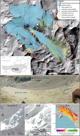


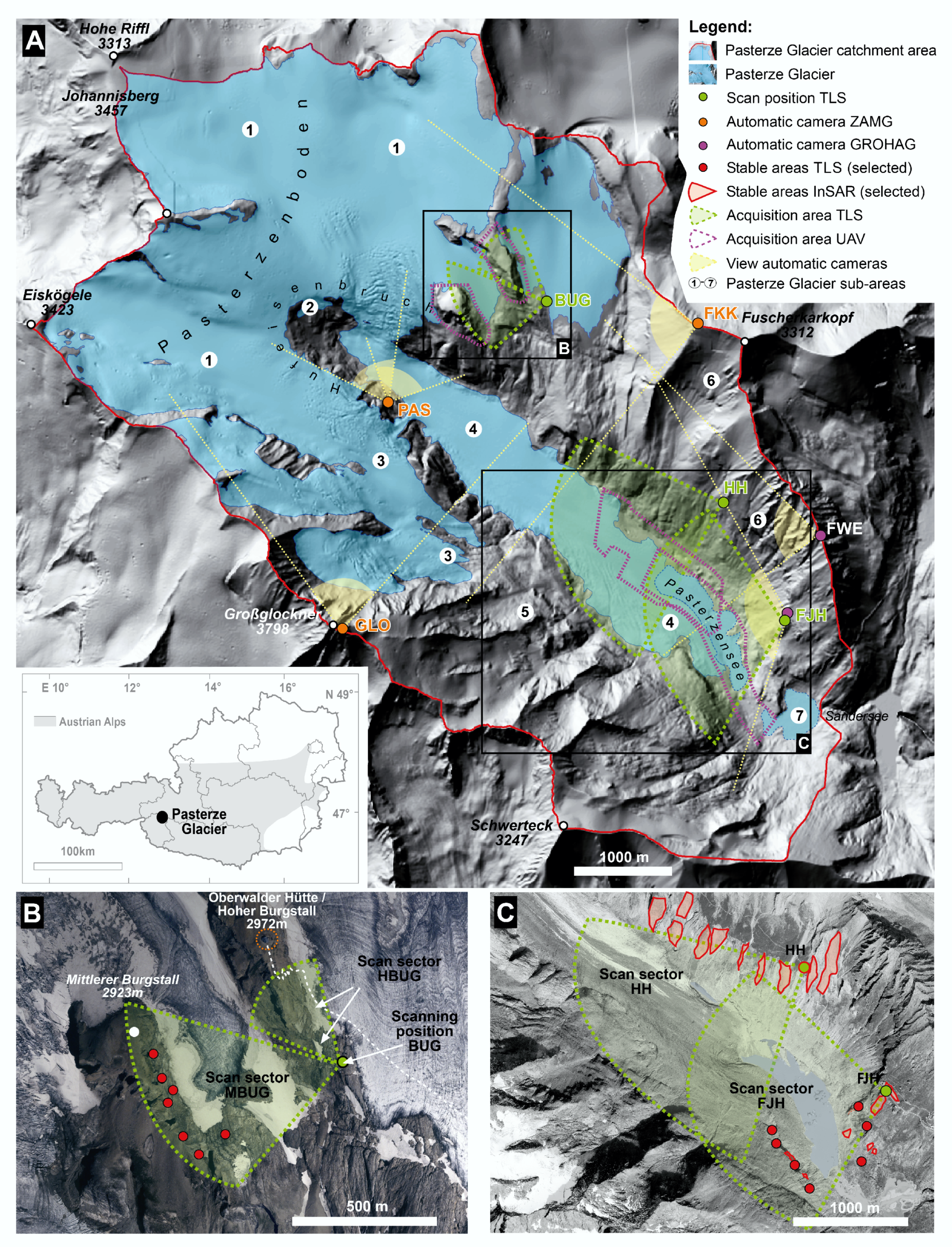
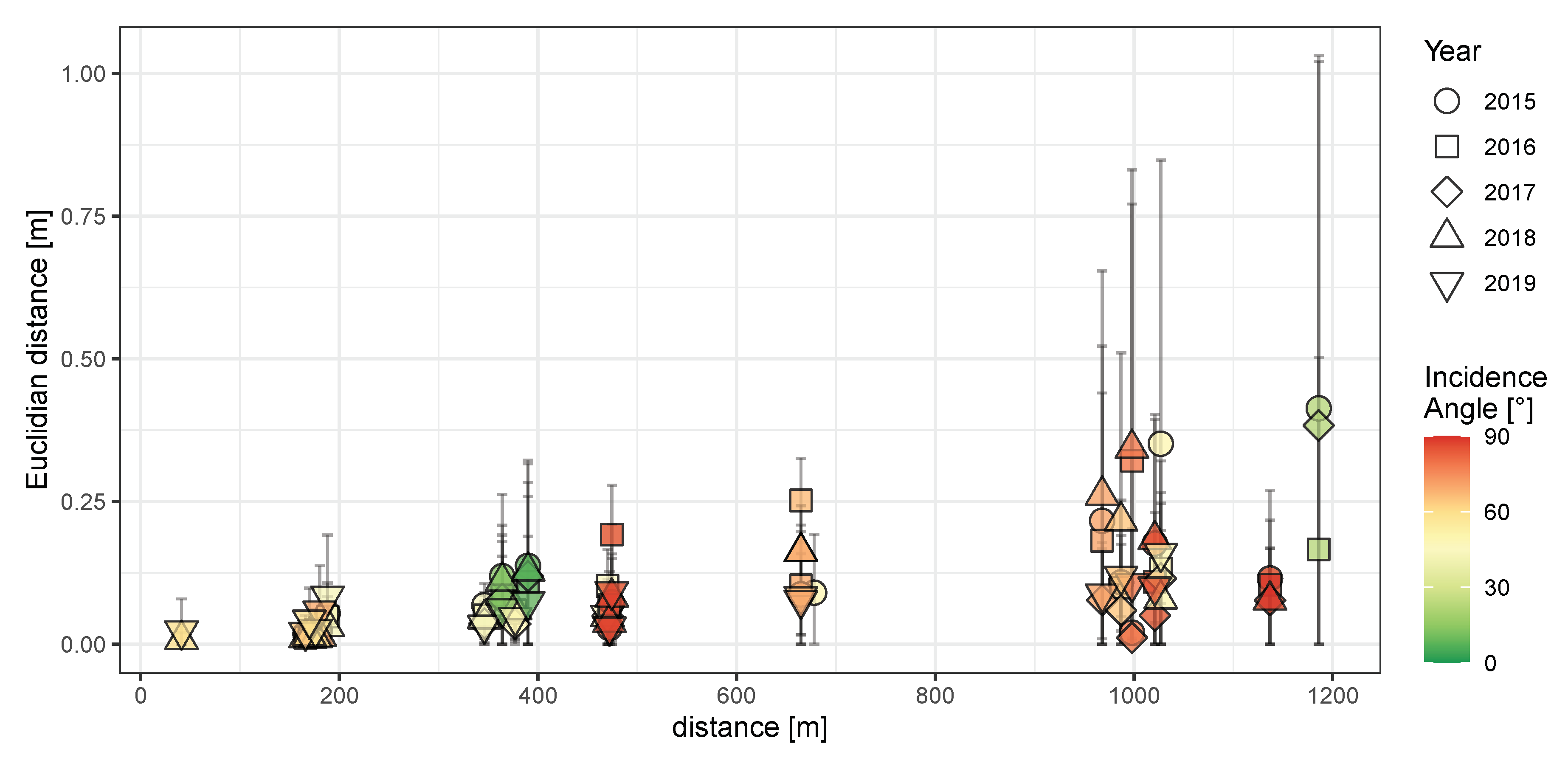
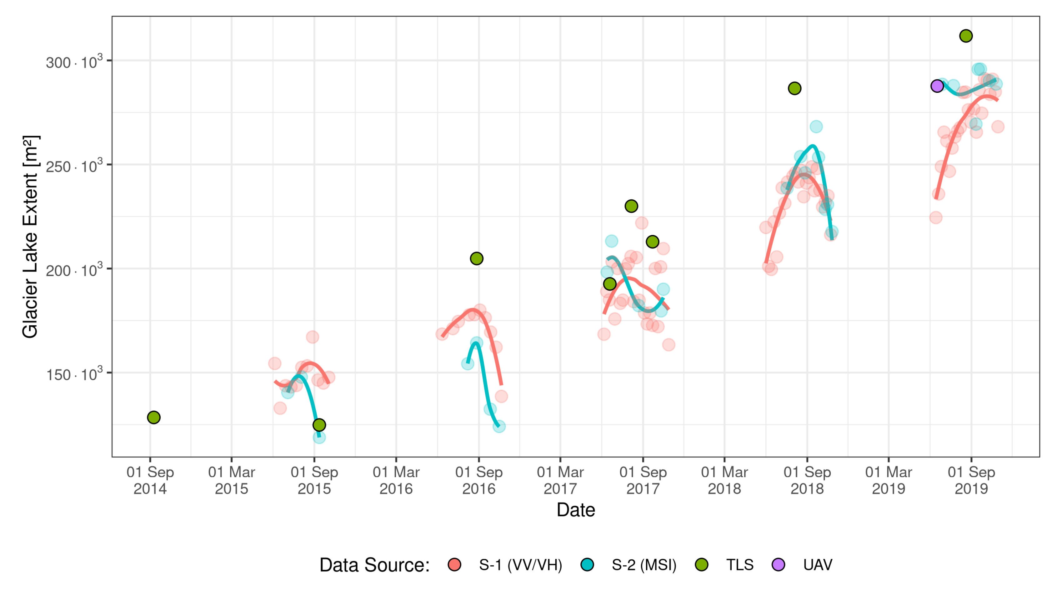
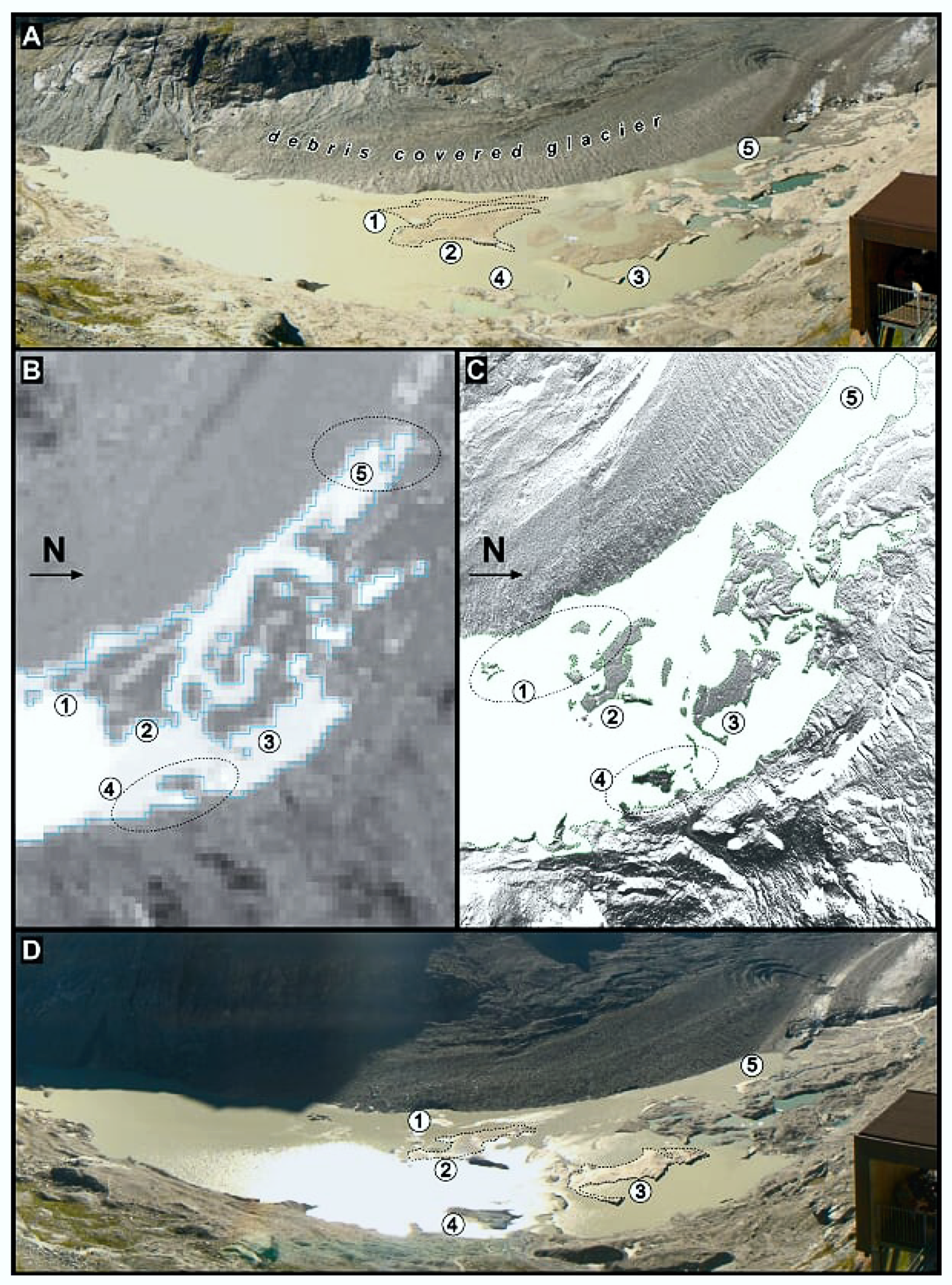
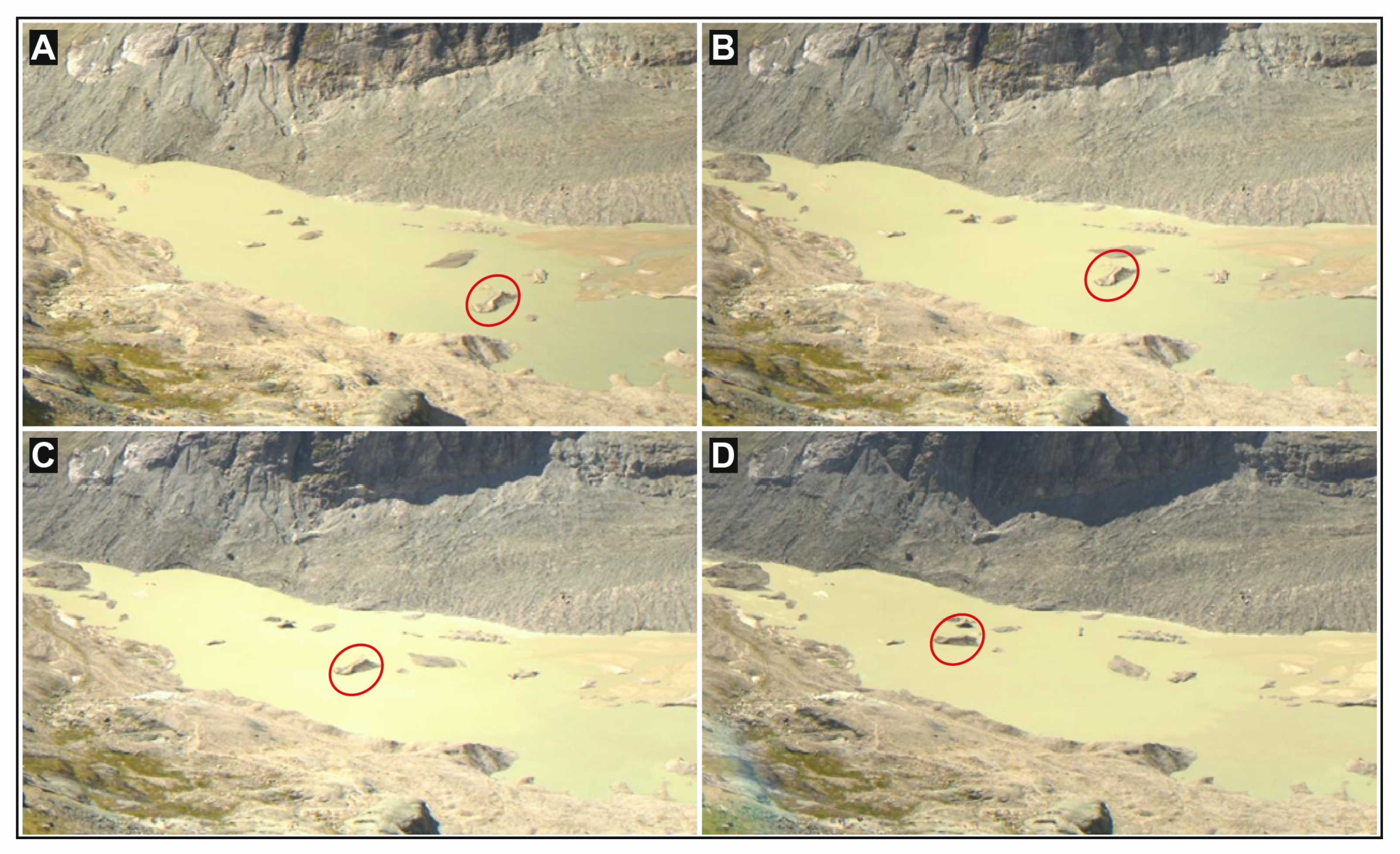
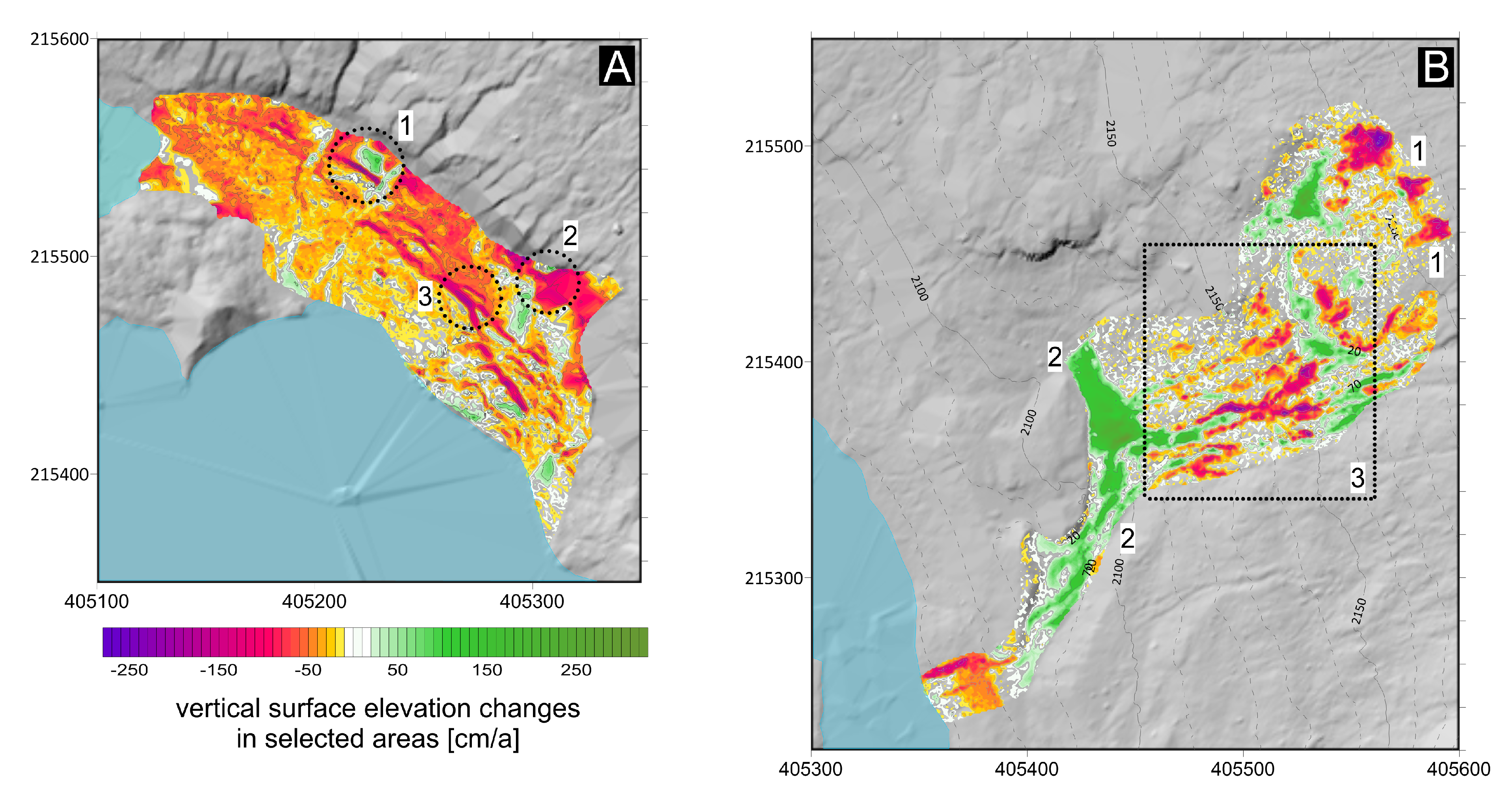
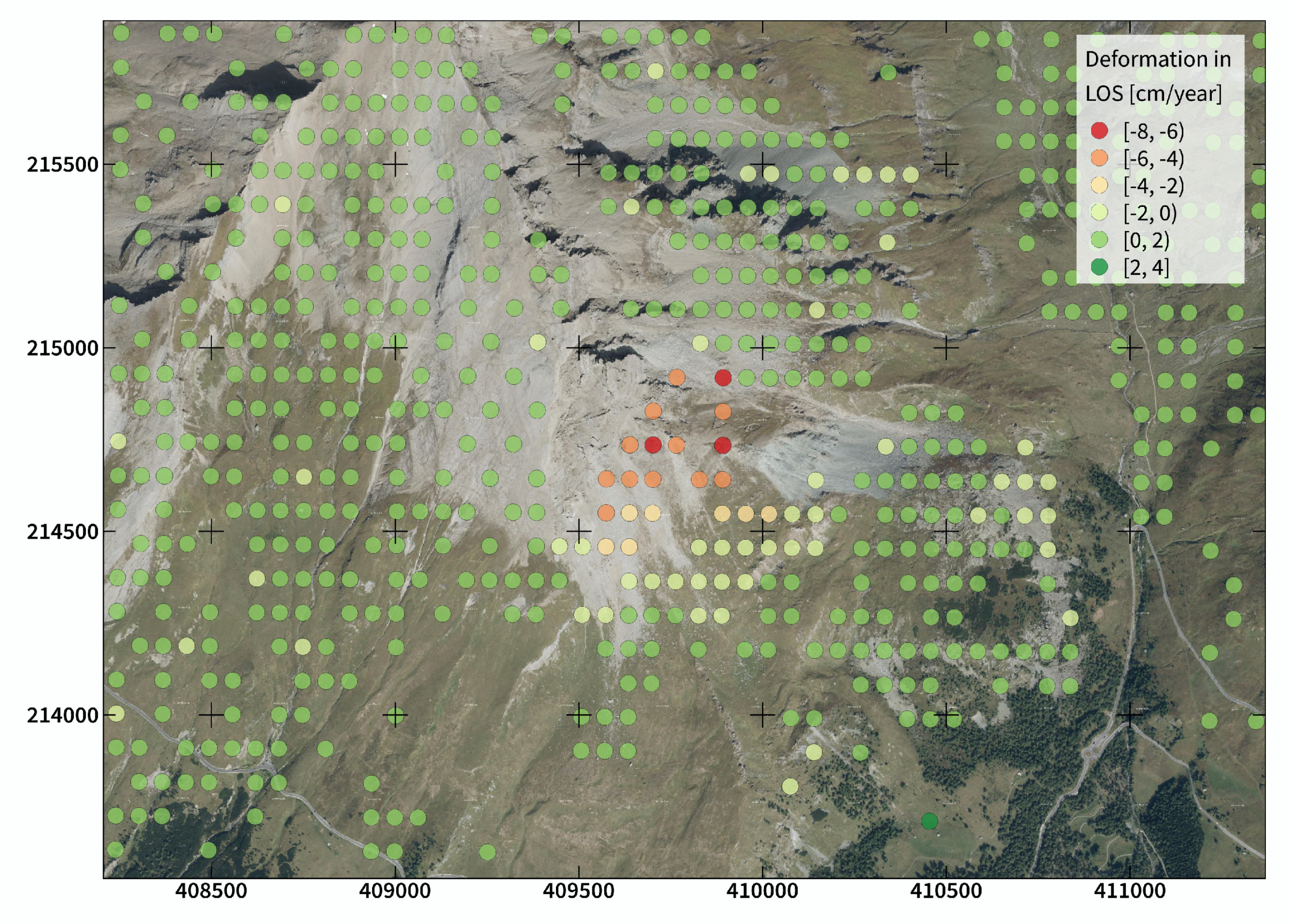