1. Introduction
Arctic sea ice coverage has been monitored since the late 1970s by using remotely sensed sea ice data derived from passive microwave (PM) sensors. A threshold value of 15% sea ice concentration (SIC) has been used traditionally when computing the sea ice extent (SIE) [
1]. This choice of threshold is associated with the accuracy of sea ice concentration retrieval algorithms and based on the studies that the ice extent is well represented by the choice of 15% SIC threshold (e.g., [
2,
3,
4]). On regional scales, ice edges, as observed in satellite data, represented by 5% and 15% thresholds, have been shown to be fairly coherent [
4].
Using synthetic aperture radar (SAR) and ship-based observations, Meier and Notz [
5] have shown that SIC retrieval accuracy can be as poor as ± 20% in summer at the ice edge. The Copernicus Climate Change Service (C3S) uses the ice concentration threshold of 30% to define the ice extent [
6]. Ji et al. [
7] has recommended using 30% as the SIC threshold during summer for SIE calculation based on Special Sensor Microwave Imager/Sounder (SSMIS) data. They also point out the discrepancy in the SIC threshold values used in various ice products.
There are two approaches to defining climatological ice extents using satellite-based SIC data. First, one can define the ice edge using a median edge—defined by the grid cells that have a 50% or higher probability of ice occurring at 15% (or whatever threshold is chosen) concentration or greater for the climate normal period. The climate normal period is defined by World Meteorological Organization (WMO) as the most recent three complete decades, namely, 1981–2010, at the present time. So, using the median approach, at least 15 of these 30 years would need to have ice (above the threshold concentration) to be included in the climatological edge. Alternatively, one can define the ice edge by simply averaging the monthly SIC concentration fields over the 30 years and then thresholding by the defined concentration. Fetterer et al. [
8] argued that the median approach is a more meaningful representation of ice edge compared to the climatological edge because the location of the edge varies considerably from year to year causing the climatological edge to be unlikely to resemble any typical ice edge. The National Snow and Ice Data Center (NSIDC) Sea Ice Index using the median approach is a widely used product for monitoring Arctic sea ice coverage changes [
8].
However, Arctic sea ice loss has accelerated in the last half of the satellite data record (e.g., [
9]) and multi-year ice is depleting faster than ever [
10,
11]. This evolution of these changes brings up a number of scientific questions: Is 15% truly a robust threshold choice to represent sea ice extent decadal trends? Is the remaining sea ice (SIE with SIC of 0–N%, where N% is the SIC threshold) statistically significant to potentially alter the characteristics of distributions? With the potential of the Arctic becoming nearly ice-free, represented by the Arctic sea ice extent falling below 1 mil square kilometers, in the coming decades, what is the sensitivity of the statistical first ice-free Arctic summer year (FIASY) projections to sea ice edge thresholds? Ultimately, the question we strive to answer is: does the choice of threshold have an impact on Arctic sea ice extent decadal trends?
Answering these questions is inhibited by challenges. First, validation data for total sea ice extent is rarely available. Validation of PM sea ice fields is usually done by high-resolution satellite imagery, but these only cover part of the ice cover due to clouds (visible/infrared) [
12] or limited spatial coverage (SAR) [
4,
13]. Secondly, the character of the ice edge can vary widely, even over short distances—from very sharp to very dispersed [
4,
12,
13]. Prior to an extensive investigation, it is beneficial to first examine whether the rapid Arctic sea ice depletion has statistically changed the ice edge characteristics. In this study, we use the National Oceanic and Atmospheric Administration (NOAA)/NSIDC sea ice concentration climate data record to examine how threshold choice may impact the timing of annual SIE minimums and maximums, magnitudes of these extrema, data distributions, and projected FIASY values.
2. Materials and Methods
Monthly sea ice concentration fields from the NOAA and the National Snow and Ice Data Center (NSIDC) Climate Data Record (CDR) [
14] are utilized to derive the monthly sea ice extent time series. The CDR is a long-term, consistent, satellite-based passive microwave record of sea ice concentration [
14]. The CDR product leverages two well-established concentration algorithms, the NASA Team (NT; [
15]) and Bootstrap (BT; [
16]). The NT and BT sea ice concentration algorithms were both developed by the NASA Goddard Space Flight Center (GSFC). Description and verification of the data set can be found in Peng et al. (2013) and Meier et al. (2014), respectively [
17,
18]. The data files used in this study are from the version v03r01 [
14].
The CDR data files include two primary sea ice concentration parameters: the CDR concentration and similar Goddard Merged concentration. Additionally, two GSFC-derived SIC fields are also included in each CDR data file: GSFC-derived NT and BT, respectively. The current CDR concentration spans only from year 1987 to 2017 while the Goddard Merged concentration extends back to 1978. To utilize all the possible satellite data records, we will therefore use the Goddard Merged concentration fields. The Goddard Merged concentration is derived using the same processing algorithm as that for CDR concentration but uses manually quality-controlled GSFC-derived NT and BT sea ice concentrations as input data sources (Meier et al. 2014). Manual quality control means sea ice concentration values may be modified manually at the cell level by examining concentration distributions. The approach is subjective and not reproducible.
The sea ice extent is the area within the contour of a certain concentration threshold,
τ. It is calculated as
where
Ai is the area of pixel
i and
n is the number of pixels. A pixel
i is considered ice covered or not, as defined by
where
SICi is the sea ice concentration of the
ith pixel.
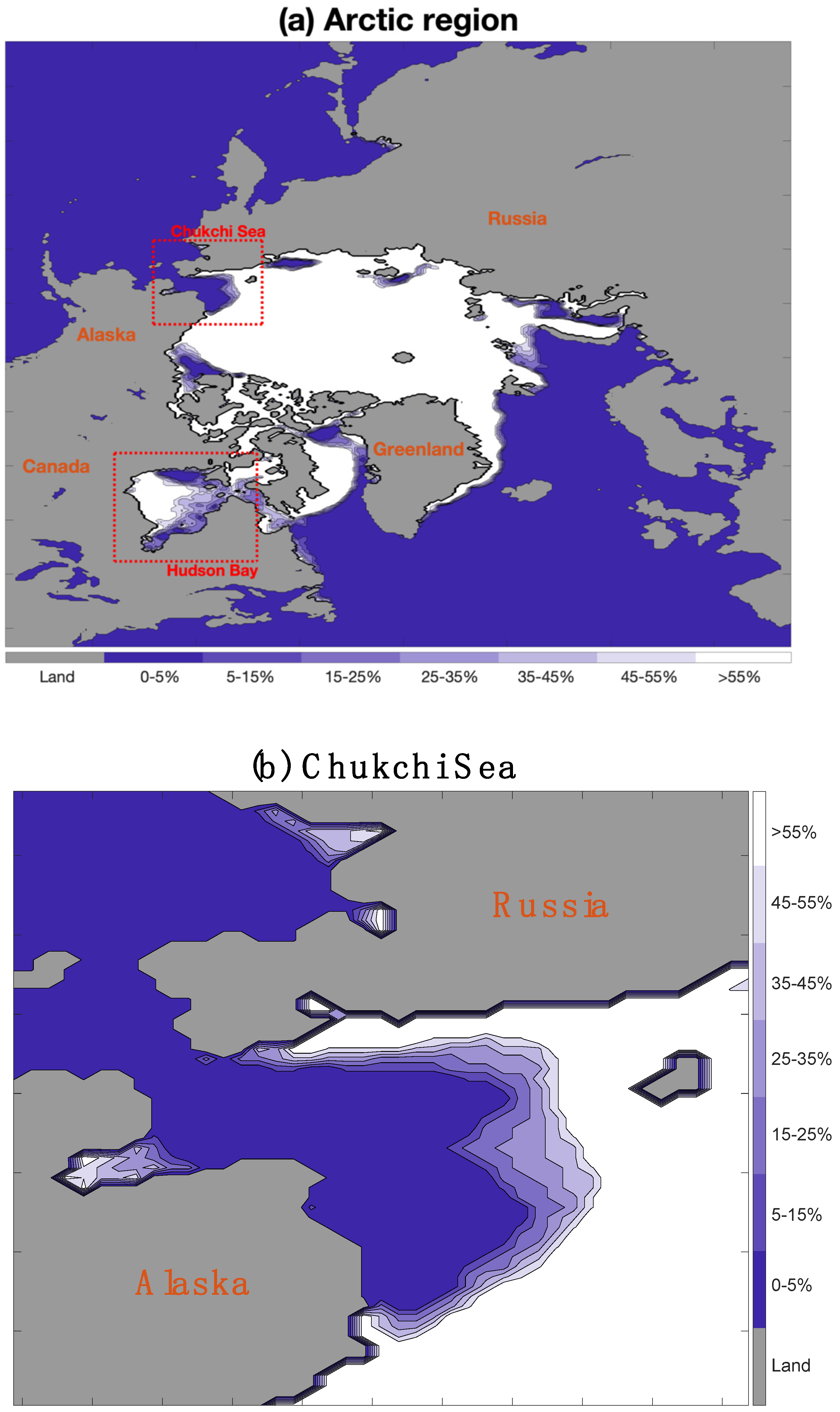
Figure 1 illustrates the impact of the choice of concentration threshold. Here, the
SIC values have been binned to show the potential
SIE contours. The white areas comprise the ice pack with
SIC > 55% while the increasing shades of blue show what additional pixels would be included in the
SIE if lower thresholds were chosen. In
Figure 1a the entire Arctic region is shown, while
Figure 1b zooms into the much-studied Chukchi Sea subregion where it is seen that the contours are fairly coherent in June 2017.
Figure 1c gives a close-up view of the Hudson Bay subregion, where the contours are less coherent, to demonstrate the impact of threshold choice in this situation.
For analysis in this study, the sea ice extent time series has been computed using the sea ice concentration threshold values from 5% to 85% at 5% increments. The sensitivity of the decadal trends of the Arctic sea ice extents to concentration thresholds is examined, as well as that of statistical projections of the FIASY. The FIASY is estimated as the whole number year where the Arctic sea ice extent falls below 1 mil square kilometers. If the projected value falls later than October 1 in the year, the FIASY refers to the following summer.
3. Results
This paper seeks to answer the question: does the choice of threshold have an impact on Arctic annual sea ice extent decadal trends? To address this, a number of supporting analyses are performed. First, we examine the timing of annual SIE minimums and maximums: do they occur in the same month every year, regardless of threshold choice? Then we evaluate the time series of annual SIE minimums and maximums: does threshold choice impact the magnitude of these values? Statistical tests are performed to determine whether data derived from differing thresholds come from the same distributions. Finally, we perform statistical model calibration and selection with data from differing thresholds to determine the impact of threshold choice on optimal model selection along with FIASY estimates.
3.1. Timing of Annual SIE Minimums and Maximums
Using the monthly aggregated time series, annual minimums and maximums were identified along with the month in which those occur.
For thresholds between 5% and 25%, the annual SIE minimum occurs in September for every year analyzed: 1979–2017. For thresholds between 30% and 85%, there is at least one year of the time series where the annual SIE minimum occurs in August. The pattern that this occurs is monotonic, meaning that if a given threshold has the annual minimum in August for a given year, all larger thresholds also have the annual minimum in August. As the threshold increases, this becomes more common to the point where, at the 85% threshold, 24 out of 39 years have an annual minimum in August rather than September.
Behavior for annual maximums is quite different than for annual minimums. For all thresholds and years examined, the maximum always occurs in either February or March. Sometimes as the threshold increases, the annual maximum month switches between February and March (e.g., 1992). Other times, with an increasing threshold, the maximum month switches from March to February (e.g., 1979), but then it may also move oppositely, from February to March (e.g., 1981). These changes in the month of annual maximum can occur with thresholds as low as 5% and 10% (e.g., 1998).
There are several possible reasons why the annual SIE minimum occurs in August rather than September with increasing thresholds. One explanation is temperature based: conditions in September were more conducive for freezing in September rather than continuing to melt. That is, September was colder in that year. As the threshold increases, and data are excluded from the SIE calculation, the magnitude of the SIE value decreases. Because the occurrence of annual SIE minimum in August is only seen in higher thresholds (30–85%), this indicates that less of the ice pack was melting during these years. Freeze up starts in August in the high Arctic, where concentrations stay higher. So, shifting the threshold higher brings the ice edge into higher, colder latitudes, where the concentration begins increasing sooner.
Another explanation is based upon the accuracy of passive microwave SIC retrievals under surface melt conditions. Surface melt results in SIC values that are biased low due to the retrieval algorithms falsely identifying surface pools as open water. With an extreme low SIC bias along with higher threshold values used to calculate SIE, this could result in SIE being biased low as well. The minimum may be shifting to August with increasing thresholds because freeze up has begun in the higher latitude regions, eliminating surface melt and the frequency of low-biased SIC values which exhibited as false annual minimum SIE at the peak of surface melt in August.
3.2. Magnitudes of Annual SIE Minimums and Maximums
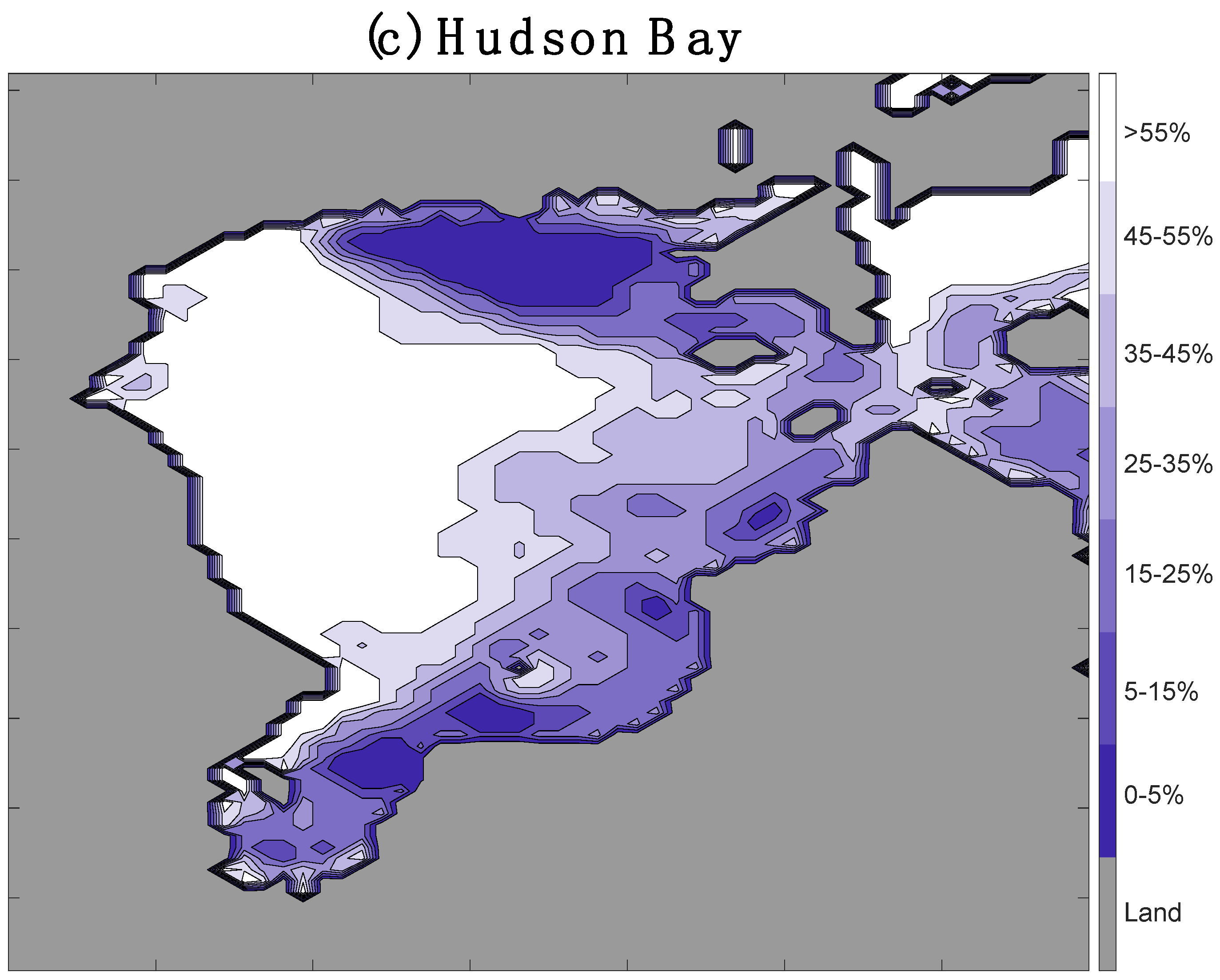
Using the 15% threshold to calculate a baseline SIE annual minimum/maximum time series, we calculate the anomaly as compared to other thresholds. These are presented as percentages in
Figure 2. For example, where SIE_Min
15(t) is the time series of annual SIE minimum time series using the 15% threshold, the anomalies were calculated as
where Y is a different threshold choice.
In
Figure 2a it is seen that reducing the threshold to 5% can increase the annual SIE minimum by up to 4%, while increasing the threshold to 25% will decrease the SIE minimum by potentially 6%. Increasing the threshold to 55% can decrease the SIE minimum by 25%. To a much lesser degree, threshold choice also has an impact on annual SIE maximum values (
Figure 2b). Decreasing the threshold from 15% to 5% leads to between 1% and 2% increase in the annual SIE maximum, while increasing the threshold to 25% may decrease annual SIE maximum by about 2%. Over the course of the available time series, increasing the threshold to 55% can decrease the annual SIE maximum by nearly 9%.
It is valuable to consider whether threshold choice impacts the magnitude of SIE values, and hence the shape of the annual minimum and maximum time series curves, because it can imply that different statistical models may better fit differently shaped curves. There are cases when one threshold choice indicates that the annual minimum is decreasing year over year while another feasible threshold choice indicates that the annual minimum is stable or increasing. For instance, the threshold choice of 10% indicates the annual SIE minimum
increases by 17,221 km
2 between 1986 and 1987, while the threshold choice of 20% indicates it
decreases by 20,040 km
2. This difference in slope indicates that it is possible that different statistical models of the annual SIE minimum time series could be needed depending on the threshold choice used to generate the SIE time series. This will be explored further in
Section 3.4.
3.3. Statistical Comparison of Data Distributions
Two-sample Kolmogorov–Smirnov tests were performed to determine whether data derived from differing thresholds come from the same statistical distributions. The two-sample version of this nonparametric test quantifies the distance between the empirical distribution functions and serves as a useful way to compare two samples as it takes into account differences in both location and shape of the distributions.
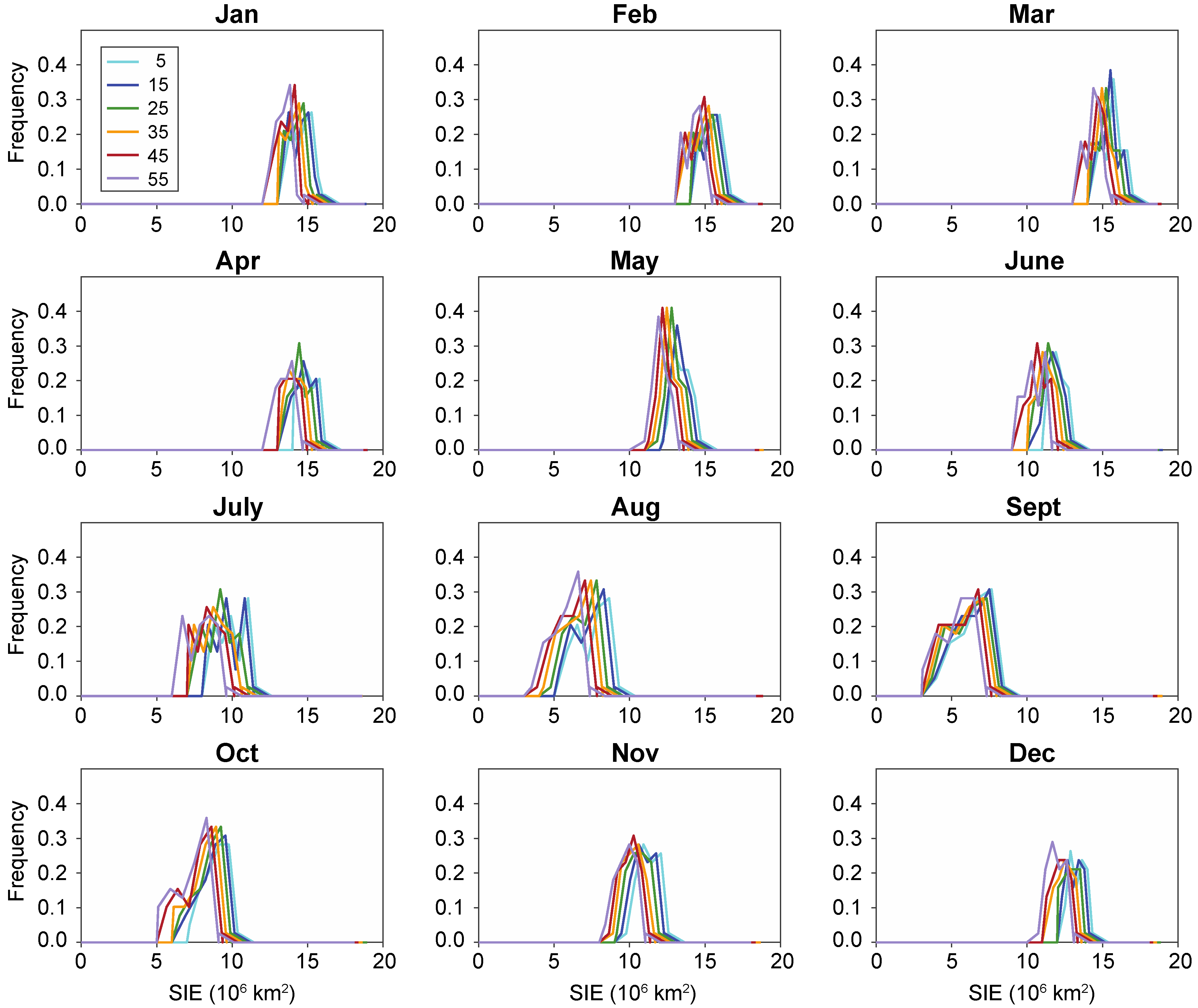
Figure 3 illustrates the shapes of the histograms for a selection of threshold choices (5%, 15%, 25%, 35%, 45%, and 55%). Systematic shifts toward slightly lower sea ice extent values can be seen with increasing thresholds, which is intuitive as fewer cells are included in the extent calculation. Nearly all tests showed similarity in distributions with thresholds within 5% for every month. Some similarities were broader than others, depending on both the threshold choice and month evaluated. As shown in
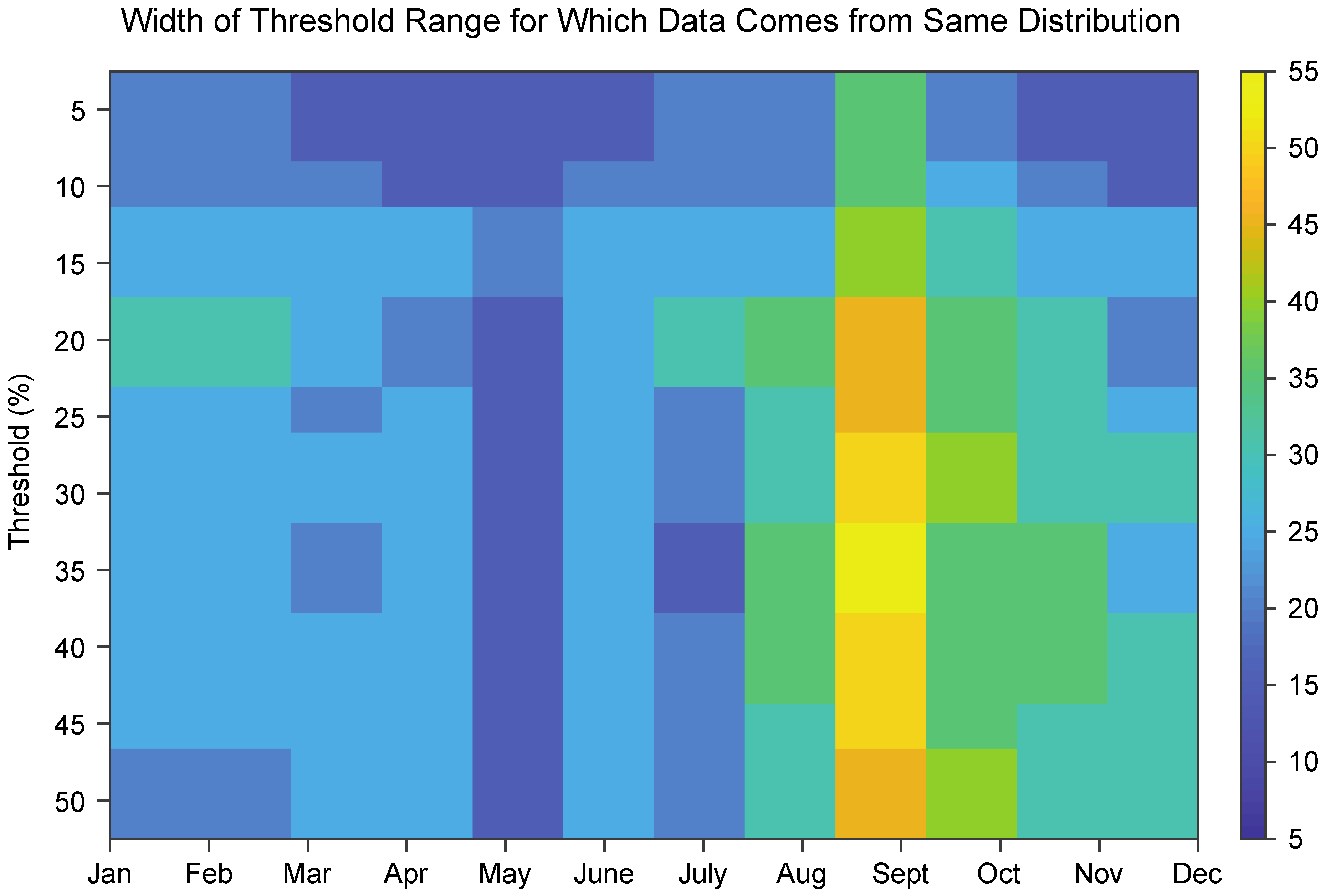
Figure 4, September stands out as a month where the distributions are similar for a wide range of threshold choice, while May has the narrowest band of similarity between distributions for different thresholds.
Table A1 in the
Appendix A lists the details of the threshold values where no significant difference was found between distributions.
There is a strong dependence on seasonality when analyzing whether SIE data, as calculated with different thresholds, come from the same statistical distribution. In September, when annual minimums typically occur, the choice is less critical. Here, a wide range of threshold choices, in fact covering all possible reasonable values as indicated by the literature, yield no significant difference in the distribution of the SIE data. Upon examination of the shapes of the distributions in
Figure 3, this may be attributed to the comparatively large spread of values in September. The lack of importance of threshold choice in September is also consistent with the timing of freeze up, which results in a sharp ice edge pattern as surface melt ceases.
However, the choice of threshold is most critical in May, where changing the threshold by just 10% could yield data with a different distribution shape. A possible explanation here is that at this time the ice is retreating, resulting in variability in the sea outside of the Arctic Ocean. But at the same time there is not yet ice loss within the Arctic Ocean, and thus little variability occurring there.
Figure 3 shows that the shape of the distributions for May are narrowly spread and with sharp peaks in comparison to other months, consistent with the resultant sensitivity to threshold choice.
3.4. Statistical Model Fitting and Selection Using SIE Data with Differing Thresholds
Similar to the analysis done in Peng et al. (2018), where a threshold choice of 15% was used, we perform statistical model calibration and selection with data from SIE annual minimums derived from differing thresholds to determine the impact of threshold choice on optimal model selection along with the FIASY [
19]. Using an updated version of the same long-term, consistent time series of sea ice data, we compare six commonly used statistical models for this type of application. Models are optimized over various segments of the full time series: the first 30 years (1979–2008), all years (1979–2017), and the last 30 years (1988–2017). Following optimization, AICc (Akaike information criterion corrected for small sample size) values are calculated and used to derive the associated W-Akaike weights. The AICc is a statistically-based means of model selection that estimates the quality of each model in comparison to other models for a given data set, taking into account the number of model parameters and data set sample size. Given a set of AICc values, the optimal model of the sample has the minimum value. W-Akaike weights may be interpreted as the probability that the model is the best of the sample. Summing the W-Akaike weights across the sample is 1, and the optimal model of the sample has the maximum (probability) value. The W-Akaike weights are captured in
Table 1.
According to the results in
Table 1, threshold choice does not appear to impact the choice of optimal model from the six examined. Regardless of threshold choice, the exponential model best fits the first 30 years of data, the quadratic model best fits the full time series, and the linear model best fits the last 30 years of data. That said, the probability of these choices does exhibit some change based on threshold choice for several of the fitted domains. In particular, for the full time series (1979–2017) as the threshold is increased the probability of quadratic being the optimal model decreases while the probability of the linear model being optimal increases.
Table 2 summarizes the projected first ice-free Arctic summer year (FIASY) values from all six models over the time period domains of the first 30 years, the full time series, and the last 30 years.
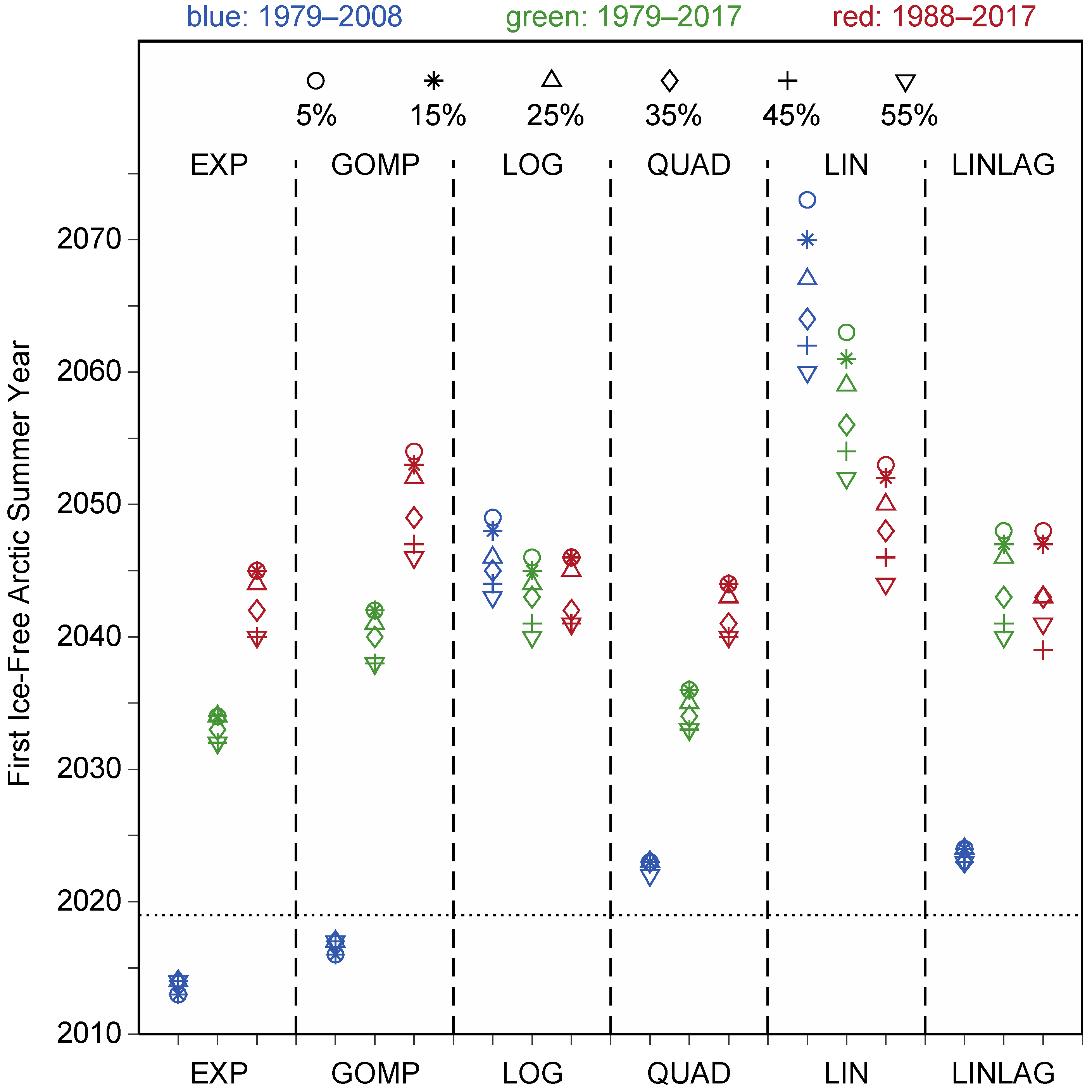
Figure 5 illustrates the impact of threshold, time period domain, and model choice on FIASY predictions. The full results are available in the
Appendix A as
Table A2. In general, increasing the threshold produces an earlier mean modeled FIASY with a slightly smaller spread between model estimates.
In comparison to the similar study done by Peng et al. (2018), where a 15% threshold was used, the models calibrated with the full time series and the last 30 year time periods result in FIASY estimates that are slightly later and with smaller spreads in this analysis. The difference in this paper is that the full time series is 1979–2017, rather than 1979–2015, and the last 30 years is 1988–2017, rather than 1986–2015. The addition of data from 2016 to 2017 appears to be the contributing factor to this change.
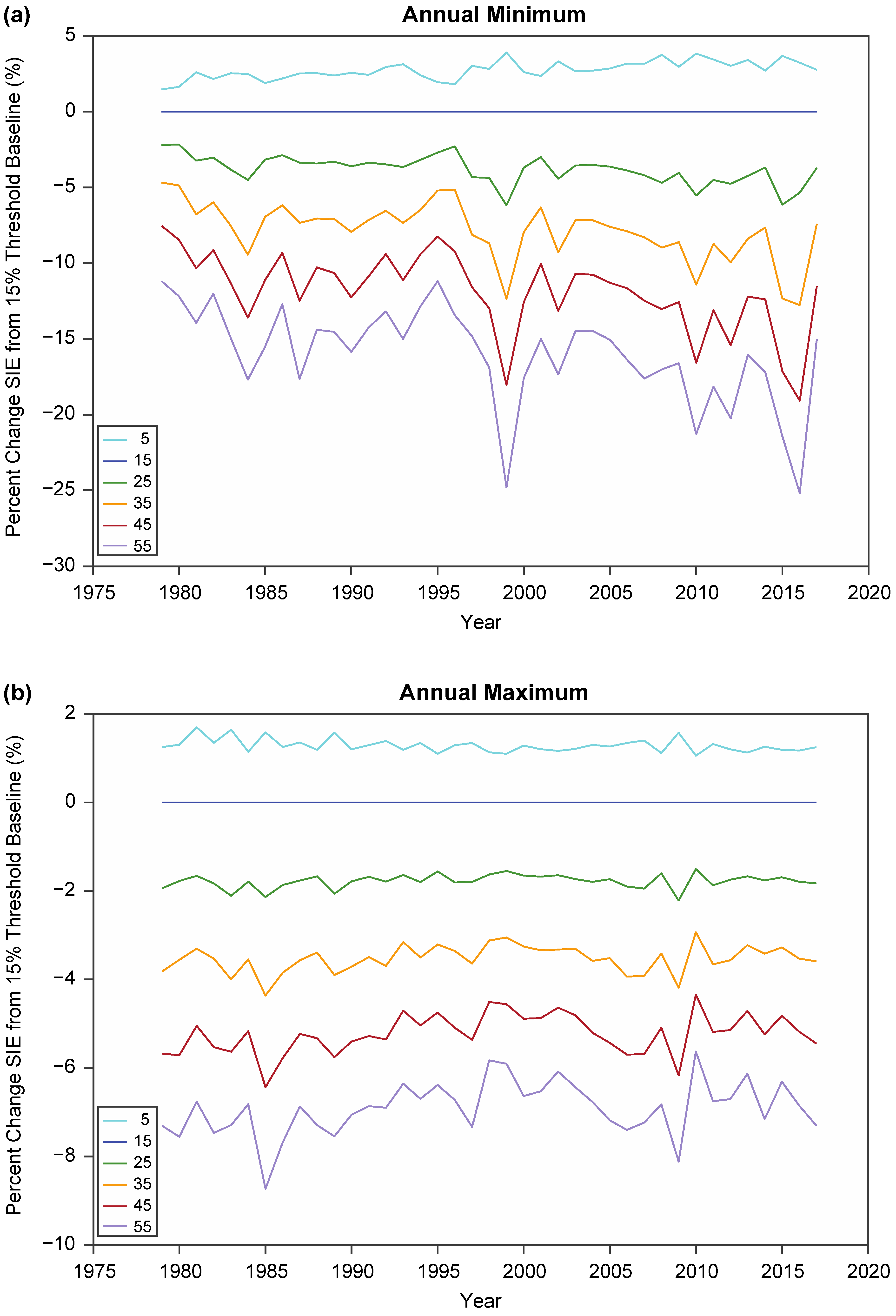
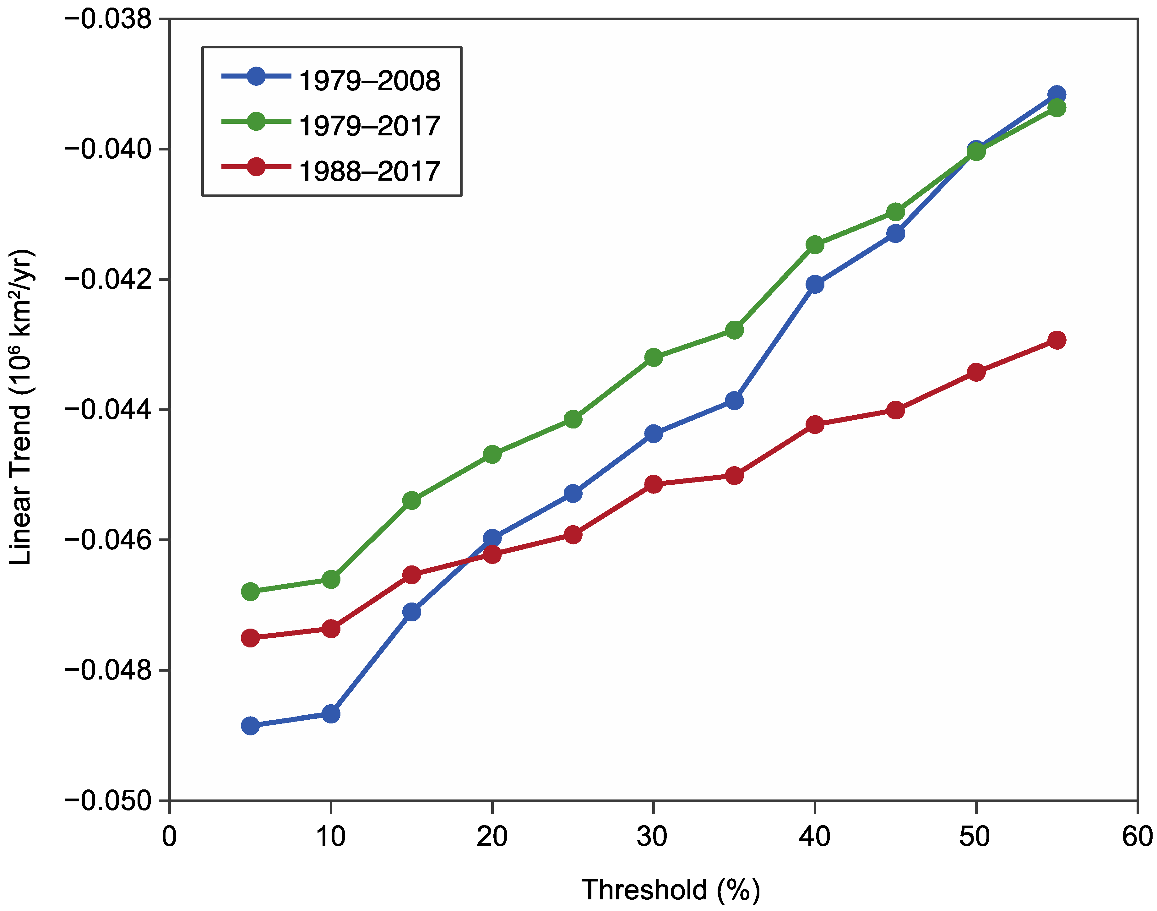
The time series of SIE annual maximums was also examined. Here, the optimal choice of model based on W-Akaike weights was the linear model for every case studied. This includes the three different time domains of calibration, the six different models, and thresholds between 5% and 55%.
Figure 6 shows the fitted linear trends for the different time period domains as a function of threshold. All slopes are negative, as indicated in
Figure 6, meaning that the annual SIE maximum has a decreasing trend for all cases. In general, as the threshold increases, the magnitude of the slope decreases. Thus, using higher thresholds suggests the annual maximum is still decreasing over time, but at a slower rate. The slope magnitude decrease with increasing threshold is more notable when calibrating over the earlier part of the time series. That is, a choice of 55% threshold when fitting over 1979–2008 decreases the magnitude of the slope by 9600 km
2/yr as compared to the 5% threshold. while only 4600 km
2/yr when fitting over the 1988–2017 time period.
3.5. Sensitivity of the FIASY to SIC Threshold
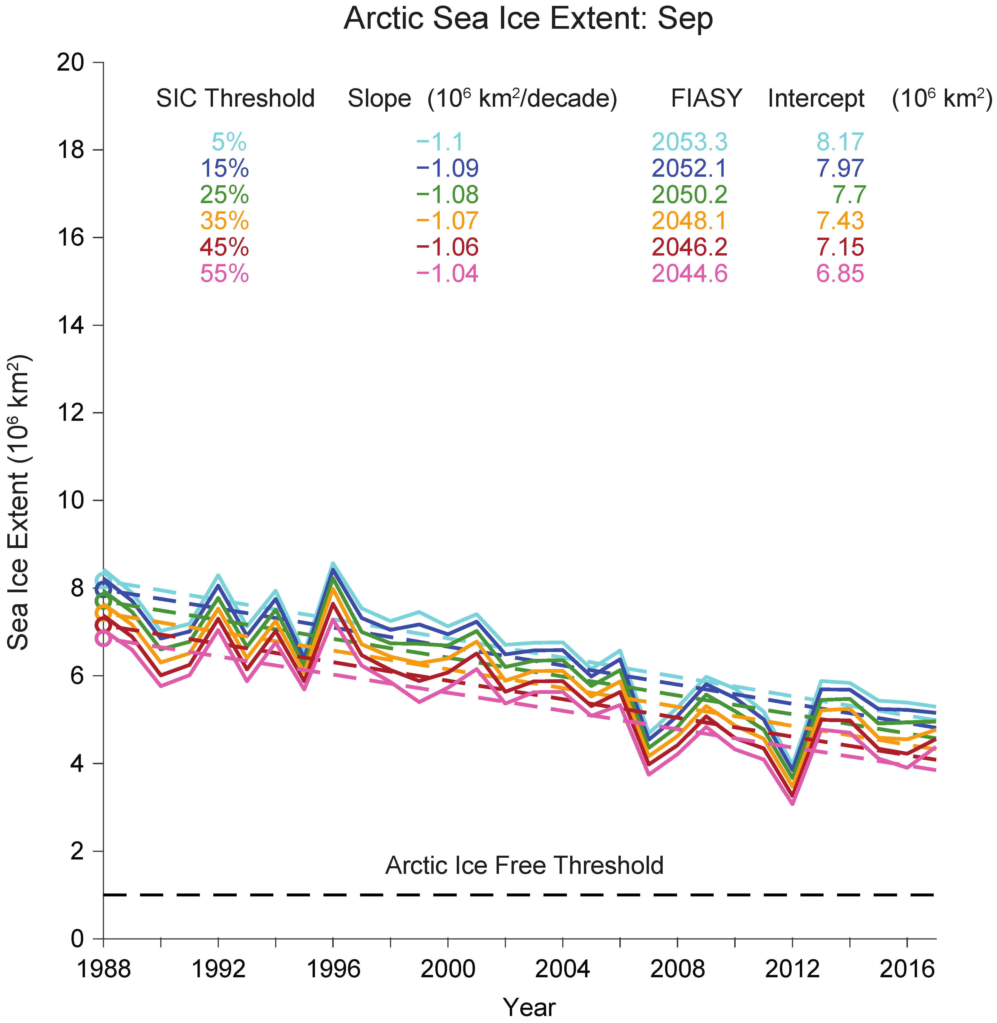
The sensitivity of the FIASY estimates from the linear regression to the SIC thresholds is examined using the SIE times series computed from the SIC threshold values of 5%, 15%, 25%, 35%, 45%, and 55% for the last 30 years (1988–2017). The FIASY value ranges from 2053 for 5% to 2044 for 55%, with a spread of about 7 years (
Figure 7). The downward linear decadal trends of Arctic SIE annual minimum are slightly lower with higher SIC thresholds. Due to the lower initial SIE values, as indicated by the intercept, FIASY values are still relatively earlier, even if with slightly lower trends.
4. Conclusions
The purpose of this study was to answer: does the choice of threshold have an impact on Arctic sea ice extent decadal trends? The answer is yes. We have demonstrated that assuming a threshold choice as low as 30% can impact the timing of SIE annual minimums to occur in August instead of September. The timing of SIE annual maximums is even more sensitive to threshold choice. We have seen that when considering both SIE annual minimum and maximum values, threshold choice is an important factor, more so in the case of minimums where changing the assumed threshold from 15% to 35% could change the magnitude by more than 10%. Monthly SIE data distributions are very seasonally dependent. Although little impact was seen for threshold choice on data distributions during annual minimum times (August and September), there is a strong impact in May.
When evaluating six possible statistical models of annual SIE minimums, threshold choice did not affect optimal model selection; the temporal domain of fitting is the much more significant factor. But, the resultant FIASY estimate is impacted by threshold. Higher threshold choices produce earlier FIASY estimates, and the more notable impact was that FIASY estimates amongst all considered models were more consistent. Furthermore, annual SIE maximums are found to all be decreasing over time regardless of threshold, but the higher thresholds suggest that the long-term trend of decrease is slightly slower.
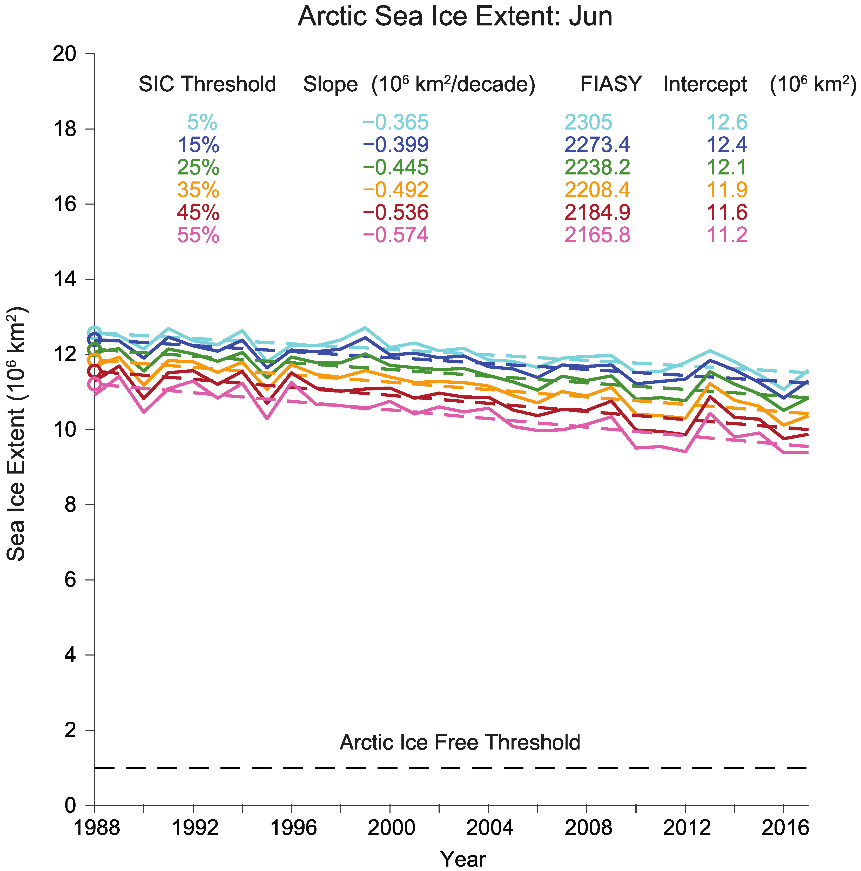
Notably, the impact of surface melt during the peak of melting season has been suggested by this analysis. In
Figure 8, we see that the slopes of the June time series are fairly different between thresholds, as opposed to the September time series, where they were very close to each other (
Figure 7). In September, when SIE is at the annual minimum, it is uniformly cold throughout the region and beginning to freeze, and therefore a surface melt bias is not prominent. However, June is near the peak of the melt season when ice loss is rapidly occurring resulting in more SIC variability near the ice edge. Surface melt is known to impose a negative bias on SIC values, meaning that the presence of surface melt may cause PM SIC retrieval values to be artificially low. Therefore, surface melt could reduce the SIC value to below the threshold used to define SIE. What we see in the June time series is that higher thresholds are exhibiting a faster SIE depletion rate over time, through slopes of higher magnitude. If surface melt is a significant factor that is increasing over time, we would see more cells with lower SIC, meaning that lower thresholds would have an increasingly larger SIE. In turn, this would imply that lower thresholds would have smaller slopes in SIE trends, but artificially so.
In summary, we have validated some obvious outcomes and also uncovered some unexpected impacts of threshold choice on Arctic sea ice extent decadal trends. The more obvious conclusion is that higher thresholds yield lower annual SIE minimums and in turn earlier FIASY estimates. The unexpected outcomes of this threshold choice analysis include evidence about the impact of surface melt. Surface melt is known to bias SIC, and thus SIE, lower. This comes to bear when evaluating the timing of annual SIE minimums, where higher thresholds yield earlier annual minimum dates. Further, during months of peak surface melt (e.g., June) threshold choice has more of an impact on the distribution of SIE values (
Figure 3). And finally, higher thresholds show faster SIE depletion rates during the months of peak surface melt implying that the incidence of surface melt may be increasing in time (
Figure 8).
Given that the rapid Arctic sea ice depletion appears to have statistically changed SIE characteristics, particularly in the summer months, a more extensive investigation to verify surface melt impacts on this data set is warranted. This analysis has suggested that some of the threshold choice impacts to SIE trends may actually be the result of biased data due to surface melt. Until the surface melt is better characterized, and in turn the uncertainty on SIC is better understood, we do not know the true impact of threshold choice to SIE trends as the accuracy of the SIE data itself is in question. Currently, the strongest conclusion that can be made is that certain threshold choices appear to be more sensitive to the impact of surface melt.
Author Contributions
Conceptualization, G.P. and O.B.; methodology, J.L.M and G.P.; software, J.L.M. and G.P.; writing—original draft preparation, J.L.M., with contributions from G.P.; writing—review and editing, J.L.M., G.P., W.N.M., and O.B. All authors have read and agreed to the published version of the manuscript.
Funding
J.L.M., G.P., and O.B. are supported by NOAA’s National Centers for Environmental Information (NCEI) through Cooperative Institute for Climate and Satellites—North Carolina (CICS-NC) under Cooperative Agreement NA14NES432003 and the Cooperative Institute for Satellite Earth System Studies (CISESS) under Cooperative Agreement NA19NES4320002. W.M. is supported by the NASA Earth Science Data and Information System (ESDIS) Project’s Snow and Ice Distributed Active Archive Center (DAAC) at NSIDC under Award Number 80GSFC18C0102.
Conflicts of Interest
The authors declare no conflict of interest. The funders had no role in the design of the study; in the collection, analyses, or interpretation of data; in the writing of the manuscript, or in the decision to publish the results.
Appendix A
Table A1.
Results of the Kolmogorov–Smirnov tests, where entries are the threshold values where no significant difference was found between distributions.
Table A1.
Results of the Kolmogorov–Smirnov tests, where entries are the threshold values where no significant difference was found between distributions.
| Threshold | Jan | Feb | Mar | Apr | May | June | July | Aug | Sept | Oct | Nov | Dec |
|---|
| 5 | 5–20 | 5–20 | 5–15 | 5–15 | 5–15 | 5–15 | 5–20 | 5–20 | 5–35 | 5–20 | 5–15 | 5–15 |
| 10 | 5–20 | 5–20 | 5–20 | 5–15 | 5–15 | 5–20 | 5–20 | 5–20 | 5–35 | 5–25 | 5–20 | 5–15 |
| 15 | 5–25 | 5–25 | 5–25 | 5–25 | 5–20 | 5–25 | 5–25 | 5–25 | 5–40 | 5–30 | 5–25 | 5–25 |
| 20 | 5–30 | 5–30 | 10–30 | 15–30 | 15–25 | 10–30 | 5–30 | 5–35 | 5–45 | 5–35 | 10–35 | 15–30 |
| 25 | 15–35 | 15–35 | 15–30 | 15–35 | 20–30 | 15–35 | 15–30 | 15–40 | 5–45 | 10–40 | 15–40 | 15–35 |
| 30 | 20–40 | 20–40 | 20–40 | 20–40 | 25–35 | 20–40 | 20–35 | 20–45 | 5–50 | 15–50 | 20–45 | 20–45 |
| 35 | 25–45 | 25–45 | 30–45 | 25–45 | 30–40 | 25–45 | 30–40 | 20–50 | 5–55 | 20–50 | 20–50 | 25–45 |
| 40 | 30–50 | 30–50 | 30–50 | 30–50 | 35–45 | 30–50 | 35–50 | 25–55 | 15–60 | 25–55 | 25–55 | 30–55 |
| 45 | 35–55 | 35–55 | 35–55 | 35–55 | 40–50 | 35–55 | 40–55 | 30–55 | 20–65 | 30–60 | 30–55 | 30–55 |
| 50 | 40–55 | 40–55 | 40–60 | 40–60 | 45–55 | 40–60 | 40–55 | 35–60 | 30–70 | 30–65 | 35–60 | 40–65 |
| 55 | 45–60 | 45–60 | 45–65 | 45–65 | 50–65 | 45–65 | 45–60 | 40–65 | 35–70 | 40–65 | 40–65 | 40–65 |
| 60 | 55–65 | 55–65 | 50–70 | 50–70 | 55–70 | 50–70 | 55–65 | 50–70 | 40–75 | 45–70 | 50–70 | 50–75 |
| 65 | 60–70 | 60–70 | 55–70 | 55–75 | 55–70 | 55–70 | 60–70 | 55–75 | 45–80 | 50–75 | 55–75 | 50–75 |
| 70 | 65–75 | 65–75 | 60–75 | 60–75 | 60–75 | 60–75 | 65–75 | 60–75 | 50–85 | 60–80 | 60–80 | 60–80 |
| 75 | 70–80 | 70–80 | 70–80 | 65–80 | 70–75 | 70–80 | 70–80 | 65–80 | 60–85 | 65–85 | 65–85 | 60–80 |
| 80 | 75–85 | 75–85 | 75–85 | 75–85 | 80–85 | 75–80 | 75–85 | 75–85 | 65–85 | 70–85 | 70–85 | 70–85 |
| 85 | 80–85 | 80–85 | 80–85 | 80–85 | 80–85 | 85 | 80–85 | 80–85 | 70–85 | 75–85 | 75–85 | 80–85 |
Table A2.
FIASY estimates for all examined models, time domains of calibration, and thresholds. Entries in bold italics indicate the largest W-Akaike weight values, and hence optimal model, amongst models examined (see weights in
Table 1).
Table A2.
FIASY estimates for all examined models, time domains of calibration, and thresholds. Entries in bold italics indicate the largest W-Akaike weight values, and hence optimal model, amongst models examined (see weights in
Table 1).
| Period | Threshold | Exponential | Gompertz | Log | Quadratic | Linear | Linear w/lag |
|---|
| 1979–1998 (first 20 years) | 5 | 2029 | 2039 | 2084 | 2038 | >2100 | >2100 |
| 15 | 2033 | 2044 | 2083 | 2041 | >2100 | 2048 |
| 25 | 2036 | 2049 | 2086 | 2045 | >2100 | 2051 |
| 35 | 2052 | 2069 | 2070 | 2059 | >2100 | 2064 |
| 45 | 2068 | 2089 | 2082 | 2074 | >2100 | 2084 |
| 55 | >2100 | >2100 | 2088 | >2100 | >2100 | >2100 |
| 1979–2008 (first 30 years) | 5 | 2013 | 2016 | 2049 | 2023 | 2073 | 2024 |
| 15 | 2013 | 2016 | 2048 | 2023 | 2070 | 2024 |
| 25 | 2014 | 2017 | 2046 | 2023 | 2067 | 2024 |
| 35 | 2014 | 2017 | 2045 | 2023 | 2064 | 2023 |
| 45 | 2014 | 2017 | 2044 | 2023 | 2062 | 2023 |
| 55 | 2014 | 2017 | 2043 | 2022 | 2060 | 2023 |
| 1981–2010 (climate normal) | 5 | 2020 | 2024 | 2045 | 2026 | 2064 | 2027 |
| 15 | 2019 | 2024 | 2044 | 2026 | 2062 | 2026 |
| 25 | 2019 | 2023 | 2043 | 2025 | 2060 | 2026 |
| 35 | 2019 | 2023 | 2042 | 2024 | 2057 | 2025 |
| 45 | 2018 | 2022 | 2041 | 2024 | 2056 | 2024 |
| 55 | 2018 | 2022 | 2040 | 2024 | 2054 | 2024 |
| 1979–2017 (all years) | 5 | 2034 | 2042 | 2046 | 2036 | 2063 | 2048 |
| 15 | 2034 | 2042 | 2045 | 2036 | 2061 | 2047 |
| 25 | 2034 | 2041 | 2044 | 2035 | 2059 | 2046 |
| 35 | 2033 | 2040 | 2043 | 2034 | 2056 | 2043 |
| 45 | 2032 | 2038 | 2041 | 2033 | 2054 | 2041 |
| 55 | 2032 | 2038 | 2040 | 2033 | 2052 | 2040 |
| 1988–2017 (last 30 years) | 5 | 2045 | 2054 | 2046 | 2044 | 2053 | 2048 |
| 15 | 2045 | 2053 | 2046 | 2044 | 2052 | 2047 |
| 25 | 2044 | 2052 | 2045 | 2043 | 2050 | 2043 |
| 35 | 2042 | 2049 | 2042 | 2041 | 2048 | 2043 |
| 45 | 2040 | 2047 | 2041 | 2040 | 2046 | 2039 |
| 55 | 2040 | 2046 | 2041 | 2040 | 2044 | 2041 |
| 1998–2017 (last 20 years) | 5 | 2048 | 2088 | 2047 | >2100 | 2048 | >2100 |
| 15 | 2047 | 2086 | 2047 | >2100 | 2047 | >2100 |
| 25 | 2046 | 2083 | 2046 | >2100 | 2046 | >2100 |
| 35 | 2045 | 2079 | 2045 | >2100 | 2045 | >2100 |
| 45 | 2044 | 2076 | 2043 | >2100 | 2044 | 2042 |
| 55 | 2043 | 2074 | 2043 | >2100 | 2043 | 2043 |
References
- Parkinson, C.L.; Comiso, J.C.; Zwally, H.J.; Cavalieri, D.J.; Gloersen, P.; Campbell, W.J. Arctic Sea Ice, 1973–1976: Satellite Passive-Microwave Observations; NASA Goddard Space Flight Center: Greenbelt, MD, USA, 1987.
- Cavalieri, D.J.; Crawford, J.P.; Drinkwater, M.R.; Eppler, D.T.; Farmer, L.D.; Jentz, R.R.; Wacherman, C.C. Aircraft active and passive microwave validation of sea ice concentration from the Defense Meteorological Satellite Program Special Sensor Microwave Imager. J. Geophys. Res. 1991, 96, 21989–22008. [Google Scholar] [CrossRef]
- Gloersen, P.; Campbell, W.J.; Cavalieri, D.J.; Comiso, J.C.; Parkinson, C.L.; Zwally, H.J. Arctic and Antarctic Sea Ice, 1978–1987: Satellite Passive-Microwave Observations and Analysis; NASA SP-511; NASA Headquarters: Washington, DC, USA, 1992; p. 306.
- Meier, W.N.; Maksym, T.; Van Woert, M.L. Evaluation of Arctic operational passive microwave products: A case study in the Barents Sea during October 2001. In Proceedings of the Ice in the Environment: Proceedings of the 16th IAHR International Symposium on Ice, Dunedin, New Zealand, 2–6 December 2003. [Google Scholar]
- Meier, W.N.; Notz, D. A note on the accuracy and reliability of satellite-derived passive microwave estimates of sea-ice extent. In Proceedings of the CliC Arctic sea ice working group consensus document, World Climate Research Program, Tromsø, Norway, 28 October 2010. [Google Scholar]
- Aaboe, S.; Sørensen, A.; Lavergne, T.; Eastwood, S. Algorithm Theoretical Basis Document—Sea Ice Edge and Sea Ice Type Climate Data Records; Copernicus Climate Change Service 25/05/2018; Copernicus Climate Change Service: Reading, UK, 2018; p. 26. [Google Scholar]
- Ji, Q.; Li, F.; Pang, X.; Luo, C. Statistical analysis of SSMIS sea ice concentration threshold at the Arctic Sea Ice Edge during summer based on MODIS and ship-based observational data. Sensors 2018, 18, 1109. [Google Scholar] [CrossRef] [PubMed] [Green Version]
- Fetterer, F.; Knowles, K.; Meier, W.N.; Savoie, M.M.; Windnagel, A.K. Sea Ice Index, Version 3, Updated Daily; National Snow and Ice Data Center: Boulder, CO, USA, 2017. [CrossRef]
- Peng, G.; Meier, W.N. Temporal and regional variability of Arctic sea-ice coverage from satellite data. Ann. Glaciol. 2017, 59, 191–200. [Google Scholar] [CrossRef] [Green Version]
- Kwok, R.; Untersteiner, N. The thinning of Arctic sea ice. Phys. Today 2011, 64, 36–41. [Google Scholar] [CrossRef] [Green Version]
- Comiso, J.J. Large decadal decline of the arctic multiyear ice cover. J. Clim. 2012, 25, 1176–1193. [Google Scholar] [CrossRef]
- Meier, W.N. Comparison of passive microwave ice concentration algorithm retrievals with AVHRR imagery in the Arctic peripheral seas. IEEE Trans. Geosci. Rem. Sens. 2005, 43, 1324–1337. [Google Scholar] [CrossRef]
- Heinrichs, J.F.; Cavalieri, D.J.; Markus, T. Assessment of the AMSR-E sea ice concentration product at the ice edge using RADARSAT-1 and MODIS imagery. IEEE Trans. Geosci. Rem. Sens. 2006, 44, 3070–3080. [Google Scholar] [CrossRef]
- Meier, W.N.; Fetterer, F.; Savoie, M.; Mallory, S.; Duerr, R.; Stroeve, J. NOAA/NSIDC Climate Data Record of Passive Microwave Sea Ice Concentration, Version 3; National Snow and Ice Data Center: Boulder, CO, USA, 2017. [CrossRef]
- Cavalieri, D.J.; Parkinson, C.L.; Gloersen, P.; Zwally, H.J. Sea Ice Concentrations from Nimbus-7 SMMR and DMSP SSM/I-SSMIS Passive Microwave Data, Version 1; NASA National Snow and Ice Data Center Distributed Active Archive Center: Boulder, CO, USA, 1996. [CrossRef]
- Comiso, J.C. Bootstrap Sea Ice Concentrations from Nimbus-7 SMMR and DMSP SSM/I-SSMIS, Version 3; NASA National Snow and Ice Data Center Distributed Active Archive Center: Boulder, CO, USA, 2017. [CrossRef]
- Peng, G.; Meier, W.N.; Scott, D.J.; Savoie, M. A long-term and reproducible passive microwave sea ice concentration data record for climate studies and monitoring. Earth-Syst. Sci. Data 2013, 5, 311–318. [Google Scholar] [CrossRef] [Green Version]
- Meier, W.N.; Peng, G.; Scott, D.J.; Savoie, M.H. Verification of a new NOAA/NSIDC passive microwave sea-ice concentration climate record. Polar Res. 2014, 33. [Google Scholar] [CrossRef] [Green Version]
- Peng, G.; Matthews, J.L.; Yu, J.T. Sensitivity analysis of Arctic sea ice extent trends and statistical projections using satellite data. Remote Sens. 2018, 10, 230. [Google Scholar] [CrossRef] [Green Version]
Figure 1.
Binned June 2017 sea ice concentration (SIC) observations for the (a) Arctic region, (b) Chukchi Sea, and (c) Hudson Bay. The upper red dashed box in (a) indicates the Chukchi Sea subregion displayed in (b) and the lower red dashed box highlights the Hudson Bay subregion displayed in (c).
Figure 1.
Binned June 2017 sea ice concentration (SIC) observations for the (a) Arctic region, (b) Chukchi Sea, and (c) Hudson Bay. The upper red dashed box in (a) indicates the Chukchi Sea subregion displayed in (b) and the lower red dashed box highlights the Hudson Bay subregion displayed in (c).
Figure 2.
Percent change in sea ice extent (SIE) with varying threshold choices as compared to SIE calculated with the 15% threshold for annual SIE (a) minimums and (b) maximums.
Figure 2.
Percent change in sea ice extent (SIE) with varying threshold choices as compared to SIE calculated with the 15% threshold for annual SIE (a) minimums and (b) maximums.
Figure 3.
Histograms of SIE over the 1979–2017 time period by month for different concentration thresholds (colored lines, in %).
Figure 3.
Histograms of SIE over the 1979–2017 time period by month for different concentration thresholds (colored lines, in %).
Figure 4.
The width of the threshold range for which data comes from the same distribution, as evaluated by two-sample Kolmogorov–Smirnov tests, both as a function of month and threshold. For example, when looking at May, the distribution of SIE values resulting from a 10% threshold choice is not significantly different from distributions of SIE values resulting from 5% or 15% threshold choices. Thus, the width of the range for which data comes from the same distribution is 10.
Figure 5.
The projected FIASY from six different statistical models (organized as columns) where color depicts the temporal domain of model calibration, and symbol indicates the threshold choice. The dashed line indicates the present year, so it may be interpreted that predictions under this line are infeasible.
Figure 6.
Optimized slopes of linear regression fits to the SIE annual maximum time series.
Figure 6.
Optimized slopes of linear regression fits to the SIE annual maximum time series.
Figure 7.
Arctic annual minimum SIE time series (solid) for 1988–2017 and their linear regressions (dashed) for varying SIC thresholds. The circles represent the initial positions (the 1988 value of the trend line) of the linear regression (Intercept).
Figure 7.
Arctic annual minimum SIE time series (solid) for 1988–2017 and their linear regressions (dashed) for varying SIC thresholds. The circles represent the initial positions (the 1988 value of the trend line) of the linear regression (Intercept).
Figure 8.
Arctic June monthly SIE time series (solid) for 1988–2017 and their linear regressions (dashed) for varying SIC thresholds.
Figure 8.
Arctic June monthly SIE time series (solid) for 1988–2017 and their linear regressions (dashed) for varying SIC thresholds.
Table 1.
W-Akaike weights [unitless] as calculated from Akaike information criterion corrected (AICc) values for models of annual SIE minimums. Entries in bold italics indicate the largest value, and hence optimal model, amongst models examined.
Table 1.
W-Akaike weights [unitless] as calculated from Akaike information criterion corrected (AICc) values for models of annual SIE minimums. Entries in bold italics indicate the largest value, and hence optimal model, amongst models examined.
| Period | Threshold | Exponential | Gompertz | Log | Quadratic | Linear | Linear w/lag |
|---|
| 1979–2008 (first 30 years) | 5 | 0.48 | 0.42 | 0.0009 | 0.094 | 0.0015 | 0.0053 |
| 15 | 0.49 | 0.41 | 0.00098 | 0.092 | 0.0016 | 0.0052 |
| 25 | 0.49 | 0.41 | 0.0015 | 0.099 | 0.0026 | 0.0056 |
| 35 | 0.48 | 0.40 | 0.0026 | 0.11 | 0.0044 | 0.0062 |
| 45 | 0.47 | 0.39 | 0.0038 | 0.12 | 0.0067 | 0.0068 |
| 55 | 0.46 | 0.38 | 0.0051 | 0.14 | 0.0089 | 0.0078 |
| 1979–2017 (all years) | 5 | 0.19 | 0.26 | 0.069 | 0.32 | 0.086 | 0.076 |
| 15 | 0.19 | 0.26 | 0.077 | 0.31 | 0.099 | 0.068 |
| 25 | 0.19 | 0.26 | 0.084 | 0.30 | 0.11 | 0.057 |
| 35 | 0.19 | 0.27 | 0.085 | 0.29 | 0.11 | 0.047 |
| 45 | 0.20 | 0.28 | 0.084 | 0.29 | 0.11 | 0.042 |
| 55 | 0.20 | 0.27 | 0.091 | 0.28 | 0.12 | 0.040 |
| 1988–2017 (last 30 years) | 5 | 0.13 | 0.14 | 0.13 | 0.14 | 0.44 | 0.011 |
| 15 | 0.13 | 0.14 | 0.13 | 0.13 | 0.44 | 0.011 |
| 25 | 0.13 | 0.14 | 0.13 | 0.13 | 0.45 | 0.0083 |
| 35 | 0.13 | 0.15 | 0.13 | 0.13 | 0.44 | 0.011 |
| 45 | 0.13 | 0.15 | 0.13 | 0.14 | 0.44 | 0.0084 |
| 55 | 0.13 | 0.15 | 0.13 | 0.13 | 0.45 | 0.011 |
Table 2.
Metrics from six model projections of first ice-free Arctic summer year (FIASY). Minimum, mean, and maximum are calculated as described in the methods. The standard deviation is rounded to the nearest whole number.
Table 2.
Metrics from six model projections of first ice-free Arctic summer year (FIASY). Minimum, mean, and maximum are calculated as described in the methods. The standard deviation is rounded to the nearest whole number.
| Years | Threshold | Minimum | Mean | Maximum | Std. Dev. |
|---|
| 1979–2008 | 5 | 2013 | 2033 | 2073 | 23 |
| 15 | 2013 | 2032 | 2070 | 22 |
| 25 | 2014 | 2032 | 2067 | 21 |
| 35 | 2014 | 2031 | 2064 | 19 |
| 45 | 2014 | 2030 | 2062 | 19 |
| 55 | 2014 | 2030 | 2060 | 18 |
| 1979–2017 | 5 | 2034 | 2045 | 2063 | 10 |
| 15 | 2034 | 2044 | 2061 | 10 |
| 25 | 2034 | 2043 | 2059 | 9 |
| 35 | 2033 | 2041 | 2056 | 8 |
| 45 | 2032 | 2040 | 2054 | 8 |
| 55 | 2032 | 2039 | 2052 | 7 |
| 1988–2017 | 5 | 2044 | 2048 | 2054 | 4 |
| 15 | 2044 | 2048 | 2053 | 4 |
| 25 | 2043 | 2046 | 2052 | 4 |
| 35 | 2041 | 2044 | 2049 | 3 |
| 45 | 2039 | 2042 | 2047 | 3 |
| 55 | 2040 | 2042 | 2046 | 2 |
© 2020 by the authors. Licensee MDPI, Basel, Switzerland. This article is an open access article distributed under the terms and conditions of the Creative Commons Attribution (CC BY) license (http://creativecommons.org/licenses/by/4.0/).


