Article

Impact of Sea Breeze Dynamics on Atmospheric Pollutants and Their Toxicity in Industrial and Urban Coastal Environments

1
Univ. Littoral Côte d’Opale, UR 4493—LPCA—Laboratoire de Physico-Chimie de l’Atmosphère, 59140 Dunkerque, France
2
Univ. Littoral Côte d’Opale, SFR Condorcet FR CNRS 3417, UR 4492—UCEiV—Unité de Chimie Environnementale et Interactions sur le Vivant, 59140 Dunkerque, France
3
Univ. Lille, CNRS, UMR 8518—LOA—Laboratoire d’Optique Atmosphérique, 59000 Lille, France
4
Univ. Lille, CNRS, UMR 8522—PC2A—Physico-Chimie des Processus de Combustion et de l’Atmosphère, 59000 Lille, France
5
Univ. Lille, Univ. Littoral Côte d’Opale, CNRS, UMR 8187—LOG—Laboratoire d’Océanologie et de Géosciences, F 62930 Wimereux, France
*
Author to whom correspondence should be addressed.
Remote Sens. 2020, 12(4), 648; https://doi.org/10.3390/rs12040648
Submission received: 16 January 2020 / Revised: 11 February 2020 / Accepted: 13 February 2020 / Published: 15 February 2020
(This article belongs to the Special Issue Lidar Remote Sensing of Aerosols Observation)

Abstract

:
Sea breeze (SB) phenomena may strongly influence air quality and lead to important effects on human health. In order to study the impact of SB dynamics on the properties and toxicity of aerosols, an atmospheric mobile unit was deployed during a field campaign performed in an urbanized and industrialized coastal area in Northern France. This unit combines aerosol samplers, two scanning lidars (Doppler and elastic) and an air-liquid interface (ALI, Vitrocell®) in vitro cell exposure device. Our study highlights that after the passage of an SB front, the top of the atmospheric boundary layer collapses as the thermal internal boundary layer (TIBL) develops, which leads to high aerosol extinction coefficient values (>0.4 km−1) and an increase of PM2.5 and NOx concentrations in the SB current. The number-size distribution of particles indicates a high proportion of fine particles (with diameter below 500 nm), while the volume-size distribution shows a major mode of coarse particles centered on 2–3 µm. Individual particle analyses performed by cryo-transmission scanning electron microscopy (cryo-TSEM)-EDX highlights that submicronic particles contained a high fraction of secondary compounds, which may result from nucleation and/or condensation of condensable species (vapors or gaseous species after photo-oxidation). Secondary aerosol (SA) formation can be enhanced in some areas, by the interaction between the SB flow and the upper continental air mass, particularly due to the effect of both turbulence and temperature/humidity gradients between these two contrasting air masses. Potential areas of SA formation are located near the ground, during the SB front passage and in the vicinity of the SB current top. During the sea breeze event, an increase in the oxidative stress and inflammation processes in exposed lung cells, compared to the unexposed cells, can also be seen. In some instances, short singularity periods are observed during SB, corresponding to a double flow structure. It consists of two adjacent SB currents that induce an important increase of the TIBL top, improving the pollutants dispersion. This is associated with a substantial decrease of aerosol mass concentrations.

Graphical Abstract

1. Introduction

Atmospheric aerosol properties are greatly dependent on their sources and vary geographically as a function of processing and transport, mostly driven by meteorological conditions. Coastal industrial and urban areas are frequently subject to mediocre air quality episodes, mainly due to local meteorological phenomena affecting pollutant dispersion [1]. Moreover, the large diversity of pollutant sources, in such a multi-influenced environment, associated with the dynamics of the atmosphere, may give rise to a large number of aerosol plumes, with widely variable properties. As these properties evolve quickly within the atmosphere [2], it is important to better understand the local meteorological phenomena, along with a parallel characterization of aerosol particles, to assess, for instance, their effects on human health [3,4,5,6]. More generally, the size and chemical composition of anthropogenic and natural particles influence aerosol optical properties and subsequently their ability to interact with solar radiation [7]. In this regard, particle size is a crucial parameter in aerosol climate interactions, via its direct radiative effects or via its indirect effects, such as altering cloud properties (cloud droplet size, concentration, cloud extinction) [8].
Sea breeze (SB) is a mesoscale meteorological phenomenon which has a significant influence on coastal air quality through its ability to efficiently mix different aerosol types and condensable gases, and, therefore, to favor the formation of secondary products or to enhance coagulation processes [9,10,11,12]. SB can drive the dispersion of pollutants and their evolution by ventilation, stagnation, recirculation, gravity current transport processes, and by the evolution of the thermal internal boundary layer (TIBL) structure, corresponding to the local atmospheric boundary layer (ABL) [13,14]. SB associated with a complex array of emission sources may deeply modify the aerosol size distribution, composition, and their vertical profile, which will imply differences in their impact on radiative properties [15]. Hence, all these processes may contribute to the variability and complexity of the atmospheric dynamics structure and to the temporal variations of aerosol concentrations in coastal regions. Fine particles (diameter < 1 µm) represent the vast majority of the total aerosol number concentration which may have some effect on human health [16,17]. Depending on their physical and chemical properties, these particles can penetrate deeply into the human lung via inhalation and most of them will be deposited within the lungs, leading to respiratory diseases [18,19,20].
While many studies have been devoted to better understand the potential role of SB activity on distribution of pollutants [21,22,23,24,25] or the association of fine particle exposure with acute respiratory inflammation [26,27], only few studies have focused on fine spatiotemporal scale variations in aerosol and gas concentrations associated with SB front passage and related health impacts. Higashi et al. [28] have evaluated the effect of the exposure to desert dust on daily cough occurrence by using lidar measurements coupled with clinical data of patients being treated for respiratory diseases in hospital over a period of six months. Lepers et al. [29] have evaluated the genotoxicity of particles from samples collected during different seasons in a multi-influenced area, according to the wind direction, but this study highlights some restrictive factors: particles collected may be modified on the collection substrate, over the sampling period, and/or transported by different air masses, which are not representative of a specific meteorological situation.
The spatial and temporal heterogeneity of the local dynamics requires a global and precise vision of the studied system (Figure 1a), to better understand the dynamics impact on pollutant temporal variability and the related toxicological effects. To the best of our knowledge, there has been no study published addressing the impact of SB dynamics on aerosol properties associated with their toxicity, especially in a coastal environment. Dunkerque (Northern France, 51°05′N, 2°37′E) is multi-influenced zone, representative of urbanized and industrialized coastal areas, where the air quality is a major issue [30]. For example, during summer, due to local meteorological conditions, aerosols from the industrialized area are transported southward to inhabited areas [21,23].
The main goal of this study was to better understand the role of SB events on the transport of aerosols, through the industrial area, to Dunkerque’s suburb (Figure 2) and the related changes in aerosols toxicity. Within the frame of the French Etude Mobile Multi-echelle Atmospherique (EMMA) project, we implemented an atmospheric mobile unit (AMU) during a field campaign performed in summer 2017 (Figure 1b). Although many studies have been carried out on this representative site of urbanized and industrialized coastal environment of the North Sea [21,31,32,33], our multidisciplinary approach allowed us to provide jointly:
-
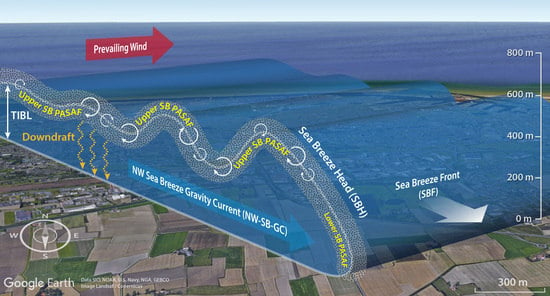
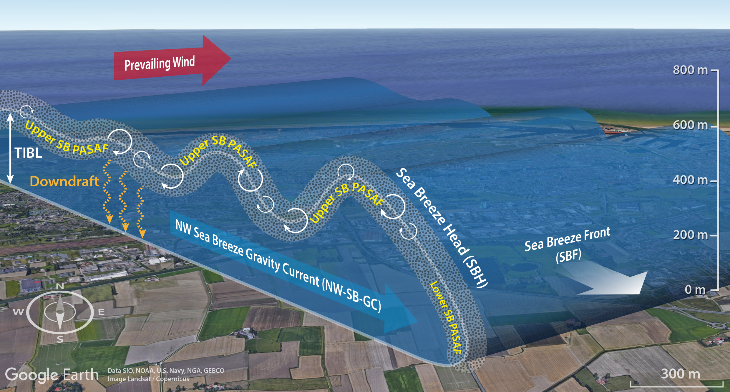
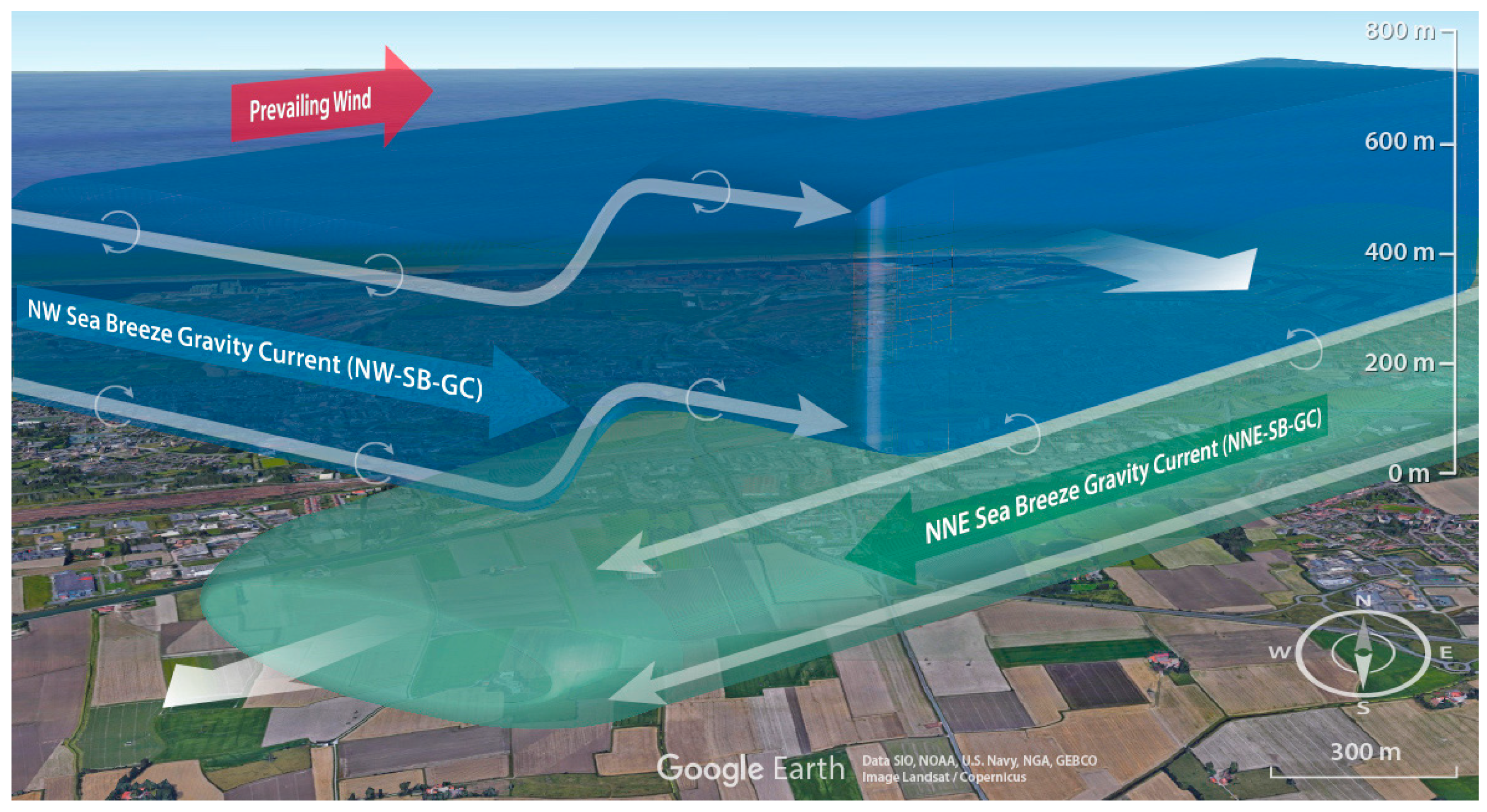
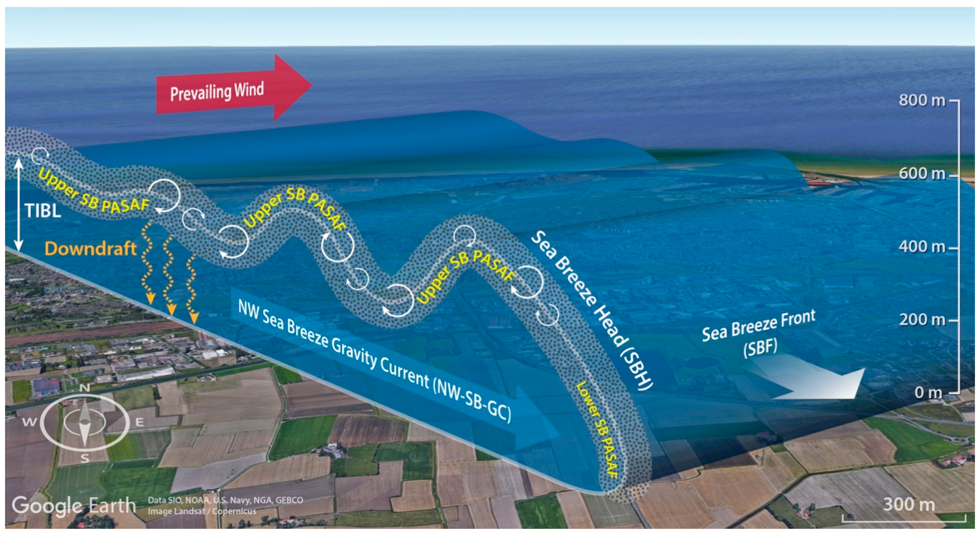
temporal and spatial evolution of the SB dynamical structure (ABL, SB system including the SB fronts, SB gravity currents),
-
evolution of the meteorological and aerosol (optical properties) vertical profiles, using in situ and remote sensing techniques, on a daily timescale, under the influence of SB,
-
SB potential effect to generate thermodynamically conditions favoring secondary aerosol formation,
-
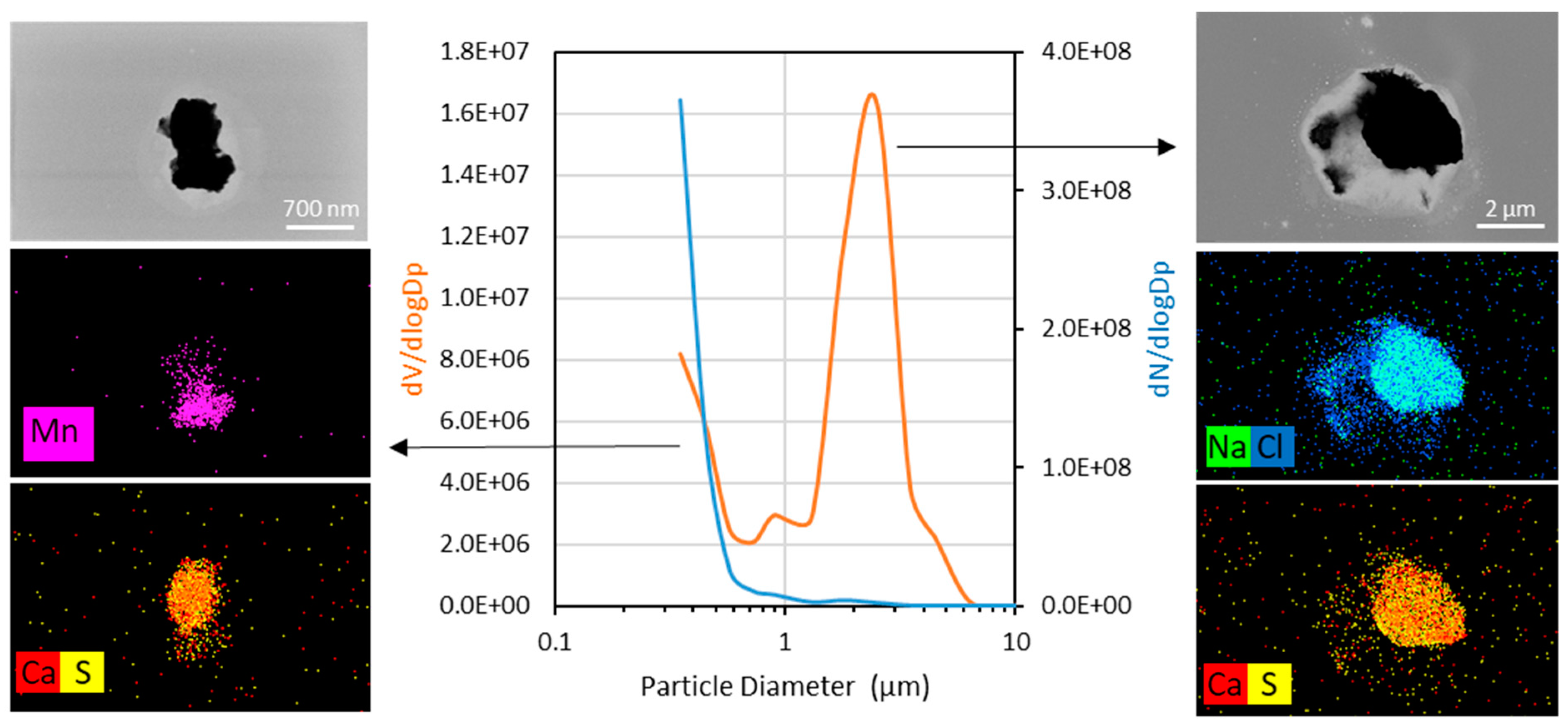
size distribution, morphology and chemical composition of aerosols collected during the SB period,
-
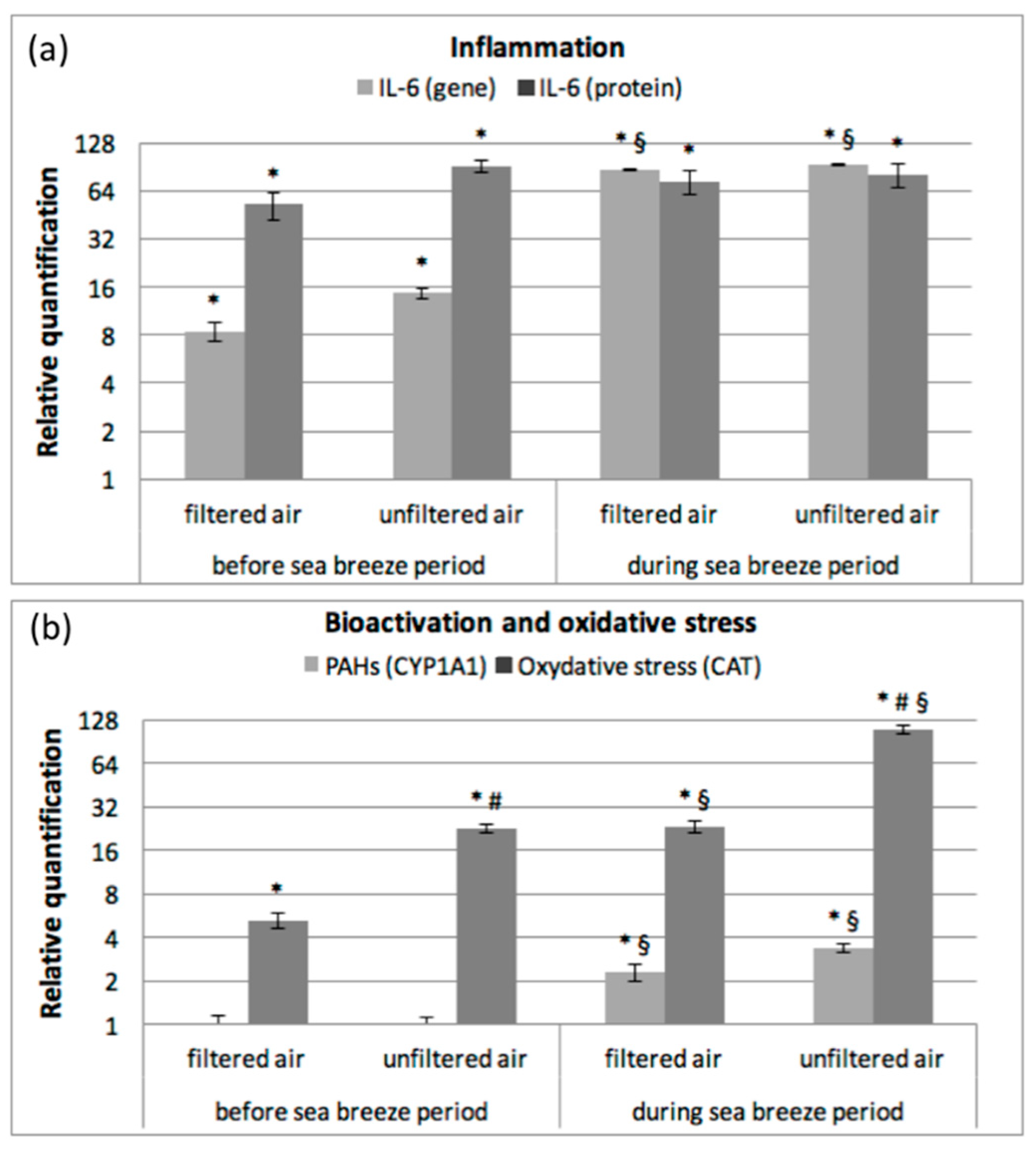
oxidative stress and inflammation processes in human lung cells exposed during SB.
This paper is organized as follows: in Section 2, the experimental setup and the methodology used to combine remote sensing and in situ instruments will be described; in Section 3, we will present the results of and discussions about the case study of an SB event; and Section 4 will conclude the paper.

2. Materials and Methods

We applied a systemic approach (Figure 1a) in which all the system components (aerosols, gases, ABL, SB, toxicology) were considered in synergy to thoroughly identify the specific emerging properties of each component and focus on the interactions between all system components. The investigation of all these processes requires measurements with high temporal resolution and large spatial flexibility. Remote sensing instruments and in situ instruments were then coupled during a two-month field campaign performed in summer 2017 in an industrialized and urbanized coastal environment in the North of France.

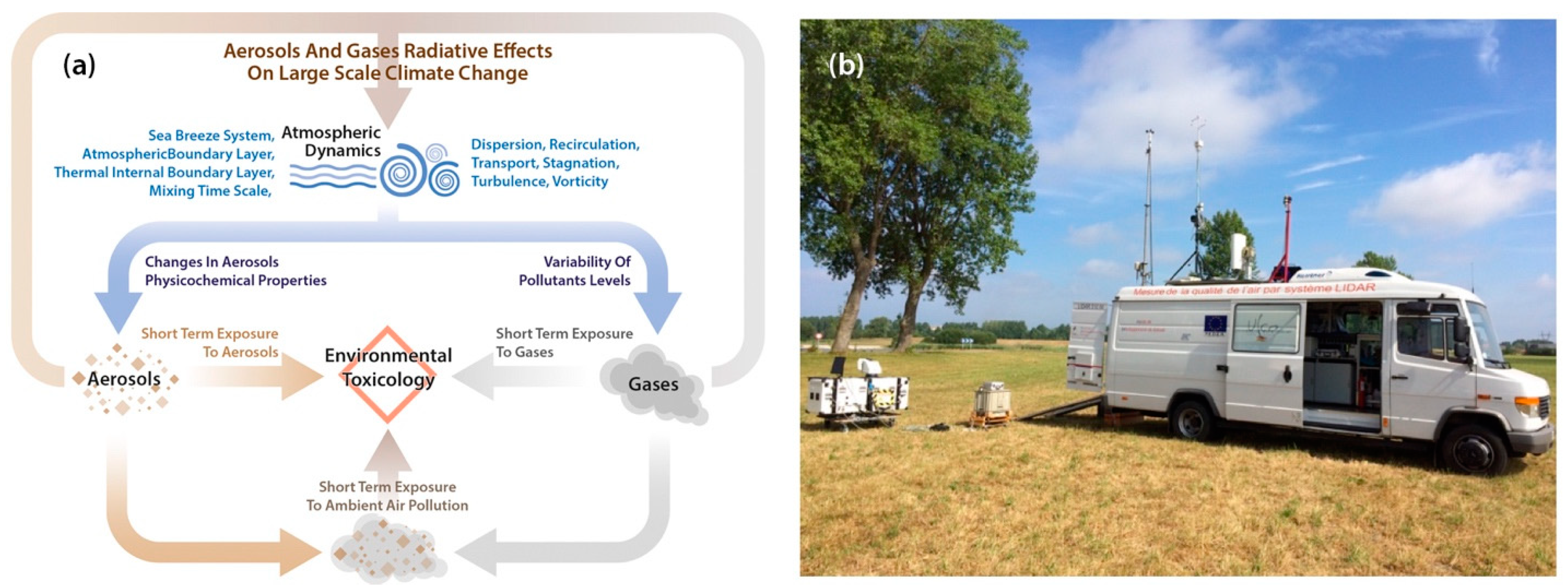
2.1. Atmospheric Mobile Unit (AMU)

In order to perform measurements with modern instrumentation combining remote sensing systems and in situ devices, the AMU, developed by the Université du Littoral Côte d’Opale (ULCO), gathered the main instruments as follow:
-
two scanning lidars (Doppler and elastic) and a meteorological station including a sonic anemometer,
-
a cascade impactor for aerosols sampling and chemical analyses, and two optical particle counters (OPCs),
-
and an in situ air-liquid interface (ALI) cells exposure device for the toxicity assessment.
During the field campaign in June and July 2017, the AMU was deployed in Dunkerque (Northern part of France) at about 5 km south of an industrialized area (50.99°N, 2.34°E) and 7 km south of the coastline oriented along the 75°–255° axis (Figure 2). The AMU was kept on alert throughout the campaign, monitoring the weather forecasts. As soon as the north winds were expected, the AMU was positioned south of the urban and industrial area, far enough from industrial emissions and emitted from stacks (up to 40 m high), to be able to capture pollutants at ground level. The daily precise position of the AMU was dictated by the local weather conditions.
The measurements were completed by continuous NOx and PM2.5 measurements at about 0.001 Hz (15 min) from the air quality monitoring network Atmo Hauts-de-France (ATMO HDF) located to the east of the study area (Figure 2).

2.2. Wind Measurements and Data Analysis Method

Wind fields were measured using a scanning wind lidar (Windcube WLS 100) manufactured by the LEOSPHERE company (www.leosphere.com). This pulsed Doppler lidar operates at 1543 nm with a repetition rate of 10 kHz and uses a heterodyne technique to measure the Doppler shift of laser radiation backscattered by aerosols [34,35].
A combination of range height indicator (RHI) and a Doppler beam swinging (DBS) techniques was used to determine the spatial structure and temporal evolution of the wind field and the vertical profile of the wind vector. The scanning programs consisted of 90° RHI toward the West, North West, North with 1° resolution and of a 75° elevation DBS in order to deduce wind vertical profiles.
A collocated ultrasonic anemometer operating at 10 Hz (model USA-1, Metek GmbH) providing 3D wind and temperature measurements was deployed on a 7 m mast.

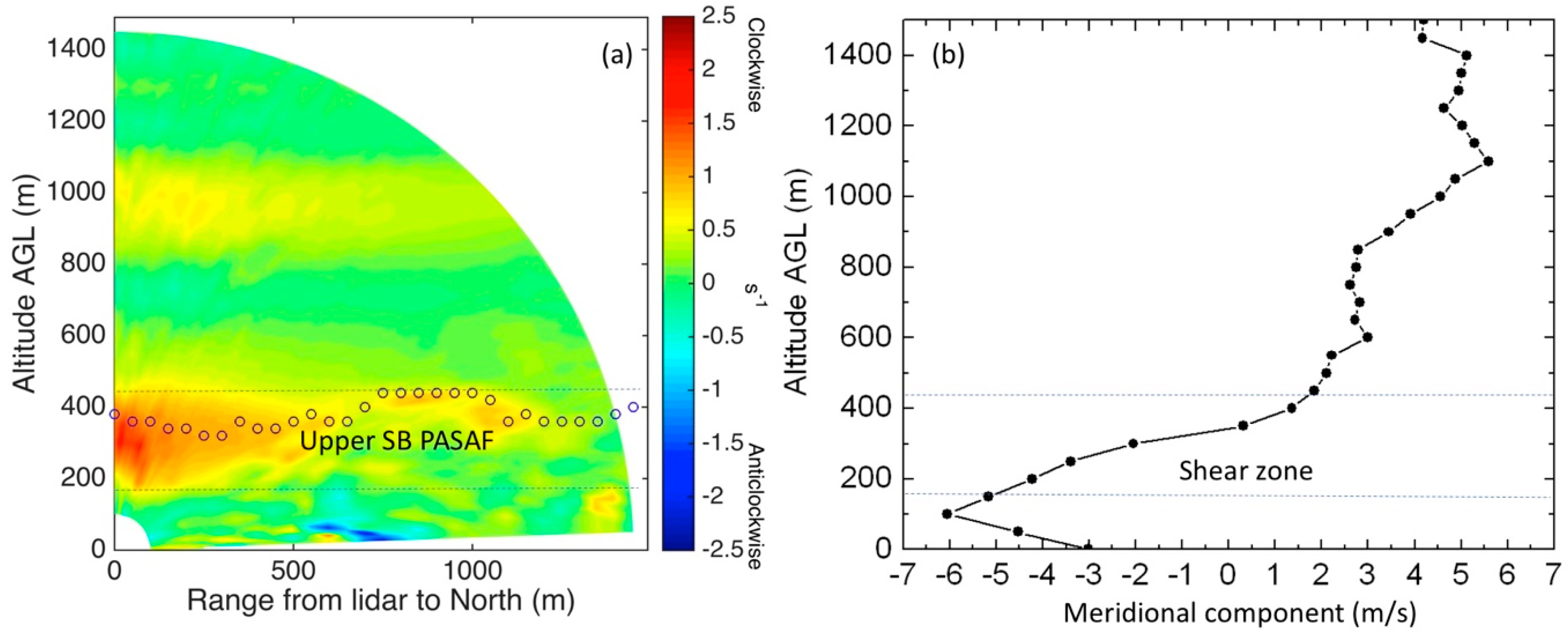
2.2.1. Two-Dimensional Flow Retrieval

The Doppler lidar measures the radial velocity component vr(r,θ,φ,t) at a range r, a time t, an elevation angle θ and an azimuthal angle φ. But vr contains the contributions from both the vertical w and horizontal wind vh components (eq.).
v r ( r , θ , φ , t ) = w ( r , θ , φ , t ) sin θ + v h ( r , θ , φ , t ) cos θ
Many studies have been devoted to extract both the vertical (w) and horizontal (vh) components by using simultaneous observations from two Doppler instruments [36,37,38,39]. Gao et al. [40] have proposed a new method based on a variational approach and the mass conservation equation to reduce the error accumulation in the estimation of the vertical velocity. In our study, we used Iwai et al.’s [41] method, which applies a modified two-dimensional variational method to a Doppler lidar RHI to retrieve the two-dimensional flow in vertical cross-sections. This method is more flexible in using Doppler data RHI in combination with other observations, such as DBS data, from only one Doppler device, as well as the use of various constraints to minimize a cost function.

2.2.2. SB Detection Structure

Different SB criteria were proposed to determine the SB events [42,43,44,45,46,47]. In our study, a set of strict criteria was selected to identify the SB onset time, during the field campaign period. These criteria are:
-
a simultaneously rapid change of the surface wind speed, the temperature, and the relative humidity measured from the AMU meteorological surface station during day time,
-
a shift in wind direction from offshore to onshore identified by the change of sign of the SB component (SBC) defined by KiranKumar et al. [47],
-
the presence of an SB front (SBF) and a gravity current (GC) coming from the sea.
In order to precisely deduce the structure of the SB system (SBF and GC top), we applied the transform covariance method on the slowness meridional component to each profile [22]. We also used the discrete Haar wavelet covariance transform method, which is well suited to identifying the transition zones. The transition zones correspond to the edges of the SB structure and are located in the vicinity of the SBF (when the SBF propagates against to the prevailing wind) and just below the shear zone corresponding to the SB GC top (where the flow direction changes from landward to seaward).

2.2.3. Characteristics of the Air Flows

The meteorological characteristics of the air flows observed over the site were deduced using the approach of Allwine and Whiteman [48]. The aim was to evaluate the specific atmospheric transport and diffusion conditions using three indicators: stagnation, recirculation, and ventilation. These indicators are not real measurements of the air mass transported (except under idealized homogeneous wind conditions), but give an idea of the transport and dispersion conditions of the air above the site by using a statistical approach. They are widely used to estimate flow meteorological characteristics over sites influenced by local effects such as SB or slope breeze in complex terrain [49,50,51,52]. In our study, we proposed to deduce the recirculation factor R by varying the transport period from 15 min to 5 h at the observation site from ultrasonic anemometer measurements (see Crumeyrolle et al. [22] for more details). The characteristics of the air flows within the surface layer, as well as the change in the turbulence quantities (turbulence kinetic energy dissipation rate, spectral scale) before and after the SBF penetration, were derived from the power spectrum of the wind velocity component by applying the inertial dissipation method to the ultrasonic anemometer measurements [53]. Moreover, to investigate the local mixing effect of SB, we estimated the vertical mean exchange velocity in mass Ve, corresponding to the local mean vertical turbulence flux of aerosol F normalized by the mean aerosol concentration (Section 2.4).

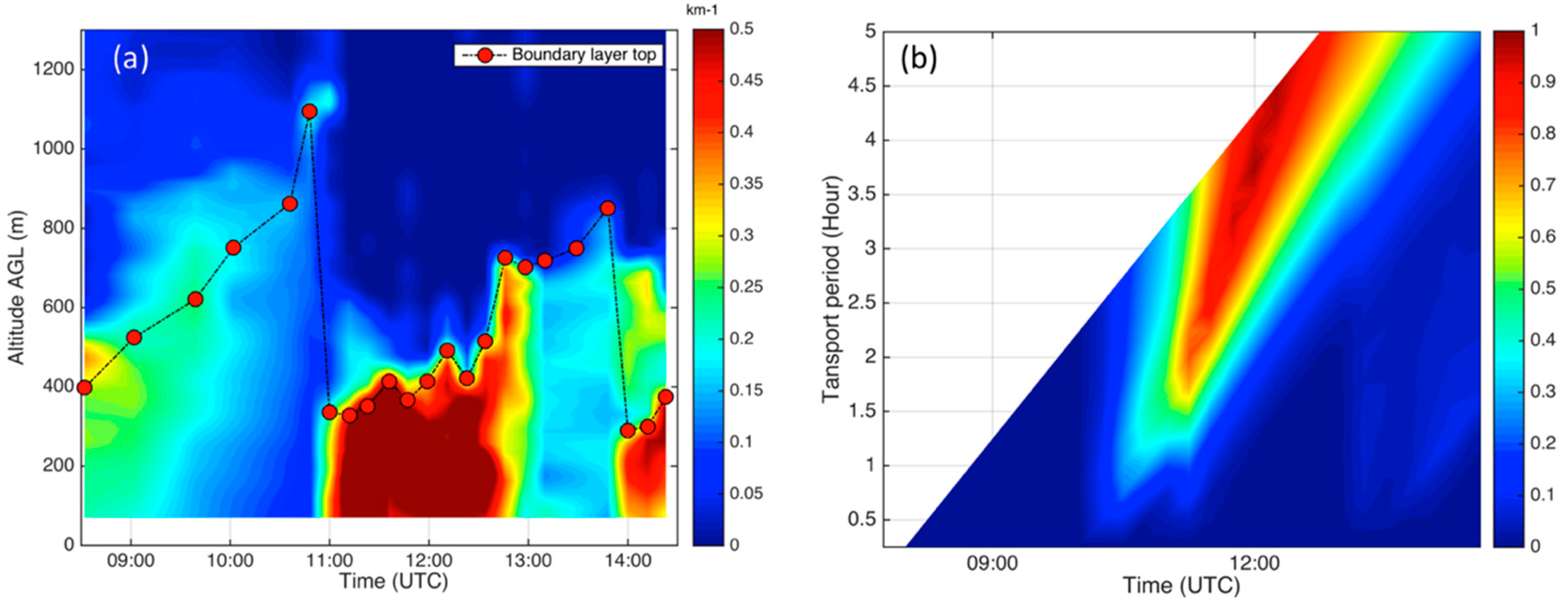
2.3. Lidar Inversion and ABL Top Detection Methodologies

A UV scanning lidar ALS 300, manufactured by the LEOSPHERE company, was used to deduced the ABL top along with the aerosols properties. This lidar operates with the third harmonic of a Nd-YAG laser at a wavelength of 355 nm. The energy pulse is about 16 mJ with a repetition rate of 20 Hz, and the spatial resolution is 15 m along each profile. The theoretical lidar blind distance r0 for optimal nearfield overlap is about 250 m. In order to reduce the blind distance from the lidar, a geometrical form factor (GFF) was deduced by using horizontal profile measurements in homogeneous clear atmosphere area before the start of the SB [54,55]. The experimentally-deduced GFF was applied to each profile obtained during the field campaign, thereby reducing the blind distance from 250 m to 105 m. This instrument was located on the roof of the AMU mounted on a telescopic mast. Continuous lidar monitoring was performed by vertical scans (RHI) from 2° to 90° elevation angle with 5° resolution along the NW azimuth angle, with 1000 shots per profile.

2.3.1. Lidar Inversion Methodology

The dispersion and transport of aerosols by coastal circulations are of interest for remote sensing applications. Due to sudden spatial and temporal changes of land/sea surface properties and due to uncertainties in the vertical distribution of aerosols, the retrieval of aerosol optical depth, extinction coefficient α, or backscatter coefficient β from lidar profiles is particularly difficult in coastal zones. Under several assumptions, the lidar signal can be inverted to determine aerosol optical properties. As an example, the lidar signal P can be inverted to determine the aerosol optical properties by using the well-known Klett Fernald method [56,57]. However, the lidar equation (2) is undetermined due to its dependence on the two-unknown β and α [58] at a range r.
P ( r ) = K β ( r ) / r 2 × e 2 r 0 r α ( r ) d r
where K is the constant of the lidar.
In the case of a single wavelength elastic backscatter lidar, the lidar ratio (LR; i.e., ratio of aerosol extinction-to-backscatter) can be estimated by using simultaneously the Aerosol Optical Depth (AOD) measurements, obtained by a sun photometer located in the close environment of our measurements site and integrated in the international Aerosol Robotic Network “Aeronet” (https://aeronet.gsfc.nasa.gov [59]). In order to increase the vertical resolution (altitude below 105 m and in the upper clear air of the free troposphere), we used all the profiles acquired for a zenith angle around 60° to invert the lidar signal.

2.3.2. ABL Top Dectection

In order to study the dynamics of the lower troposphere, the estimation of the ABL top is important, and it mainly relies on the detection of the vertical profiles of atmosphere variables (temperature, humidity and horizontal wind speed) or aerosol concentrations. Aerosol lidar is a powerful remote sensing instrument frequently used to retrieve ABL top through the detection of the vertical distribution of aerosol concentrations. Many different lidar techniques have been developed to detect ABL top which rely on the backscattered lidar signal [60], its first or second derivative [61,62], its variance [63], or fitting lidar signal techniques [64,65]. Methods based on the wavelet covariance transformation are robust, objective, semi-automated, efficient, and flexible methods, and they are less affected by signal noise than others [66,67,68,69,70]. In our study, we applied the wavelet covariance transform method by using the Haar wavelet mother. The wavelet covariance transform is defined as the convolution between the logarithm range-corrected lidar signal and the Haar wavelet. Locations of the local maxima of the wavelet covariance function are identified as the top of the ABL. In our case, the maximum of the wavelet variance, was used to deduce the dilation coefficient to determine the dominant atmospheric structure in the lidar signal which corresponds, in our case, to the ABL top [71].

2.4. Aerosols Sampling and Gas Measurements

Atmospheric particles were collected on Carbon Formvar© TEM grids adapted for individual-particle analysis. Sampling experiments were performed using a 3-stages cascade impactor (DekatiTM PM-10 type) installed at the top of a 3 m high mast, separating three size fractions according to particle aerodynamic diameters: 0.1–1.0 µm, 1.0–10 µm and >10µm. Individual particle analyses were performed by cryo-transmission scanning electron microscopy (cryo-TSEM), using a JEOLTM JSM7100F electron microscope, equipped with a cryogenic system QUORUMTM PP3010T and three BrukerTM X-ray energy dispersive spectrometers. The microscope operated at 15 kV with a current probe of 300 pA (working distance: 10 mm) and elemental maps were acquired at −100 °C for 5 min.
An optical particle counter (Grimm Aerosol Technik; model 1.108) was used to measure in situ particle size distribution in the 300 nm–20 µm (optical diameter) size range. A portable optical particle counter device, assembled in the laboratory, was also used for high measurement frequency. It was built around a commercial HK-A5 laser PM2.5/PM10 sensor, which counts all the particles with an optical diameter between 0.3 and 10 µm, with a frequency near 1 Hz. The comparison of both instruments was performed within the Chamber for Atmospheric Reactivity and Metrology of the Environment (CHARME) in 2017. The correlation factors as well as the normalized root mean square error (NRMSE) between PM1, PM2.5, and PM10 measured with the portable optical particle counter device and the GRIMM were found at 0.99 (NRMSE = 0.22), 0.98 (NRMSE = 0.13), 0.95 (NRMSE = 0.13). The inlet of the dust sensor was placed along the vertical mast near the ultrasonic anemometer. Additional analyzer measurements of gaseous air pollutants (nitric oxide, nitrogen dioxide) and mass concentrations of PM2.5 were provided by the instruments operated by the air quality monitoring network of ATMO HDF.
The particle vertical turbulence transport (particle fluxes) was calculated as the covariance between the fluctuations of the particle concentrations (measured with the portable optical particle counter) and the fluctuations of the vertical wind velocity (from the ultrasonic anemometer) using the eddy covariance (EC) method [72,73,74] with an averaging period of 30 min. The time delay (due to the length of the sampling inlets) was determined empirically, looking for the maximum cross-correlation absolute value between aerosol concentration and vertical wind velocity as a function of lag time. Due to the OPC low temporal resolution of concentration measurements, corrections for high frequency losses were needed to avoid an underestimation of particle turbulent fluxes using eddy-covariance method [75]. The correction ΔF of the flux F, used in this paper, is based on the convolution of co-spectral transfer function of the eddy covariance system H(f) and the co-spectrum S(f) given by:
Δ F F = 1 0 H ( f ) S ( f ) d f 0 S ( f ) d f
The co-spectral transfer function H(f), proposed by Horst [76] in the case of flux attenuation, depends mainly on atmospheric turbulence conditions (stability of the atmosphere, wind speed U, observation level z) and the time constant τ of the OPC. The time constant was determined by estimating, in the laboratory, that the time response to a concentration step was about 1.8 s [77], and atmospheric turbulence conditions were deduced from the sonic anemometer. The underestimation of particle turbulent fluxes has been deduced from the following analytical expression [76]:
Δ F F = 1 1 + ( 2 π n m τ U z ) α
with α = 7/8 for neutral and unstable stratification. The normal frequency nm corresponds to the maximum of frequency-weighted co-spectrum fS(f). The uncertainties due to the counting of discreet particles and the measurements of covariance were estimated, as described in Fairall et al. [78]. In order to limit the counting error, data from channels of the portable OPCs were pooled together. The average correction was about 21% which is comparable with the condensation particle counter (14%) and much larger than the one measured by the OPC (6%), used in Conte et al. [79]. Moreover, the Webb-Pearman-Leuning (WPL) correction have been applied to the particle turbulent fluxes measurements (with a Bowen ratio of 0.5), due to the effect of air density fluctuations corresponding to an average correction of about 5% [80]. The exchange velocity Ve was deduced by normalizing the particles fluxes with respect to the particle concentration [81]. Thus, positive values of Ve denote upwards transport whereas negative values of Ve describe downward transport.

2.5. Cells Air Exposure, Gene Expression and Inflammatory Determinations

In order to evaluate the toxicity of atmospheric aerosols occurring during SB events, we have developed an experimental device allowing, for the first time in a mobile unit, direct in vitro cell culture under real environmental conditions. Air was permanently pumped to the top of a 3 m high mast from outside of the AMU, before and during the SB periods. Cultured cells could then be exposed to the unfiltered or filtered pumped atmosphere. The purpose of filtration was to remove particles, in order to expose the cells only to the gas phase. Comparison of the response of cells after exposure to filtered and unfiltered air can be used to assess the toxicity attributable to particulate matter. The cellular model chosen was the BEAS 2B cell line (ATCC® CRL-9609), corresponding to human bronchial epithelial cells. BEAS 2B cells are frequently used in air liquid interface (ALI) exposure studies [82,83]. BEAS 2B cells were seeded on Transwell® inserts with LHC 9 medium in the culture room 24 h before the exposure. The cells were transported, just before the beginning of the exposure, from the laboratory to the AMU using an insulated cooler to minimize temperature variation. The medium was then removed from the apical side of the cells to expose them at the ALI. The exposure was performed using two Vitrocell® 6/3 CF Stainless exposure modules (Vitrocell GmbH, Germany). Each module was holding three Transwell® inserts, containing BEAS 2B cells, for the exposure over two hours to one of the two tested conditions: filtered air or unfiltered air. The air mixtures were delivered to the cells by a trumpet-shaped interface. To assess the toxicity of filtered and unfiltered air, unexposed cells cultured on Transwell® inserts from the same original cell population were kept in the cell incubator at 37 °C, and considered as a control. Five hours after the end of the exposure, supernatants and Transwell® inserts were collected and stored at −80 °C.
After total RNA extraction (Nucleospin® TriPrep kit, Macherey-Nagel), gene expression of interleukin-6 (IL-6), cytochrome P 450 1A1 (CYP1A1), and catalase (CAT) was measured by reverse transcription quantitative polymerase chain reaction (RT-qPCR) using a high capacity cDNA reverse transcription (RT) kit and Taqman® probe assays (Applied Biosystem, ThermoScientific) according to the manufacturer’s protocols. The ∆∆Ct method was applied after normalization by the 18S ribosomal RNA [84]. The results were expressed in the form of relative quantification (RQ) value. The latter represents the gene induction level in the air-exposed cells compared to the same gene induction level in the unexposed cells.
Concerning the inflammatory response of the exposed cells, the secretion of pro-inflammatory mediators by the exposed cells was assessed by quantifying the extracellular cytokine IL-6 using ELISA MAX™ kit (BioLegend, Ozyme) according to the manufacturer protocol.

3. Results and Discussion

During the EMMA field campaign, surface wind was mostly South Westerly (SW) but with moderate frequencies of North Northeasterly (NNE)—Northeasterly (NE) winds during June (about 20%) and of Northwesterly (NW)—North Northwesterly (NNW) winds during July (about 12%), corresponding to the influence of marine air mass in two different SB regimes (Figure 3).
Over these two months, 27 SB episodes were recorded coming from NW to NE, occurring mainly from the morning (about 9:00) up to the evening (about 20:00). However, among the 15 SB events observed during June 2017, 7 were related to NW surface winds, which tended to start later in the afternoon (15:00) and finish earlier (about 18:00) than NE SB cases. Although the occurrences of SB events were equivalent in July, 50% of SB events observed were a mixture of NE and NW SB regimes. The complexity of the dynamical circulation due to the interactions between NE and NW SB induced a high variability of aerosol physico-chemical properties and made it difficult to determine their toxicity. Therefore, in order to investigate the role of atmospheric dynamics on the evolution of the aerosol variability and their toxicity, we focused our investigation on a case study when both NE and NW regimes were observed on the 4th of July 2017.

3.1. Impacts of SB on the Lower Troposphere

On the 4th of July 2017, the persistence of high pressure conditions (1021 hPa) over the North of France coupled with summer diurnal heating generated land–sea thermal contrasts. These contrasts lead to the development of SB circulation along the coastal area. To evaluate the mechanism of pollutant transport, the SB structural characteristics were documented by the Doppler lidar and the weather station. Figure 4 shows the time-height cross-section of the horizontal wind direction and speed deduced from the combination of Doppler lidar and ultrasonic anemometer measurements. During the morning, the main prevailing wind direction was SW above 500 m, while a low southeasterly (SE) wind with speed < 3 m/s was observed below 400 m, which corresponds to the land breeze advecting continental air mass toward the sea.
At about 11:00, the SB phenomenon was well detected by the change of the wind direction from SW to NW below 100 m and associated with the increase in the wind speed. The SB GC top, symbolized by red circles in Figure 4, was well stationary at the beginning of the SB occurrence at a height of about 400 m. A singularity, with a maximum height of about 700 m, was observed between 13:00 and 14:00. Figure 5 shows the range height indicator (RHI) meridional/zonal component in colour. White arrows were superimposed in order to indicate the vector sum of vertical and meridional/zonal wind velocities. In Figure 5a–c, the SB was characterized by a Northerly inflow near the surface coming from the sea and the SB structure edge is represented by blue circles. In Figure 5a, blue circles correspond to the SBF inland penetration (landward edge) located at about 500 m from the Doppler lidar (at 10:50) and to the sea breeze head (SBH). The SBH was located just above and behind the SBF [1], reaching a height of about 300–500 m, and was characterized mainly by downdraft reaching −1.5 m/s. The meridional component inside the SB flow was about 4 m/s and the SBF propagation speed was about 2 m/s, as deduced from the intercorrelation between two consecutive horizontal lidar profiles of each 90° RHI toward NW. This SBF speed is in good agreement with the theoretical value of the propagation speed, as reported by Simpson and Britter [85].
During the SB occurrence, the SB component (SBC) changed from negative to positive (Figure 6a) because the wind veered clockwise from offshore SE to onshore NW (Figure 6b). A simultaneously rapid change in the surface wind speed, temperature, mixing ratio, and turbulence parameters was also observed (Figure 6c–h). At the passage of the SBF, the wind speed increased from 1 m/s up to 4 m/s accompanied by a drop in air temperature of 2 °C and an increase of the mixing ratio from approximately 8.4 to 9.4 g/kg The advection of cool and moist air over warm land surface, associated with SB during the daytime, may modify the vertical structure of the ABL.
Figure 7a shows the ABL top evolution superimposed on the time-height section of the aerosol extinction coefficient deduced from the aerosol lidar measurements. The growth rate of the ABL top (entrainment velocity), easily deduced by the aerosol lidar, was about 240 m/h from 08:30 to 11:00. The ABL top reached the maximum height for this day at about 1100 m just before the SBF passage, and then collapsed down to 300 m due to the development of the TIBL associated with the SB event. After the SBF passage, the TIBL top was located in the vicinity of the GC top located at about 400 m up to 12:30. These dynamics processes have been confirmed by our previous studies devoted on the impact of a sea breeze on the boundary-layer dynamics and the atmospheric stratification in a coastal area of the North Sea [21,32,33].
A singularity period was then observed, at about 12:30, characterized by temporal discontinuities of the SB GC top and the TIBL top from about 400 m up to 700 m (Figure 4 and Figure 7a). Unlike the SBF passage (at about 11:00), the TIBL developed suddenly, leading to mixing and dilution into a thicker layer (Figure 7a). Simultaneously to the TIBL development, the relative humidity decreased and the temperature increased, which strongly suggested that another air mass was incoming. Moreover, Doppler lidar measurements indicated a sharp change of the wind direction (from NW to NNE) in the lower part of the SB, below 100 m (Figure 4). This specific stratification was linked to the NNE wind direction of the lower air mass coming from the sea. Indeed, this new lower air mass propagated toward the land at the surface and was surmounted by the NW SB GC top up to 700 m at 13:00 (Figure 5d). This phenomenon generated a double flow structure (DFS; Figure 8).
Hence, the DFS corresponded to two adjacent flows with a slight wind direction change, as can be seen from the RHI of meridional and zonal component (Figure 5c,d). The structure was clearly visible by combining both RHI where the meridional RHI represented the whole DFS coming from North below the altitude of 700 m and up to the range of about 1000 m from the lidar. The top of the upper flow (NW SB GC) is indicated with blue circles in the meridional RHI (Figure 5c) and the lower flow top with blue circles in the zonal RHI (Figure 5d). During this singularity period, the DFS was made of the superposition of two SB corresponding to the NNE SB and the NW SB GC top as shown on the conceptual scheme in Figure 8. The NNE SB formed from a much lower relative humidity air mass, resulting in a decrease in mixing ratio observed between 12:30 and 13:30. This double flow structure was not clearly visible to the aerosol lidar in Figure 7, since the aerosol extinction coefficient was relatively homogeneous over the entire thickness of the TIBL between 13:00 and 14:00. This was probably due to the growth of TIBL, which efficiently mixed aerosols inside the whole layer. The lifetime of the DFS was short (less than an hour) due to the instability of the atmosphere implying that the DFS vanished after 14:00.

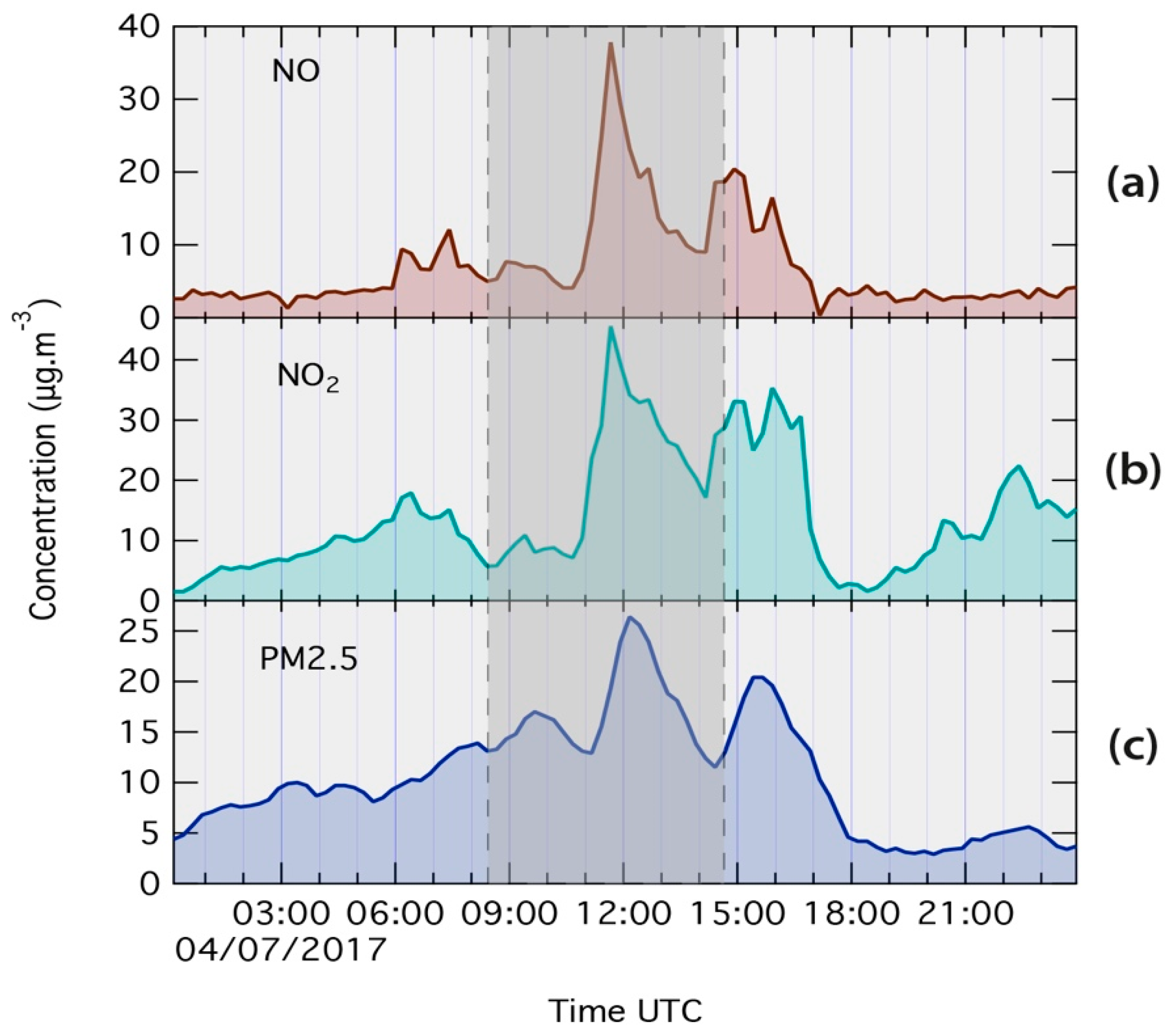
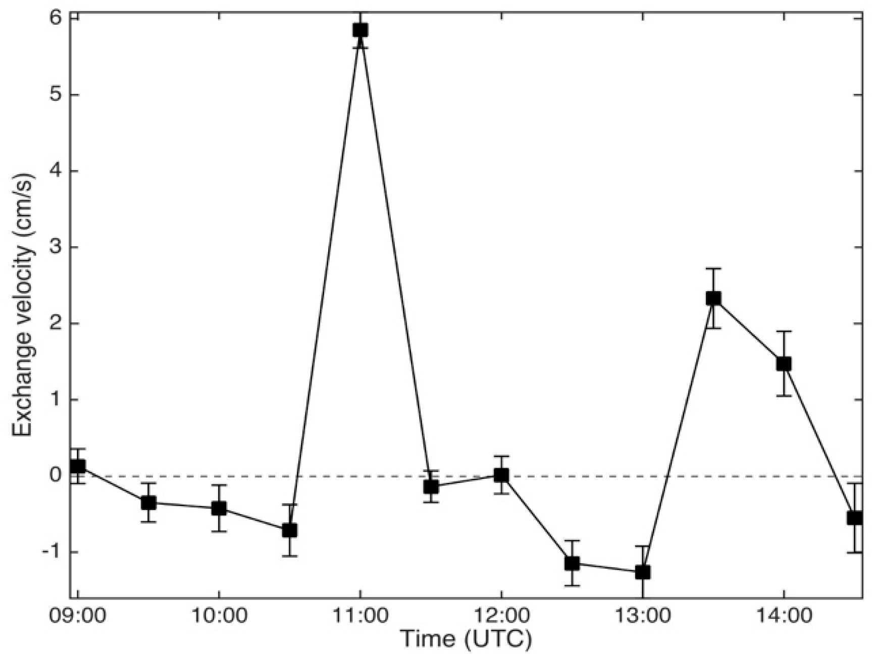
3.2. Impact of the SB on NOx and Aerosols

The SB occurrence was associated with high aerosol extinction coefficient values (>0.4 km−1) (Figure 7) and an increase of PM2.5 and NOx concentrations (Figure 9) just after the passage of the SB front, which can be explained by the development of the TIBL. Indeed, the ABL top decreased from about 1100 m down to 300 m, which limited the height of vertical mixing in the TIBL (Figure 7a).
Pollutants located in the TIBL can be trapped and mixed in this new layer, which was at a height 3.6 times lower than the one before the SBF passage. The mixing time scale τmix, corresponding to the time to mix pollutants from the top of the TIBL to ground level, can be estimated by using the energy dissipation rate ε [86] and the height of the TIBL top zi by:
τ m i x ( z i 2 ε ) 1 3
It was 619 s and 144 s before and after the SBF passage, respectively, so 4.3 times lower during the SB occurrence, indicating a strong mixing effect which may favor, for example, the rapid mixing of industrial plumes, emitted from chimneys, inside the TIBL by the well-known fumigation effects [21]. This SB crossed the industrial area, located in the NW of the studied site, and transported pollutants emitted in this polluted zone toward the land by the SB GC.
Moreover, high values of the recirculation factor R (>0.9) were obtained between 11:00 and 13:00, corresponding to a transport period of minimum 2.5–4.5 h (Figure 7b). This indicates that the air mass, observed at the sampling site between the SB occurrence and 13:00, was probably the same one as the one sampled from about 8:30 UTC until the SB arrival (11:00). However, this air mass was firstly enriched with urban and plume industrial emissions, during the initial transport between the studied site and the coast, and then diluted by dispersion during its transport in the SB GC. In addition to the recirculation conditions, low values of wind speed about one hour before the arrival of the SB front (Figure 6c) involved a tendency towards stagnation of the air. Pollutants freshly emitted from the industrialized area were slowly transported toward the sea by the land-breeze and stagnated until the SBF passage which spread underneath. Both layers were linked by the presence of downdrafts (Figure 5a) enriching the SB GC with freshly emitted pollutants. One can guess that the stagnation duration can be linked to the pollutant enrichment. Finally, all the pollutants mixed with cool and humid air enriched with marine particles were advected by the SB GC to the sampling site, leading to recirculation conditions. These results are consistent with our previous studies [21,23,32] focused on the investigation of the sea breezes impact on the pollution in urban and industrialized coastal area of the North Sea, by combining modeling and atmospheric dynamics measurements, in different time-scale (from few hours up to 6 months). Moreover, the one year study of pollutants’ spatial and temporal variations, based on hierarchical clustering analysis (HCA) applied in the urban area of Dunkerque, provided evidence of highest pollution episodes during sea breeze phenomenon, which is mainly responsible for the distribution and recirculation of air pollutants during summer [30].
The number-size distribution of particles during this first peak of PM2.5 concentrations (Figure 10) indicated a high proportion of fine particles (with diameter below 500 nm), while the volume-size distribution indicates a major mode of coarse particles centered on 2–3 µm. Individual particle analyses performed using cryo-TSEM-EDX on 536 particles highlighted a high fraction of submicronic particles contained a high fraction of secondary compounds such as nitrate (20.6% of analyzed particles) or oxidized organic compounds (66.9% of analyzed particles), which may result from nucleation and/or condensation of gaseous species after photo-oxidation. The formation of these particulate secondary compounds, by formation of new particles or by growth of pre-existing particles, was enhanced here by high concentrations of condensable gaze and vapors, and important solar luminosity. In these atmospheric conditions, a high proportion of atmospheric particles, notably micronic, are generally complex mixtures resulting from the aggregation of preexisting particles and from the condensation of volatile compounds on their surface [87,88]. The elemental maps, presented in Figure 10, illustrate these typical complex particles: on the left, a submicronic particle aggregating manganese oxide and gypsum (containing Ca and S); and on the right, an aqueous sea-salt particle (containing Na and Cl) including gypsum particles (containing Ca and S), poorly soluble in water. In conclusion, all of this information demonstrates that a high fraction of submicronic particles is a mixture of primary and secondary compounds resulting from condensation/aggregation processes during atmospheric transport, as already observed in the industrial and coastal urban environment [87,88]. The high turbulence in the SB gravity current and the high probability of air mass recirculation between 12:30 and 13:30 can explain the significant proportion of these complex mixtures.
Although, traffic and industrial emissions are major precursors for fine mode aerosols [89,90,91,92], secondary aerosol (SA) formation, due to photo-oxidation processes of marine precursors, may also contribute to the increase of PM2.5 concentration in coastal areas [91,92,93,94]. It can be notably explained in clean coastal environment by “new particle formation”, process for which photo-oxidized volatile species under relatively low PM concentrations, so low aerosol surface area leads to nucleation events [95,96,97,98]. This gas to particle conversion involves the initial formation of a critical cluster from super-saturated gaseous precursors [91,99,100,101]. The presence of significant turbulence in the boundary layer plays an important role in this cluster formation induced by microscale fluctuations in the humidity and temperature modifying super-saturation of gaseous precursors [102,103,104]. Otherwise, in coastal environments with higher PM2.5 concentrations, the large surface area of pre-existing particles can serve as a condensation sink for low volatile gaseous species, to the detriment of the nucleation and therefore of new particle formation [92], but also leading to an increase in PM2.5 concentrations. Moreover, high relative humidity conditions are favorable to the formation of secondary inorganic aerosols, such as sulphate formation by aqueous-phase oxidation of SO2 in aerosol water and heterogeneous reaction of SO2 on aerosols surfaces involving aerosol water [105,106]. Thus, all these SA formation processes are favored by atmospheric conditions encountered during this case study, such as temperature/humidity fluctuations, boundary layer circulation, relatively high concentration of various precursor species, the ABL top dynamics or the mixing of contrasting air masses during SB event and resulting in multi scale turbulence [107,108,109,110]. Finally, Easter and Peters [111], as well as Nilsson [112] and Crumeyrolle et al. [110], found that secondary aerosol (SA) formation is likely to start in elevated parts of the ABL rather than near ground level, particularly due to the effect of turbulence mixing across temperature and humidity gradient between the ABL top and the free troposphere. However, this SA formation is possible if there are sufficient amounts of precursor gases in the one of contrasted air masses [99].
Hence, in our case, these conditions can be encountered during SB episodes, especially over the land (far from the industrial area) when a polluted, wet, and cold air mass (NW SB), meets the less polluted, warm, and dry air mass advected by the prevailing wind (land breeze). Assuming that SA formation could be enhanced by either intermittent mixing of both air masses with initially different temperatures and relative humidity, or by fluctuations caused by turbulence, there are large areas that can potentially lead to particle formation near the SB flow edge. In our study, these areas, called the potential area of SA formation (PASAF) can be observed lower near the ground, especially during the SBF passage or slightly higher in altitude around the SB GC top (Figure 11).
In the lower part of the PASAF, the SBF corresponds to the landward edge of the SB GC and it is associated with high cross-shore temperature (about 2 °C) and mixing ratio contrasts of 1 g/kg (Figure 6d,e). In the vicinity of the SBF, turbulence fluctuation of thermodynamics parameters, such as temperature, was observed. Indeed, Figure 6g shows a sudden increase of the temperature structure parameter CT2 (from 0.11 to 0.26 K/m2/3) generated by the interaction between the two different thermodynamic air masses. This effect can create favorable thermodynamic conditions to start SA formation, especially when maximum thermodynamic parameter fluctuations are observed [104]. Moreover, the SBF separated the enriched mixed polluted marine air mass (during recirculation conditions and after crossed the industrial area), which may contain sufficient amounts of precursor gases, to the less polluted continental air, advected toward the sea by the prevailing wind (Figure 5, Figure 6b,c and Figure 9).
In the upper part of the PASAF and in the vicinity of the GC/TIBL top, the shear component reached values up to 0.03 s−1 after the SBF passage (Figure 4 and Figure 12). This shear zone was produced by the friction interaction between both layers (marine and continental) consisting of landward wet marine enriched polluted air mass and the relatively dry and less polluted seaward flow aloft (Figure 5b). According to Simpson et al. [113], Wakimoto et al. [114], and Chiba [115], Kelvin-Helmholtz billows (KHBs) may develop in the shear zone and may reinforce pollutants mixing between both layers due to turbulence effects generated in the vicinity of the SB GC top. Figure 12a shows the RHI vorticity deduced at about 20 min after the SBF passage. High vorticities were located in the vicinity of the SB GC top located at about 400 m (corresponding to the height of the TIBL top) and in the SB shear zone. At about 400 m, vorticity associated with the SB GC wave-like structure (Figure 12a), located at the interface between the SB GC top and the seaward flow aloft, may produce non-linear mixing between both adjacent layers within the 50 to 200 m layer, and may favor thermodynamic conditions for SA formation in the upper part of the SB GC structure. In this case, a part of the PM2.5 collected at ground level, can be explained by the vertical downward transport of freshly formed secondary aerosols from the upper PASAF (Figure 11).
To investigate this local mixing effect of the SB, the exchange velocity Ve at 30 min average was calculated and plotted in Figure 13. Ve temporal variability indicates the ability of turbulence motion to contribute to upward and downward transport of particles. During this study, two peaks were observed, corresponding to the SB passage and to the double flow structure (DFS) occurrence. The first peak, corresponding to high value of Ve (6 cm/s), was obtained during the SBF passage and highlights intense upward aerosol transport. Similar quick change in measured Ve (from negative to positive), observed during the SBF passage, has also been observed in the Venice area [116]. Indeed, the convergence zone generated by the meeting of two opposite air masses lead to an updraft at the SBF. Then, after the SB passage, the Ve was negative down to −1.3 cm/s, corresponding to downward aerosol transport until 13:00. The large downward flux confirms the hypothesis that secondary aerosols, freshly formed in the upper PASAF, could be transported at the surface by downdraft turbulence vertical transport.
During the DFS, observed between 12:30 and 14:00, one can note a significantly decrease of NOx and PM2.5 concentrations (Figure 9) highlighted by low aerosol extinction in the TIBL (<0.2 km−1, Figure 7). At 14:00, corresponding to the end of the DFS period, aerosol extinction increased sharply probably due to the drop of the TIBL from 800 down to 300 m. As the NNE SB GC did not cross the industrial area and the thickness of TIBL was relatively high; the pollutant concentrations were low (starting around 13:00, Figure 6 and Figure 8). At 14:00 (end of the DFS), the NNW SB GC reached one more time the ground at the measurement site associated with an increase of the pollutant concentrations trapped within a thin TIBL (thickness of 300 m).

3.3. Consequence of Short Term Exposure to Ambient Air Pollution During the SB Event

The control of pollutant levels by the SB dynamics can have a strong impact on air quality, particularly in coastal cities. Although long-term exposure to ambient air pollution is deemed to be a major risk affecting human health, short-term exposure to high pollution events, and especially during specific meteorological conditions such as SB for which atmospheric dynamics control pollutant levels, can also have a significant impact on human health. Both particles and gases are acutely toxic at significant exposure. The impact of particles on the respiratory system depends on their characteristics (particle size, morphology or chemical composition) dictating their ability to penetrate the lungs and their reactivity, whereas the toxicity of gaseous pollutants depends solely on their reactivity [117].
In our study, we brought an in vitro exposure device to the field to assess the toxicity of real air. This approach is challenging because of the difficulty of safely transporting biological samples to the field. Moreover, the field site must be located quite close to the culture laboratory. Finally, sufficient controls have to be done to obtain trustworthy results [118]. A very few recent studies investigated the impact of real air (ambient or indoor air) on cultured human lung cells [118,119,120]. Firstly, to assess the indoor air quality of a pool, an ALI exposure device quite similar to the one used in our study was directly placed at the pool side of the non-swimmer pool [120]. Cells exposed over 2 h to the air pumped above the water surface produced IL-6 and IL-8. Secondly, a lung cell experiment was deployed in the field to examine toxicity of complex mixtures of ambient air pollutants [118]. The purpose of this study was to be used as a basis for future research, helping to determine which pollutants or combination of pollutants are most important to overall toxicity. Therefore, studies such as ours or that of Zanini’s team were carried out in order to understand the mechanisms of action of real atmospheric pollutant [119]. Relationships between aerosols variability due to SB dynamics and its toxicological impact in short-term and at local scale is also currently poorly understood. In order to investigate the impact of the SB dynamics on toxic effects on human health, human lung cells were exposed to the real ambient air, before and the during SB period. The air liquid interface (ALI) system used allows the exposure of human lung cells to gases and aerosols (unfiltered) and only gases (filtered). Therefore, the aerosol toxicity can be assessed comparing filtered and unfiltered samples, while the toxicity of the air (gas + aerosol) can be estimated by comparing both sampling periods. After the 2 h short-term exposure, the cell response to real air exposure was assessed by measuring the gene expression of the main contributor of three major mechanisms of action of atmospheric pollutants: inflammation by IL-6, bioactivation of organic compounds by CYP1A1, and oxidative stress by CAT (Figure 14).
The first mechanism of action studied was the initiation of an inflammatory response (Figure 14a). The gene expression level and protein secretion of the inflammation mediator IL-6 were measured. For all the exposures, the gene and secretion of IL-6 significantly increased compared to the unexposed cells. This observation is consistent with the literature presented earlier on measuring the toxicity of exposure to real air [120].
For all of the exposures the protein levels were quite similar before and during the SB period. However, the gene induction was higher in the cells exposed to air (filtered or unfiltered) during the SB period, in comparison to cells exposed before the SB arrival. The particle contribution to the induction of the inflammatory response was limited. This is highlighted by a small increase of IL-6 gene expression in the cells exposed to the unfiltered air when compared to the filtered one.
Then, in order to understand the impact of atmospheric composition on the cell response, gene expression level of CYP1A1, known to be induced by the exposure to polycyclic aromatic hydrocarbons (PAH) and to polychlorinated dibenzo-p-dioxins [121], as well as CAT, an antioxidant enzyme, was assessed. CYP1A1 gene expression in the cells was significantly induced by the 2 h exposition to air during SB period (Figure 14b). Thus, these results suggest that the concentrations of PAHs and/or of dioxins were significantly higher in the SB gravity current than in the air mass sampled before the arrival of the SB front. Since there was a difference in the gene induction between the cells exposed with or without air filtration, it seemed that PAHs and/or dioxins were both in the gaseous and particulate phases [122]. Given the PAH sources over the area, one can assume that they are mostly industrial.
All of the exposures to unfiltered or filtered air induced the gene expression of CAT (Figure 13b). Therefore, atmospheric pollutants were able to induce oxidative stress in exposed lung cells. Cells were exposed to a complex mixture that includes nitrogen dioxide or ozone. The exposure to particles NO2 and O3 was shown to cause inflammation in human cells exposed to air pollution [123]. Recently, lung cell cultures, grown at the ALI, were directly exposed to ambient air in summer or winter. PM and NOX, more concentrated in winter than in summer, were correlated to the induction of pro-inflammatory genes [124], while another study showed that ozone can be more toxic than NO2 [125]. For all the exposures, the air filtration (aerosol removal) decreased significantly this gene induction. This result showed that the particulate matter has an important role in the induction of oxidative stress. This was shown not only with both in vitro studies [126] and in humans exposed to air pollution [127], but also in a cellular studies of the oxidative potential [128,129]. The latter studies have shown the contribution of combustion sources to the oxidative potential of aerosols, confirming the importance of industrial and traffic-related emissions, particularly in terms of carbonaceous species, transition metals, and PAHs [130]. These compounds were already quantified in PM and linked to in vitro toxicity in previous studies conducted in the Dunkerque metropolitan area [131,132]. In a previous work, we collected PM samples according to the wind direction and the season, and we were able to show variations in the mechanisms of toxic action depending on the sources. Cell exposure to the different PM samples resulted in variations in the gene induction of CYP1A1 and IL-6 [133,134]. Comparison of the results described in this study with the literature carried out in cell culture laboratories shows the relevance of using the ALI device outdoors for direct exposure to real atmosphere. This kind of device seems to be well suited to the study of other situations and to the transposition to other cases. Finally, short-term exposure to ambient air pollution during specific SB conditions involves an increase of the oxidative stress and inflammation processes in exposed human lung cells.

4. Conclusions

An atmospheric mobile unit (AMU) was implemented during a field campaign performed at a representative site of urbanized and industrialized coastal environment of the North Sea (Northern France), to study the impact of sea breeze (SB) dynamics on aerosol properties, and especially their toxicity. This unit combined aerosol samplers, two scanning lidars (Doppler and elastic), two aerosol particle sizers and an air-liquid interface (ALI, Vitrocell®) in vitro cell exposure device.
The SB dynamics and structure were analyzed, with the aim to characterize the SB front (SBF), SB head (SBH), the SB gravity current (SB GC) to: (i) evaluate their abilities to efficiently mix different aerosol types and condensable gases; (ii) possibly favor the formation of secondary aerosols (SA); and (iii) modify the toxicity of atmospheric particles and gases. The advection of cool and moist air (SB) over warm land surface lead to the modification of the vertical structure of the atmospheric boundary layer (ABL). The results showed that after the SBF passage, the ABL top collapsed, which limits the height of vertical mixing in the thermal internal boundary layer (TIBL). The SB occurrence was generally associated with high aerosol extinction coefficient values (>0.4 km−1) and an increase of PM2.5 and NOx concentrations. These increases could be explained by the evolution of the TIBL, which was much lower than the one before the SBF passage and by the recirculation conditions, involving SB air mass enrichment, due to urban and industrial plume transport toward the land. The particle number-size distribution indicated a high proportion of fine particles (below 500 nm), while the volume-size distribution showed a major mode of coarse particles, centered on 2–3 µm. Individual particle analyses performed by cryo-TSEM-EDX highlighted that submicronic particles contained a high fraction of secondary compounds, such as nitrate or oxidized organic compounds, which may result from nucleation and/or condensation of gaseous species after photo-oxidation on pre-existing particles. A high proportion of complex mixtures resulting, notably, from particle aggregation processes was also observed. The high turbulence produced during the SB occurrence and the high probability of air masses recirculation may explain the significant proportion of these complex mixtures.
Moreover, secondary aerosols (SA) formation might be enhanced by intermittent mixing of both turbulence and temperature/humidity gradients between the two contrasted air masses (marine and continental). These potential areas of SA formation (PASAFs) were observed near the ground and higher in altitude around the SB GC top (400 m) during the SBF passage. The SBF separated the enriched and mixed polluted marine air mass, which may contain sufficient amounts of precursor gases, to the less polluted continental air, advected toward the sea by the prevailing wind. The upper part of the PASAF, close to the vicinity of the GC/TIBL top, was characterized by high vorticity and wind shear. In this case, part of the PM2.5 collected at ground level could come from downward vertical turbulence transport of freshly formed secondary aerosols from the upper PASAF. This effect was confirmed by negative exchange velocities observed after the SBF passage.
In some instances, short singularity periods were observed during SB, corresponding to a double flow structure. This consisted of two adjacent SB currents that induced an important increase of the TIBL top leading to pollutants dispersion. These periods were associated with a substantial decrease in aerosol mass concentrations.
Finally, this study is one of the first to bring cell cultures into the field to evaluate the harmfulness of a real environmental compartment. Atmospheric toxicity in the presence or absence of SB was demonstrated in human bronchial cells exposed in the field using an ALI exposure system. Our study showed the sensitivity of the developed device to discriminate the mechanisms of toxic action activated when exposed to different atmospheres, i.e., before or during sea breezes, or in the presence or absence of aerosols. Thus, the initiation of an inflammatory response and the occurrence of oxidative stress could be shown in the case of short exposure to real air. This toxicity was measured as stronger during the SB. In addition, these methodologies enabled us for the first time to understand the toxicity of a real mixture of gaseous and particulate air pollutants, as well as to isolate the particulate fraction in order to assess its own toxicity. Since there is a difference in the cell response between exposed cells with and without air filtration, it appears that both gas and particulate phases contribute to the harmfulness of atmospheric air. These results constitute a first indication for public health officials to: (i) prioritize air pollutants; and (ii) control these pollutants, thus protecting the health of inhabitants living in these multi-influenced urban zones.
In this study, the AMU has proved to be a reliable device, useful to better understand the impact of dynamics on the temporal variability of pollutants and the associated toxic effects. The results of this study are significant and scalable to other urbanized and industrialized coastal sites where air pollution is a major issue.

Author Contributions

Conceptualization, P.A., S.B., K.D., P.F. and M.F.; methodology, P.A., S.B., K.D., P.F., M.F., S.G., Y.L. and C.M.; software, P.A., M.F. and A.S. (Anton Sokolov); validation, P.A., S.B., S.C., K.D., M.F., S.G., Y.L. and C.M.; formal analysis, P.A., S.B., S.C., K.D., M.F., S.G., Y.L., C.M., S.R., F.G.S. and A.S. (Alexei Sentchev); investigation, P.A., S.B., S.C., K.D., P.F., M.F., S.G., Y.L., C.M. and F.G.S.; data curation, P.A., S.B., K.D., P.F., M.F., S.G., Y.L. and C.M.; writing—original draft preparation, P.A., S.B., K.D., P.F., M.F., S.G., Y.L. and C.M.; writing—review and editing, P.A., S.B., S.C., K.D., E.D., P.F., M.F., S.G., B.H., Y.L., C.M., S.R., A.S. (Anton Sokolov) and A.S. (Alexei Sentchev); visualization, P.A., S.B., K.D., M.F., S.G., Y.L. and C.M.; supervision, P.A. and P.F.; project administration, P.A., S.B., K.D., P.F. and M.F.; funding acquisition, P.A., S.B., K.D., P.F. and M.F. All authors have read and agreed to the published version of the manuscript.

Funding

This research was funded by the Région « Hauts de France » and the Ministère de l’Enseignement Supérieur et de la Recherche (CPER IRenE and Climibio), by the European Fund for Regional Economic Development, by the Université du Littoral Côte d’Opale (BQR UMA), by the Labex CaPPA (Chemical and Physical Properties of the Atmosphere), which is funded by the French National Research Agency through the PIA (Programme d’Investissement d’Avenir) under contract “ANR-11-LABX-0005-01”.

Acknowledgments

The authors would like to thank Atmo Hauts-de-France for providing the air quality monitoring network data of the study and Dunkerque Grand Littoral/Communauté Urbaine de Dunkerque for the permission to operate the field campaign in Dunkerque. The authors graciously acknowledge the field efforts of our collaborators Fabrice Cazier, Dorothée Dewaele, Paul Genevray, Coralie Pusca (Centre Commun de Mesures), Fabien Marteel, Jérôme Parmentier, Arnaud Deswelle, Frederic Anceau, Xavier Notredaeme (Service Technique du CGU de Dunkerque) and Jason Debailleul (Ecole polytechnique de l’Université d’Orléans). The authors gratefully thank Benoit Escorne (Pôle EMLM) for the design and production of AMU mechanical devices, Jerôme Parmentier for the AMU power supply network design and installation, Julien Ratynski (LPCA) and Véronique Vanvincq (Pôle EMLM/UCEIV) our excellent secretaries/managers, Xavier Secordel and Romain Lepez (IRENE) for the administrative support, Philippe Reignault (Pôle EMLM) and Hervé Delbarre (LPCA) for the administrative project support. In the memory of Daniel Boucher and Pirouz Shirali.

Conflicts of Interest

The authors declare no conflict of interest. The funding sponsors had no role in the design of the study; in the collection, analyses, or interpretation of data; in the writing of the manuscript; or in the decision to publish the results.

References

  1. Miller, S.T.K. Sea breeze: Structure, forecasting, and impacts. Rev. Geophys. 2003, 41, 1011. [Google Scholar] [CrossRef] [Green Version]
  2. Heal, M.R.; Quincey, P. The relationship between black carbon concentration and black smoke: A more general approach. Atmos. Environ. 2012, 54, 538–544. [Google Scholar] [CrossRef] [Green Version]
  3. Ge, J.M.; Su, J.; Fu, Q.; Ackerman, T.P.; Huang, J.P. Dust aerosol forward scattering effects on ground-Based aerosol optical depth retrievals. J. Quant. Spectrosc. Radiat. Transf. 2011, 112, 310–319. [Google Scholar] [CrossRef]
  4. Wang, J.; Ge, C.; Yang, Z.; Hyer, E.J.; Reid, J.S.; Chew, B.-N.; Mahmud, M.; Zhang, Y.; Zhang, M. Mesoscale modeling of smoke transport over the Southeast Asian Maritime Continent: Interplay of sea breeze, trade wind, typhoon, and topography. Atmos. Res. 2013, 122, 486–503. [Google Scholar] [CrossRef]
  5. Melas, D.; Ziomas, I.; Klemm, O.; Zerefos, C.S. Anatomy of the sea-Breeze circulation in Athens area under weak large-Scale ambient winds. Atmos. Environ. 1998, 32, 2223–2237. [Google Scholar] [CrossRef]
  6. Mastrantonio, G.; Viola, A.P.; Argentini, S.; Fiocco, G.; Giannini, L.; Rossini, L.; Abbate, G.; Ocone, R.; Casonato, M. Observations of sea breeze events in Rome and the surrounding area by a network of Doppler sodars. Bound.-Layer Meteorol. 1994, 71, 67–80. [Google Scholar] [CrossRef]
  7. Verma, S.; Priyadharshini, B.; Pani, S.K.; Bharath Kumar, D.; Faruqi, A.R.; Bhanja, S.N.; Mandal, M. Aerosol extinction properties over coastal West Bengal Gangetic plain under inter-seasonal and sea breeze influenced transport processes. Atmos. Res. 2016, 167, 224–236. [Google Scholar] [CrossRef]
  8. Rosenfeld, D.; Woodley, W.L.; Lerner, A.; Kelman, G.; Lindsey, D.T. Satellite detection of severe convective storms by their retrieved vertical profiles of cloud particle effective radius and thermodynamic phase. J. Geophys. Res. Atmos. 2008, 113. [Google Scholar] [CrossRef] [Green Version]
  9. Lee, Y.-G.; Lee, H.-W.; Kim, M.-S.; Choi, C.Y.; Kim, J. Characteristics of particle formation events in the coastal region of Korea in 2005. Atmos. Environ. 2008, 42, 3729–3739. [Google Scholar] [CrossRef]
  10. Fernández-Camacho, R.; Rodríguez, S.; De La Rosa, J.; Sánchez De La Campa, A.M.; Viana, M.; Alastuey, A.; Querol, X. Ultrafine particle formation in the inland sea breeze airflow in Southwest Europe. Atmos. Chem. Phys. 2010, 10, 9615–9630. [Google Scholar] [CrossRef] [Green Version]
  11. Piazzola, J.; Sellegri, K.; Bourcier, L.; Mallet, M.; Tedeschi, G.; Missamou, T. Physicochemical characteristics of aerosols measured in the spring time in the Mediterranean coastal zone. Atmos. Environ. 2012, 54, 545–556. [Google Scholar] [CrossRef]
  12. Alonso-Blanco, E.; Gómez-Moreno, F.J.; Artíñano, B.; Iglesias-Samitier, S.; Juncal-Bello, V.; Piñeiro-Iglesias, M.; López-Mahía, P.; Pérez, N.; Brines, M.; Alastuey, A.; et al. Temporal and spatial variability of atmospheric particle number size distributions across Spain. Atmos. Environ. 2018, 190, 146–160. [Google Scholar] [CrossRef]
  13. Augustin, P.; Delbarre, H.; Lohou, F.; Campistron, B.; Puygrenier, V.; Cachier, H.; Lombardo, T. Investigation of local meteorological events and their relationship with ozone and aerosols during an ESCOMPTE photochemical episode. Ann. Geophys. 2006, 24, 2809–2822. [Google Scholar] [CrossRef] [Green Version]
  14. Haeffelin, M.; Angelini, F.; Morille, Y.; Martucci, G.; Frey, S.; Gobbi, G.P.; Lolli, S.; O’Dowd, C.D.; Sauvage, L.; Xueref-Rémy, I.; et al. Evaluation of Mixing-Height Retrievals from Automatic Profiling Lidars and Ceilometers in View of Future Integrated Networks in Europe. Bound.-Layer Meteorol. 2012, 143, 49–75. [Google Scholar] [CrossRef]
  15. Derimian, Y.; Marie Cho, I.; Rudich, Y.; Deboudt, K.; Dubovik, O.; Laskin, A.; Legrand, M.; Damiri, B.; Koren, I.; Unga, F.; et al. Effect of sea breeze circulation on aerosol mixing state and radiative properties in a desert setting. Atmos. Chem. Phys. 2017, 17, 11331–11353. [Google Scholar] [CrossRef] [Green Version]
  16. Rückerl, R.; Phipps, R.P.; Schneider, A.; Frampton, M.; Cyrys, J.; Oberdörster, G.; Wichmann, H.E.; Peters, A. Ultrafine particles and platelet activation in patients with coronary heart disease-Results from a prospective panel study. Part. Fibre Toxicol. 2007, 4. [Google Scholar] [CrossRef] [PubMed] [Green Version]
  17. Tobías, A.; Rivas, I.; Reche, C.; Alastuey, A.; Rodríguez, S.; Fernández-Camacho, R.; Sánchez de la Campa, A.M.; de la Rosa, J.; Sunyer, J.; Querol, X. Short-Term effects of ultrafine particles on daily mortality by primary vehicle exhaust versus secondary origin in three Spanish cities. Environ. Int. 2018, 111, 144–151. [Google Scholar] [CrossRef]
  18. Barnes, P.J. Chronic obstructive pulmonary disease. N. Engl. J. Med. 2000, 343, 269–280. [Google Scholar] [CrossRef] [Green Version]
  19. Bowler, R.P.; Barnes, P.J.; Crapo, J.D. The role of oxidative stress in chronic obstructive pulmonary disease. COPD J. Chronic Obstr. Pulm. Dis. 2004, 1, 255–277. [Google Scholar] [CrossRef]
  20. Hylkema, M.N.; Sterk, P.J.; de Boer, W.I.; Postma, D.S. Tobacco use in relation to COPD and asthma. Eur. Respir. J. 2007, 29, 438–445. [Google Scholar] [CrossRef] [Green Version]
  21. Talbot, C.; Augustin, P.; Leroy, C.; Willart, V.; Delbarre, H.; Khomenko, G. Impact of a sea breeze on the boundary-Layer dynamics and the atmospheric stratification in a coastal area of the North Sea. Bound.-Layer Meteorol. 2007, 125, 133–154. [Google Scholar] [CrossRef]
  22. Crumeyrolle, S.; Augustin, P.; Rivellini, L.-H.; Choël, M.; Riffault, V.; Deboudt, K.; Fourmentin, M.; Dieudonné, E.; Delbarre, H.; Derimian, Y.; et al. Aerosol variability induced by atmospheric dynamics in a coastal area of Senegal, North-Western Africa. Atmos. Environ. 2019, 203, 228–241. [Google Scholar] [CrossRef]
  23. Sokolov, A.; Dmitriev, E.; Maksimovich, E.; Delbarre, H.; Augustin, P.; Gengembre, C.; Fourmentin, M.; Locoge, N. Cluster Analysis of Atmospheric Dynamics and Pollution Transport in a Coastal Area. Bound.-Layer Meteorol. 2016, 161, 237–264. [Google Scholar] [CrossRef]
  24. Gohm, A.; Harnisch, F.; Vergeiner, J.; Obleitner, F.; Schnitzhofer, R.; Hansel, A.; Fix, A.; Neininger, B.; Emeis, S.; Schäfer, K. Air Pollution Transport in an Alpine Valley: Results From Airborne and Ground-Based Observations. Bound.-Layer Meteorol. 2009, 131, 441–463. [Google Scholar] [CrossRef] [Green Version]
  25. Mu, Q.; Liao, H. Simulation of the interannual variations of aerosols in China: Role of variations in meteorological parameters. Atmos. Chem. Phys. Discuss. 2014, 14, 11177–11219. [Google Scholar] [CrossRef]
  26. Geng, F.; Hua, J.; Mu, Z.; Peng, L.; Xu, X.; Chen, R.; Kan, H. Differentiating the associations of black carbon and fine particle with daily mortality in a Chinese city. Environ. Res. 2013, 120, 27–32. [Google Scholar] [CrossRef]
  27. Lin, W.; Huang, W.; Zhu, T.; Hu, M.; Brunekreef, B.; Zhang, Y.; Liu, X.; Cheng, H.; Gehring, U.; Li, C.; et al. Acute respiratory inflammation in children and black carbon in ambient air before and during the 2008 Beijing Olympics. Environ. Health Perspect. 2011, 119, 1507–1512. [Google Scholar] [CrossRef] [Green Version]
  28. Higashi, T. Reprint of: Effects of Asian dust on daily cough occurrence in patients with chronic cough: A panel study. Atmos. Environ. 2014, 97, 544–551. [Google Scholar] [CrossRef] [Green Version]
  29. Lepers, C.; Dergham, M.; Armand, L.; Billet, S.; Verdin, A.; Andre, V.; Pottier, D.; Courcot, D.; Shirali, P.; Sichel, F. Mutagenicity and clastogenicity of native airborne particulate matter samples collected under industrial, urban or rural influence. Toxicol. In Vitro 2014, 28, 866–874. [Google Scholar] [CrossRef]
  30. Rimetz-Planchon, J.; Perdrix, E.; Sobanska, S.; Brémard, C. PM10 air quality variations in an urbanized and industrialized harbor. Atmos. Environ. 2008, 42, 7274–7283. [Google Scholar] [CrossRef]
  31. Roukos, J.; Locoge, N.; Sacco, P.; Plaisance, H. Radial diffusive samplers for determination of 8-h concentration of BTEX, acetone, ethanol and ozone in ambient air during a sea breeze event. Atmos. Environ. 2011, 45, 755–763. [Google Scholar] [CrossRef]
  32. Salvador, N.; Reis, N.C., Jr.; Santos, J.M.; Albuquerque, T.T.A.; Loriato, A.G.; Delbarre, H.; Augustin, P.; Sokolov, A.; Moreira, D.M. Evaluation of weather research and forecasting model parameterizations under sea-Breeze conditions in a North Sea coastal environment. J. Meteorol. Res. 2016, 30, 998–1018. [Google Scholar] [CrossRef]
  33. Boyouk, N.; Léon, J.-F.; Delbarre, H.; Augustin, P.; Fourmentin, M. Impact of sea breeze on vertical structure of aerosol optical properties in Dunkerque, France. Atmos. Res. 2011, 101, 902–910. [Google Scholar] [CrossRef]
  34. Kumer, V.-M.; Reuder, J.; Dorninger, M.; Zauner, R.; Grubišić, V. Turbulent kinetic energy estimates from profiling wind LiDAR measurements and their potential for wind energy applications. Renew. Energy 2016, 99, 898–910. [Google Scholar] [CrossRef] [Green Version]
  35. Ruchith, R.D.; Ernest Raj, P. Features of nocturnal low level jet (NLLJ) observed over a tropical Indian station using high resolution Doppler wind lidar. J. Atmos. Sol.-Terr. Phys. 2015, 123, 113–123. [Google Scholar] [CrossRef]
  36. Drechsel, S.; Mayr, G.J.; Chong, M.; Chow, F.K. Volume scanning strategies for 3D wind retrieval from dual-doppler lidar measurements. J. Atmos. Ocean. Technol. 2010, 27, 1881–1892. [Google Scholar] [CrossRef]
  37. Shapiro, A.; Robinson, P.; Wurman, J.; Gao, J. Single-Doppler Velocity Retrieval with Rapid-Scan Radar Data. J. Atmos. Ocean. Technol. 2003, 20, 18. [Google Scholar] [CrossRef] [Green Version]
  38. Parsons, D.B.; Kropfli, R.A. Dynamics and fine structure of a microburst. J. Atmos. Sci. 1990, 47, 1674–1692. [Google Scholar] [CrossRef] [Green Version]
  39. Doviak, R.J.; Ray, P.S.; Strauch, R.G.; Miller, L.J. Error estimation in wind fields derived from dual-Doppler radar measurement. J. Appl. Meteorol. 1976, 15, 868–878. [Google Scholar] [CrossRef]
  40. Gao, J.; Xue, M.; Shapiro, A.; Droegemeier, K.K. A Variational Method for the Analysis of Three-Dimensional Wind Fields from Two Doppler Radars. Mon. Weather Rev. 1999, 127, 15. [Google Scholar] [CrossRef]
  41. Iwai, H.; Murayama, Y.; Ishii, S.; Mizutani, K.; Ohno, Y.; Hashiguchi, T. Strong Updraft at a Sea-Breeze Front and Associated Vertical Transport of Near-Surface Dense Aerosol Observed by Doppler Lidar and Ceilometer. Bound.-Layer Meteorol. 2011, 141, 117–142. [Google Scholar] [CrossRef]
  42. Gustavsson, T.; Lindqvist, S.; Borne, K.; Bogren, J. A study of sea and land breezes in an archipelago on the west coast of Sweden. Int. J. Climatol. 1995, 15, 785–800. [Google Scholar] [CrossRef]
  43. Borne, K.; Chen, D.; Nunez, M. A method for finding sea breeze days under stable synoptic conditions and its application to the Swedish west coast. Int. J. Climatol. 1998, 18, 901–914. [Google Scholar] [CrossRef]
  44. Furberg, M.; Steyn, D.G.; Baldi, M. The climatology of sea breezes on Sardinia. Int. J. Climatol. 2002, 22, 917–932. [Google Scholar] [CrossRef]
  45. Steyn, D.G.; Kallos, G. A study of the dynamics of hodograph rotation in the sea breezes of Attica, Greece. Bound.-Layer Meteorol. 1992, 58, 215–228. [Google Scholar] [CrossRef]
  46. Porson, A.N.F.; Steyn, D.G.; Schayes, G. Formulation of an index for sea breezes in opposing winds. J. Appl. Meteorol. Climatol. 2007, 46, 1257–1263. [Google Scholar] [CrossRef] [Green Version]
  47. KiranKumar, N.V.P.; Jagadeesh, K.; Niranjan, K.; Rajeev, K. Seasonal variations of sea breeze and its effect on the spectral behaviour of surface layer winds in the coastal zone near Visakhapatnam, India. J. Atmos. Sol.-Terr. Phys. 2019, 186, 1–7. [Google Scholar] [CrossRef]
  48. Allwine, K.J.; Whiteman, C.D. Single-Station integral measures of atmospheric stagnation, recirculation and ventilation. Atmos. Environ. 1994, 28, 713–721. [Google Scholar] [CrossRef]
  49. Al-Khadouri, A.; Al-Yahyai, S.; Charabi, Y. Contribution of atmospheric processes to the degradation of air quality: Case study (Sohar Industrial Area, Oman). Arab. J. Geosci. 2015, 8, 1623–1633. [Google Scholar] [CrossRef]
  50. Chithra, V.S.; Shiva Nagendra, S.M. Impact of outdoor meteorology on indoor PM10, PM2.5 and PM1 concentrations in a naturally ventilated classroom. Urban Clim. 2014, 10, 77–91. [Google Scholar] [CrossRef]
  51. Venegas, L.E.; Mazzeo, N.A. Atmospheric stagnation, recirculation and ventilation potential of several sites in Argentina. Atmos. Res. 1999, 52, 43–57. [Google Scholar] [CrossRef]
  52. Crescenti, G.H. Meteorological measurements during the Lower Rio Grande Valley environmental study. Environ. Int. 1997, 23, 629–642. [Google Scholar] [CrossRef]
  53. Champagne, F.H.; Friehe, C.A.; LaRue, J.C. Flux measurements, flux-Estimation techniques, and fine-scale turbulence measurements in the unstable surface layer over land. J. Atmos. Sci. 1977, 34, 515–530. [Google Scholar] [CrossRef] [Green Version]
  54. Sasano, Y.; Shimizu, H.; Takeuchi, N.; Okuda, M. Geometrical form factor in the laser radar equation: An experimental determination. Appl. Opt. 1979, 18, 3908–3910. [Google Scholar] [CrossRef] [PubMed]
  55. Halldórsson, T.; Langerholc, J. Geometrical form factors for the lidar function. Appl. Opt. 1978, 17, 240–244. [Google Scholar] [CrossRef] [PubMed]
  56. Klett, J.D. Stable analytical inversion solution for processing lidar returns. Appl. Opt. 1981, 20, 211–220. [Google Scholar] [CrossRef] [Green Version]
  57. Fernald, F.G. Analysis of atmospheric lidar observations: Some comments. Appl. Opt. 1984, 23, 652–653. [Google Scholar] [CrossRef]
  58. Ansmann, A.; Engelmann, R.; Althausen, D.; Wandinger, U.; Hu, M.; Zhang, Y.; He, Q. High aerosol load over the Pearl River Delta, China, observed with Raman lidar and Sun photometer. Geophys. Res. Lett. 2005, 32, 1–4. [Google Scholar] [CrossRef]
  59. Holben, B.N.; Tanré, D.; Smirnov, A.; Eck, T.F.; Slutsker, I.; Abuhassan, N.; Newcomb, W.W.; Schafer, J.S.; Chatenet, B.; Lavenu, F.; et al. An emerging ground-Based aerosol climatology: Aerosol optical depth from AERONET. J. Geophys. Res. Atmos. 2001, 106, 12067–12097. [Google Scholar] [CrossRef]
  60. Boers, R.; Eloranta, E.W. Lidar measurements of the atmospheric entrainment zone and the potential temperature jump across the top of the mixed layer. Bound.-Layer Meteorol. 1986, 34, 357–375. [Google Scholar] [CrossRef]
  61. Flamant, C.; Pelon, J.; Flamant, P.H.; Durand, P. Lidar determination of the entrainment zone thickness at the top of the unstable marine atmospheric boundary layer. Bound.-Layer Meteorol. 1997, 83, 247–284. [Google Scholar] [CrossRef]
  62. Menut, L.; Flamant, C.; Pelon, J.; Flamant, P.H. Urban boundary-layer height determination from lidar measurements over the paris area. Appl. Opt. 1999, 38, 945–954. [Google Scholar] [CrossRef] [PubMed]
  63. Hooper, W.P.; Eloranta, E.W. Lidar measurements of wind in the planetary boundary layer: The method, accuracy and results from joint measurements with radiosonde and kytoon. J. Clim. Appl. Meteorol. 1986, 25, 990–1001. [Google Scholar] [CrossRef] [Green Version]
  64. Steyn, D.G.; Baldi, M.; Hoff, R.M. The detection of mixed layer depth and entrainment zone thickness from lidar backscatter profiles. J. Atmos. Ocean. Technol. 1999, 16, 953–959. [Google Scholar] [CrossRef]
  65. Kovalev, V.A.; Wold, C.; Petkov, A.; Hao, W.M. Alternative method for determining the constant offset in lidar signal. Appl. Opt. 2009, 48, 2559. [Google Scholar] [CrossRef] [Green Version]
  66. Davis, K.J.; Gamage, N.; Hagelberg, C.R.; Kiemle, C.; Lenschow, D.H.; Sullivan, P.P. An Objective Method for Deriving Atmospheric Structure from Airborne Lidar Observations. J. Atmos. Ocean. Technol. 2000, 17, 14. [Google Scholar] [CrossRef] [Green Version]
  67. Cohn, S.A.; Angevine, W.M. Boundary layer height and entrainment zone thickness measured by lidars and wind-Profiling radars. J. Appl. Meteorol. 2000, 39, 1233–1247. [Google Scholar] [CrossRef]
  68. Gan, C.-M.; Wu, Y.; Madhavan, B.L.; Gross, B.; Moshary, F. Application of active optical sensors to probe the vertical structure of the urban boundary layer and assess anomalies in air quality model PM2.5 forecasts. Atmos. Environ. 2011, 45, 6613–6621. [Google Scholar] [CrossRef]
  69. Pal, S.; Behrendt, A.; Wulfmeyer, V. Elastic-Backscatter-Lidar-Based characterization of the convective boundary layer and investigation of related statistics. Ann. Geophys. 2010, 28, 825–847. [Google Scholar] [CrossRef] [Green Version]
  70. Mao, F.; Gong, W.; Song, S.; Zhu, Z. Determination of the boundary layer top from lidar backscatter profiles using a Haar wavelet method over Wuhan, China. Opt. Laser Technol. 2013, 49, 343–349. [Google Scholar] [CrossRef]
  71. Gamage, N.; Hagelberg, C. Detection and analysis of microfronts and associated coherent events using localized transforms. J. Atmos. Sci. 1993, 50, 750–756. [Google Scholar] [CrossRef] [Green Version]
  72. Businger, J.A. Evaluation of the accuracy with which dry deposition can be measured with current micrometeorological techniques. J. Clim. Appl. Meteorol. 1986, 25, 1100–1124. [Google Scholar] [CrossRef] [Green Version]
  73. Buzorius, G.; Rannik, U.; Mäkelä, J.M.; Vesala, T.; Kulmala, M. Vertical aerosol particle fluxes measured by eddy covariance technique using condensational particle counter. J. Aerosol Sci. 1998, 29, 157–171. [Google Scholar] [CrossRef]
  74. Nilsson, E.D.; Rannik, Ü.; Kulmala, M.; Buzorius, G.; O’Dowd, C.D. Effects of continental boundary layer evolution, convection, turbulence and entrainment, on aerosol formation. Tellus Ser. B Chem. Phys. Meteorol. 2001, 53, 441–461. [Google Scholar] [CrossRef]
  75. Moore, C.J. Frequency response corrections for eddy correlation systems. Bound.-Layer Meteorol. 1986, 37, 17–35. [Google Scholar] [CrossRef]
  76. Horst, T.W. A simple formula for attenuation of eddy fluxes measured with first-Order-Response scalar sensors. Bound.-Layer Meteorol. 1997, 82, 219–233. [Google Scholar] [CrossRef]
  77. Doebelin, E.O.; Manik, D.N. Measurement Systems: Application and Design; McGraw Hill Higher Education: New York, NY, USA, 1990; pp. 104–194. [Google Scholar]
  78. Fairall, C.W. Interpretation of eddy-Correlation measurements of particulate deposition and aerosol flux. Atmos. Environ. 1984, 18, 1329–1337. [Google Scholar] [CrossRef]
  79. Conte, M.; Donateo, A.; Contini, D. Characterisation of particle size distributions and corresponding size-Segregated turbulent fluxes simultaneously with CO2 exchange in an urban area. Sci. Total Environ. 2018, 622–623, 1067–1078. [Google Scholar] [CrossRef]
  80. Webb, E.K.; Pearman, G.I.; Leuning, R. Correction of flux measurements for density effects due to heat and water vapour transfer. Q. J. R. Meteorol. Soc. 1980, 106, 85–100. [Google Scholar] [CrossRef]
  81. Deventer, M.J.; von der Heyden, L.; Lamprecht, C.; Graus, M.; Karl, T.; Held, A. Aerosol particles during the Innsbruck Air Quality Study (INNAQS): Fluxes of nucleation to accumulation mode particles in relation to selective urban tracers. Atmos. Environ. 2018, 190, 376–388. [Google Scholar] [CrossRef]
  82. Hiemstra, P.S.; Grootaers, G.; van der Does, A.M.; Krul, C.A.M.; Kooter, I.M. Human lung epithelial cell cultures for analysis of inhaled toxicants: Lessons learned and future directions. Toxicol. In Vitro 2018, 47, 137–146. [Google Scholar] [CrossRef] [PubMed]
  83. Méausoone, C.; El Khawaja, R.; Tremolet, G.; Siffert, S.; Cousin, R.; Cazier, F.; Billet, S.; Courcot, D.; Landkocz, Y. In vitro toxicological evaluation of emissions from catalytic oxidation removal of industrial VOCs by air/liquid interface (ALI) exposure system in repeated mode. Toxicol. In Vitro 2019, 58, 110–117. [Google Scholar] [CrossRef] [PubMed]
  84. Livak, K.J.; Schmittgen, T.D. Analysis of relative gene expression data using real-Time quantitative PCR and the 2-ΔΔCT method. Methods 2001, 25, 402–408. [Google Scholar] [CrossRef] [PubMed]
  85. Simpson, J.E.; Britter, R.E. A laboratory model of an atmospheric mesofront. Q. J. R. Meteorol. Soc. 1980, 106, 485–500. [Google Scholar] [CrossRef]
  86. Wehner, B.; Siebert, H.; Ansmann, A.; Ditas, F.; Seifert, P.; Stratmann, F.; Wiedensohler, A.; Apituley, A.; Shaw, R.A.; Manninen, H.E.; et al. Observations of turbulence-Induced new particle formation in the residual layer. Atmos. Chem. Phys. 2010, 10, 4319–4330. [Google Scholar] [CrossRef] [Green Version]
  87. Marris, H.; Deboudt, K.; Augustin, P.; Flament, P.; Blond, F.; Fiani, E.; Fourmentin, M.; Delbarre, H. Fast changes in chemical composition and size distribution of fine particles during the near-field transport of industrial plumes. Sci. Total Environ. 2012, 427–428, 126–138. [Google Scholar] [CrossRef]
  88. Setyan, A.; Flament, P.; Locoge, N.; Deboudt, K.; Riffault, V.; Alleman, L.Y.; Schoemaecker, C.; Arndt, J.; Augustin, P.; Healy, R.M.; et al. Investigation on the near-field evolution of industrial plumes from metalworking activities. Sci. Total Environ. 2019, 668, 443–456. [Google Scholar] [CrossRef]
  89. O’Dowd, C.; Hoell, C.; Hill, M. Particle formation and fate in the coastal environment (PARFORCE): Initial results from a dedicated nucleation field experiment. J. Aerosol Sci. 1999, 30, S125–S126. [Google Scholar] [CrossRef]
  90. Kunz, G.J.; O’Dowd, C.D.; De Leeuw, G. Aerosol generation by waves breaking on small islands and rocks near the Mace Head research station. J. Aerosol Sci. 2000, 31, S656–S657. [Google Scholar] [CrossRef]
  91. O’Dowd, C.D. Coastal new particle formation: Environmental conditions and aerosol physicochemical characteristics during nucleation bursts. J. Geophys. Res. 2002, 107, 8107. [Google Scholar] [CrossRef] [Green Version]
  92. Rodríguez, S.; Cuevas, E.; González, Y.; Ramos, R.; Romero, P.M.; Pérez, N.; Querol, X.; Alastuey, A. Influence of sea breeze circulation and road traffic emissions on the relationship between particle number, black carbon, PM1, PM2.5 and PM2.5–10 concentrations in a coastal city. Atmos. Environ. 2008, 42, 6523–6534. [Google Scholar] [CrossRef]
  93. Kleefeld, C.; O’Reilly, S.; Jennings, S.G.; Becker, E.; O’Dowd, C.; Kunz, G.; De Leeuw, G. Aerosol scattering: Relation to primary and secondary aerosol production in the coastal atmosphere during the parforce campaign. J. Aerosol Sci. 2000, 31, S658–S659. [Google Scholar] [CrossRef]
  94. Ahlm, L.; Liu, S.; Day, D.A.; Russell, L.M.; Weber, R.; Gentner, D.R.; Goldstein, A.H.; Di Gangi, J.P.; Henry, S.B.; Keutsch, F.N.; et al. Formation and growth of ultrafine particles from secondary sources in Bakersfield, California. J. Geophys. Res. Atmos. 2012, 117. [Google Scholar] [CrossRef]
  95. Coe, H.; Williams, P.I.; McFiggans, G.; Gallagher, M.W.; Beswick, K.M.; Bower, K.N.; Choularton, T.W. Behavior of ultrafine particles in continental and marine air masses at a rural site in the United Kingdom. J. Geophys. Res. Atmos. 2000, 105, 26891–26905. [Google Scholar] [CrossRef] [Green Version]
  96. Martin, C.L.; Longley, I.D.; Dorsey, J.R.; Thomas, R.M.; Gallagher, M.W.; Nemitz, E. Ultrafine particle fluxes above four major European cities. Atmos. Environ. 2009, 43, 4714–4721. [Google Scholar] [CrossRef]
  97. Pirjola, L.; O’Dowd, C.D.; Brooks, I.M.; Kulmala, M. Can new particle formation occur in the clean marine boundary layer? J. Geophys. Res. Atmos. 2000, 105, 26531–26546. [Google Scholar] [CrossRef] [Green Version]
  98. De Leeuw, G.; Kunz, G.J.; Buzorius, G.; O’Dowd, C.D. Meteorological influences on coastal new particle formation. J. Geophys. Res. Atmos. 2002, 107. [Google Scholar] [CrossRef] [Green Version]
  99. Kulmala, M.; Vehkamäki, H.; Petäjä, T.; Dal Maso, M.; Lauri, A.; Kerminen, V.-M.; Birmili, W.; McMurry, P.H. Formation and growth rates of ultrafine atmospheric particles: A review of observations. J. Aerosol Sci. 2004, 35, 143–176. [Google Scholar] [CrossRef]
  100. Curtius, J. Nucleation of atmospheric aerosol particles. C. R. Phys. 2006, 7, 1027–1045. [Google Scholar] [CrossRef]
  101. Zhang, R. Getting to the critical nucleus of aerosol formation. Science 2010, 328, 1366–1367. [Google Scholar] [CrossRef] [Green Version]
  102. Bigg, E.K. A mechanism for the formation of new particles in the atmosphere. Atmos. Res. 1997, 43, 129–137. [Google Scholar] [CrossRef]
  103. Babu, S.S.; Kompalli, S.K.; Moorthy, K.K. Aerosol number size distributions over a coastal semi urban location: Seasonal changes and ultrafine particle bursts. Sci. Total Environ. 2016, 563–564, 351–365. [Google Scholar] [CrossRef] [PubMed]
  104. Platis, A.; Altstädter, B.; Wehner, B.; Wildmann, N.; Lampert, A.; Hermann, M.; Birmili, W.; Bange, J. An Observational Case Study on the Influence of Atmospheric Boundary-Layer Dynamics on New Particle Formation. Bound.-Layer Meteorol. 2016, 158, 67–92. [Google Scholar] [CrossRef]
  105. Han, B.; Wang, Y.; Zhang, R.; Yang, W.; Ma, Z.; Geng, W.; Bai, Z. Comparative statistical models for estimating potential roles of relative humidity and temperature on the concentrations of secondary inorganic aerosol: Statistical insights on air pollution episodes at Beijing during January 2013. Atmos. Environ. 2019, 212, 11–21. [Google Scholar] [CrossRef]
  106. Fang, Y.; Ye, C.; Wang, J.; Wu, Y.; Hu, M.; Lin, W.; Xu, F.; Zhu, T. Relative humidity and O3 concentration as two prerequisites for sulfate formation. Atmos. Chem. Phys. 2019, 19, 12295–12307. [Google Scholar] [CrossRef] [Green Version]
  107. Kulmala, M.; Toivonen, A.; Mäkelä, J.M.; Laaksonen, A. Analysis of the growth of nucleation mode particles observed in Boreal forest. Tellus Ser. B Chem. Phys. Meteorol. 1998, 50, 449–462. [Google Scholar] [CrossRef]
  108. Väkevä, M.; Hämeri, K.; Puhakka, T.; Nilsson, E.D.; Hohti, H.; Mäkelä, J.M. Effects of meteorological processes on aerosol particle size distribution in an urban background area. J. Geophys. Res. Atmos. 2000, 105, 9807–9821. [Google Scholar] [CrossRef] [Green Version]
  109. Russell, L.M.; Mensah, A.A.; Fischer, E.V.; Sive, B.C.; Varner, R.K.; Keene, W.C.; Stutz, J.; Pszenny, A.A.P. Nanoparticle growth following photochemical α- and β-Pinene oxidation at Appledore Island during International Consortium for Research on Transport and Transformation/Chemistry of Halogens at the Isles of Shoals 2004. J. Geophys. Res. Atmos. 2007, 112. [Google Scholar] [CrossRef]
  110. Crumeyrolle, S.; Manninen, H.E.; Sellegri, K.; Roberts, G.; Gomes, L.; Kulmala, M.; Weigel, R.; Laj, P.; Schwarzenboeck, A. New particle formation events measured on board the ATR-42 aircraft during the EUCAARI campaign. Atmos. Chem. Phys. 2010, 10, 6721–6735. [Google Scholar] [CrossRef] [Green Version]
  111. Easter, R.C.; Peters, L.K. Binary homogeneous nucleation: Temperature and relative humidity fluctuations, nonlinearity, and aspects of new particle production in the atmosphere. J. Appl. Meteorol. 1994, 33, 775–784. [Google Scholar] [CrossRef] [Green Version]
  112. Nilsson, E.D. The potential for atmospheric mixing processes to enhance the binary nucleation rate. J. Geophys. Res. Atmos. 1998, 103, 1381–1389. [Google Scholar] [CrossRef]
  113. Simpson, J.E. A comparison between laboratory and atmospheric density currents. Q. J. R. Meteorol. Soc. 1969, 95, 758–765. [Google Scholar] [CrossRef]
  114. Wakimoto, R.M.; Atkins, N.T. Observations of the sea-breeze front during CaPE. Part I: Single-Dopper, satellite, and cloud photogrammetry analysis. Mon. Weather Rev. 1994, 122, 1092–1114. [Google Scholar] [CrossRef] [Green Version]
  115. Chiba, O. The turbulent characteristics in the lowest part of the sea breeze front in the atmospheric surface layer. Bound.-Layer Meteorol. 1993, 65, 181–195. [Google Scholar] [CrossRef]
  116. Donateo, A.; Contini, D.; Belosi, F.; Gambaro, A.; Santachiara, G.; Cesari, D.; Prodi, F. Characterisation of PM2.5 concentrations and turbulent fluxes on a island of the Venice lagoon using high temporal resolution measurements. Meteorol. Z. 2012, 21, 385–398. [Google Scholar] [CrossRef] [Green Version]
  117. Buonanno, G.; Stabile, L.; Morawska, L. Personal exposure to ultrafine particles: The influence of time-activity patterns. Sci. Total Environ. 2014, 468–469, 903–907. [Google Scholar] [CrossRef] [Green Version]
  118. Vizuete, W.; Sexton, K.G.; Nguyen, H.; Smeester, L.; Aagaard, K.M.; Shope, C.; Lefer, B.; Flynn, J.H.; Alvarez, S.; Erickson, M.H.; et al. From the Field to the Laboratory: Air Pollutant-Induced Genomic Effects in Lung Cells. Environ. Health Insights 2015, 9. [Google Scholar] [CrossRef] [Green Version]
  119. Gualtieri, M.; Grollino, M.G.; Consales, C.; Costabile, F.; Manigrasso, M.; Avino, P.; Aufderheide, M.; Cordelli, E.; Di Liberto, L.; Petralia, E.; et al. Is it the time to study air pollution effects under environmental conditions? A case study to support the shift of in vitro toxicology from the bench to the field. Chemosphere 2018, 207, 552–564. [Google Scholar] [CrossRef]
  120. Schmalz, C.; Wunderlich, H.G.; Heinze, R.; Frimmel, F.H.; Zwiener, C.; Grummt, T. Application of an optimized system for the well-Defined exposure of human lung cells to trichloramine and indoor pool air. J. Water Health 2011, 9, 586–596. [Google Scholar] [CrossRef] [Green Version]
  121. Ma, Q. Induction of CYP1A1. The AhR/DRE paradigm: Transcription, receptor regulation, and expanding biological roles. Curr. Drug Metab. 2001, 2, 149–164. [Google Scholar] [CrossRef]
  122. Mandalakis, M.; Tsapakis, M.; Tsoga, A.; Stephanou, E.G. Gas-Particle concentrations and distribution of aliphatic hydrocarbons, PAHs, PCBs and PCDD/Fs in the atmosphere of Athens (Greece). Atmos. Environ. 2002, 36, 4023–4035. [Google Scholar] [CrossRef]
  123. Dauchet, L.; Hulo, S.; Cherot-Kornobis, N.; Matran, R.; Amouyel, P.; Edmé, J.-L.; Giovannelli, J. Short-term exposure to air pollution: Associations with lung function and inflammatory markers in non-Smoking, healthy adults. Environ. Int. 2018, 121, 610–619. [Google Scholar] [CrossRef] [PubMed]
  124. Bisig, C.; Petri-Fink, A.; Rothen-Rutishauser, B. A realistic in vitro exposure revealed seasonal differences in (pro-)inflammatory effects from ambient air in Fribourg, Switzerland. Inhal. Toxicol. 2018, 30, 40–48. [Google Scholar] [CrossRef] [PubMed]
  125. Mirowsky, J.E.; Dailey, L.A.; Devlin, R.B. Differential expression of pro-Inflammatory and oxidative stress mediators induced by nitrogen dioxide and ozone in primary human bronchial epithelial cells. Inhal. Toxicol. 2016, 28, 374–382. [Google Scholar] [CrossRef] [Green Version]
  126. Dergham, M.; Lepers, C.; Verdin, A.; Billet, S.; Cazier, F.; Courcot, D.; Shirali, P.; Garçon, G. Prooxidant and Proinflammatory Potency of Air Pollution Particulate Matter (PM2.5–0.3) Produced in Rural, Urban, or Industrial Surroundings in Human Bronchial Epithelial Cells (BEAS-2B). Chem. Res. Toxicol. 2012, 25, 904–919. [Google Scholar] [CrossRef]
  127. Wenten, M.; Gauderman, W.J.; Berhane, K.; Lin, P.-C.; Peters, J.; Gilliland, F.D. Functional variants in the catalase and myeloperoxidase genes, ambient air pollution, and respiratory-Related school absences: An example of epistasis in gene-environment interactions. Am. J. Epidemiol. 2009, 170, 1494–1501. [Google Scholar] [CrossRef] [Green Version]
  128. Janssen, N.A.H.; Yang, A.; Strak, M.; Steenhof, M.; Hellack, B.; Gerlofs-Nijland, M.E.; Kuhlbusch, T.; Kelly, F.; Harrison, R.; Brunekreef, B.; et al. Oxidative potential of particulate matter collected at sites with different source characteristics. Sci. Total Environ. 2014, 472, 572–581. [Google Scholar] [CrossRef] [Green Version]
  129. Chirizzi, D.; Cesari, D.; Guascito, M.R.; Dinoi, A.; Giotta, L.; Donateo, A.; Contini, D. Influence of Saharan dust outbreaks and carbon content on oxidative potential of water-Soluble fractions of PM2.5 and PM10. Atmos. Environ. 2017, 163, 1–8. [Google Scholar] [CrossRef]
  130. Harrison, R.M.; Yin, J. Particulate matter in the atmosphere: Which particle properties are important for its effects on health? Sci. Total Environ. 2000, 249, 85–101. [Google Scholar] [CrossRef]
  131. Billet, S.; Landkocz, Y.; Martin, P.J.; Verdin, A.; Ledoux, F.; Lepers, C.; André, V.; Cazier, F.; Sichel, F.; Shirali, P.; et al. Chemical characterization of fine and ultrafine PM, direct and indirect genotoxicity of PM and their organic extracts on pulmonary cells. J. Environ. Sci. 2018, 71, 168–178. [Google Scholar] [CrossRef]
  132. Billet, S.; Garçon, G.; Dagher, Z.; Verdin, A.; Ledoux, F.; Cazier, F.; Courcot, D.; Aboukais, A.; Shirali, P. Ambient particulate matter (PM2.5): Physicochemical characterization and metabolic activation of the organic fraction in human lung epithelial cells (A549). Environ. Res. 2007, 105, 212–223. [Google Scholar] [CrossRef] [PubMed]
  133. Dergham, M.; Lepers, C.; Verdin, A.; Cazier, F.; Billet, S.; Courcot, D.; Shirali, P.; Garçon, G. Temporal–spatial variations of the physicochemical characteristics of air pollution Particulate Matter (PM2.5–0.3) and toxicological effects in human bronchial epithelial cells (BEAS-2B). Environ. Res. 2015, 137, 256–267. [Google Scholar] [CrossRef] [PubMed]
  134. Lepers, C.; André, V.; Dergham, M.; Billet, S.; Verdin, A.; Garçon, G.; Dewaele, D.; Cazier, F.; Sichel, F.; Shirali, P. Xenobiotic metabolism induction and bulky DNA adducts generated by particulate matter pollution in BEAS-2B cell line: Geographical and seasonal influence. J. Appl. Toxicol. 2014, 34, 703–713. [Google Scholar] [CrossRef] [PubMed]
Figure 1. (a) Systemic scheme illustrating interactions between components of the studied system, (b) the atmospheric mobile unit (AMU) deployed during the Etude Mobile Multi-echelle Atmospherique (EMMA) campaign.
Remotesensing 12 00648 g001
Figure 2. (left) Map of North West Europe with the location of the study area (right) Experimental area on the 4th of July 2017. The yellow filled zone represents the industrialized area.
Remotesensing 12 00648 g002
Figure 3. Wind-rose diagrams observed at Dunkerque during (a) June 2017 and (b) July 2017.
Remotesensing 12 00648 g003
Figure 4. Time-height cross-section of the horizontal wind direction (arrows) and speed (color scale) at Dunkerque (Leftward and downward arrows represent, respectively, easterly wind and northerly wind). Red circles symbolized the sea breeze (SB) gravity current (GC) top.
Remotesensing 12 00648 g004
Figure 5. Range height indicator (RHI) of meridional component (colour), vector sum of vertical and meridional wind velocities (white arrows), edge of the SB structure (circles) (a) SB front at 10:50, (b) Northwesterly (NW) SB gravity current top at 11:20, (c) SB double structure top at 13:02, (d) RHI of zonal component (colour), vector sum of vertical and zonal wind velocities (white arrows), North Northeasterly (NNE) SB gravity current top (circles) at 12:58.
Remotesensing 12 00648 g005
Figure 6. Time series of (a) SB component (SBC), (b) wind direction (direction), (c) wind speed (Speed), (d) temperature (T), (e) mixing ratio (MR), (f) turbulence kinetic energy (TKE), (g) temperature structure parameter (CT2), (h) turbulence energy dissipation rate (ε).
Remotesensing 12 00648 g006
Figure 7. (a) Time-height cross-section of the aerosol extinction coefficient and atmospheric boundary layer (ABL) top symbolized by red circles deduced from the aerosol lidar, (b) Recirculation factor estimated from the sonic anemometer during the 4th of July.
Remotesensing 12 00648 g007
Figure 8. Conceptual scheme of the SB structure, illustrating the double flow structure observed during the singularity period, corresponding to the superposition of two SB.
Remotesensing 12 00648 g008
Figure 9. Time series of (a) NO, (b) NO2, (c) PM2.5 (Source: Atmo Hauts-de-France), grayed zone corresponds to the intensive observation period presented in Figure 6.
Remotesensing 12 00648 g009
Figure 10. Mean volume-size and number-size distribution of atmospheric aerosols collected on 4th of July 2017 from 12:20 to 13:30 UTC and elemental maps obtained by cryo-transmission scanning electron microscopy (cryo-TSEM)-EDX from a typical aggregate collected during this SB period.
Remotesensing 12 00648 g010
Figure 11. Conceptual scheme of the SB structure illustrating atmospheric conditions which may favor potential area of secondary aerosol formation (PASAF) process in the vicinity of the SB edge caused by the mixing of contrasting air masses (SB landward and seaward air masses) and turbulence effects.
Remotesensing 12 00648 g011
Figure 12. (a) RHI of meridional vorticity component between 11:19:24–11:20:53, blue circles symbolized the SB GC top estimated by the Haar wavelet covariance transform method, (b) vertical profile of meridional component at 11:19.
Remotesensing 12 00648 g012
Figure 13. Time evolution of the exchange velocity during the 4th of July 2017.
Remotesensing 12 00648 g013
Figure 14. Relative (in comparison with the unexposed cells) gene expression level and protein secretion of IL-6 (a) and expression level of xenobiotic metabolizing enzyme cytochrome P-450 1A1 (CYP1A1) and catalase (CAT) enzyme (b) of BEAS-2B cells exposed to filtered and unfiltered air using an Air-Liquid Interface system before and during the SB period. (*: significant induction compared to incubator control; #: significant induction between filtered air and unfiltered air; §: significant induction between before and during the SB period; p < 0.05).
Remotesensing 12 00648 g014

