Article

Monsoon Season Quantitative Assessment of Biomass Burning Clear-Sky Aerosol Radiative Effect at Surface by Ground-Based Lidar Observations in Pulau Pinang, Malaysia in 2014

1
CNR-IMAA, Contrada S. Loja, 85050 Tito Scalo (PZ), Italy
2
SSAI-NASA GSFC Code 612, Greenbelt Road Greenbelt, MD 20771, USA
3
School of Physics, Universiti Sains Malaysia, 11800 Penang, Malaysia
*
Author to whom correspondence should be addressed.
Remote Sens. 2019, 11(22), 2660; https://doi.org/10.3390/rs11222660
Submission received: 16 September 2019 / Revised: 5 November 2019 / Accepted: 8 November 2019 / Published: 14 November 2019
(This article belongs to the Special Issue Lidar Remote Sensing of Aerosols Observation)

Abstract

:
Direct and indirect aerosol effects are still one of the largest uncertainties related to the Earth energy budget, especially in a wild and remote region like South-East Asia, where ground-based measurements are still difficult and scarce, while endemic cloudy skies make difficult active and passive satellite observations. In this preliminary study, we analyzed and quantitatively assessed the differences between monsoon and inter-monsoon seasons, in terms of radiative effects at surface and columnar heating rate, of clear-sky biomass burning aerosols (no clouds) using ground-based lidar observations obtained with a 355 nm elastic lidar instrument, deployed since 2012 at the Physics Department of Universiti Sains Malaysia (USM). The model-based back-trajectory analysis put in evidence that, during the monsoon seasons (November–March and June–September), the air masses advected towards the observational site transit over active fire hotspot regions, in contrast with the inter-monsoon season. In between the monsoon seasons (April–May, October), the atmosphere over Penang is constituted by local background urban aerosols that originate from road traffic emissions, domestic cooking, and industrial plants emissions. The analysis was carried out using the vertically-resolved profiles of the seasonal averaged aerosol optical properties (monsoon vs. inter-monsoon seasons), e.g., the atmospheric extinction coefficient, to evaluate the seasonal surface aerosol radiative effect and column heating rate differences through the Fu–Liou–Gu (FLG) radiative transfer model. The results put in evidence that the biomass burning advection during the monsoon season (especially during the South West monsoon from June to September) lowers the noon daytime incoming solar shortwave solar radiation reaching the Earth surface with respect to the local background conditions by 91.5 W/m2 (114–69 W/m2). The aerosols also lead to an averaged heating in the first kilometer of the atmosphere of about 4.9 K/day (6.4–3.4 W/m2). The two combined effects, i.e., less absorbed energy by Earth surface and warming of the first kilometer of the boundary layer, increase the low-level stability during monsoon seasons, with a possible reduction in cloud formation and precipitation. The net effect is to exacerbate the haze episodes, as the pollutants rest trapped into the boundary layer. Besides these considerations, the lidar measurements are of great interest in this particular world region and might be used for cal/val of the future space missions, e. g., Earthcare.

Graphical Abstract

1. Introduction

South-East Asia (SEA) is a barren and wild region extremely vulnerable to climate change [1,2]. In the last two decades, SEA anthropogenic biomass burning has dramatically increased, thanks to a strong economic growth and an exponential increase in population. Unlike natural fires, which rarely occur [3], anthropogenic biomass burning has become an annual phenomenon, where land clearance by small parcel holders and large-scale fires by land and industrial plantation developers can get out of control and develop into wildly burning fires [4].
Due to large carbon content in peat lands (70 Gt on 250,000 km2), the environmental consequences of fires originating in these conditions not only produce large transboundary smoke emissions, but also release a large amount of black carbon into the atmosphere [5]. Biomass emissions are then a growing potential serious threat to regional environment quality [6] and climate change [7], as they can be found inside the boundary layer [8], exacerbating the impact of smoke events in highly densely populated cities in the SEA region. For this reason, atmospheric studies have increased during the last decade, using more sophisticated remote sensing tools.
Currently, several global networks of automated instruments [9] continuously monitor the atmosphere, e.g., the AEROsol robotic NETwork, (AERONET; [10]), the MicroPulse Lidar NETwork (MPLNET; [11,12]). More specifically, the Light Detection And Ranging (lidar) instrument, which developed rapidly after CO2 laser invention [13], occupies a prominent role in atmospheric research studies thanks to its high spatial and temporal resolution and a measurement range that spans from surface (SFC) to the top of the atmosphere (TOA; [14,15]). Thanks to its high spatial and temporal resolution, lidar is then prominently a suitable instrument to study the advected and local aerosol layers in the atmosphere, and also to provide precious information on atmospheric conditions of a particular area of study. Together with this information, the trends and patterns of aerosol advection in this region, according to seasons and climate change, could be identified and continuously monitored [16,17]. In the frame of the 7-SEAS National Aeronautics and Space Administration (NASA) mission (https://7-seas.gsfc.nasa.gov; [2]), several lidar instruments have been widely used to retrieve the atmospheric profile of the optical and geometrical characteristics of aerosol layers in South-East Asia (SEA). In particular, extensive measurement campaigns have taken place to establish aerosol sources and transport [8,18,19]. Nevertheless, in Malaysia, observations are still scarce [20,21] and for a limited amount of time. During monsoonal seasons, November to March and from June to September [22], biomass burning emissions increase [1,2] in SEA neighbor countries around Malaysia, and Pulau Pinang experiences strong hazy atmospheric conditions. However, still a deep understanding of the SEA atmospheric circulation is needed to mitigate these effects that pose a threat to human population and transport. In fact, SEA aerosol atmospheric emission and transport is considered as one of the most complex in the world, due to the interaction between aerosol emissions and meteorological phenomena at different scales. Moreover, SEA is the homeland of eleven developing countries (Brunei, Burma also known as Myanmar, Cambodia, East Timor, Indonesia, Laos, Malaysia, the Philippines, Singapore, Thailand, and Vietnam). This area is rich in industrial activities that provide high aerosol emissions. The complex topographic geography further increases complexity [1].
In this study, for the first time, we quantitatively assess the monsoon and inter-monsoon clear sky biomass burning aerosol radiative effect variability, focusing on local and broad aerosol emission sources and their role in constituting the atmosphere over Pulau Pinang through lidar observations. To our knowledge, it is the first time that such analysis has been performed in the region, also because endemic overcast skies make it impossible to obtain observations from active and passive satellite observations, i.e., from the Cloud-Aerosol Lidar and Infrared Pathfinder Satellite Observation (CALIPSO; [23]) or by the Moderate-Resolution Imaging Spectroradiometer (MODIS; [24]) and Landsat [25]. The hypothesis is confirmed by Figure 1, where the monthly averaged MODIS retrieved cloud fraction on December 2014 (right) is very close to 100%. This translates into unavailable aerosol optical depth (AOD; left picture) retrievals (black spots) in the South-East Asia region. For this reason, it is very difficult to establish seasonal variability of the aerosol loading, especially from satellite (only a couple of measurements per day in the best case scenario). Continuous ground-based observations are key to overcoming this problem, thanks to the much higher temporal resolution. The Universiti Sains Malaysia (USM) lidar is the only lidar deployed in Malaysia performing partially continuous measurements.
The results obtained from this study will be useful for policy makers to improve the quality of life, and to the scientific community, especially in view of current and future space missions involving lidars, e.g., the NASA Ice, Cloud and land Elevation SATellite (ICESAT) mission and the European Space Agency (ESA) Earthcare mission [26]. It is a very crucial step which could shed more light on the atmospheric conditions in SEA.

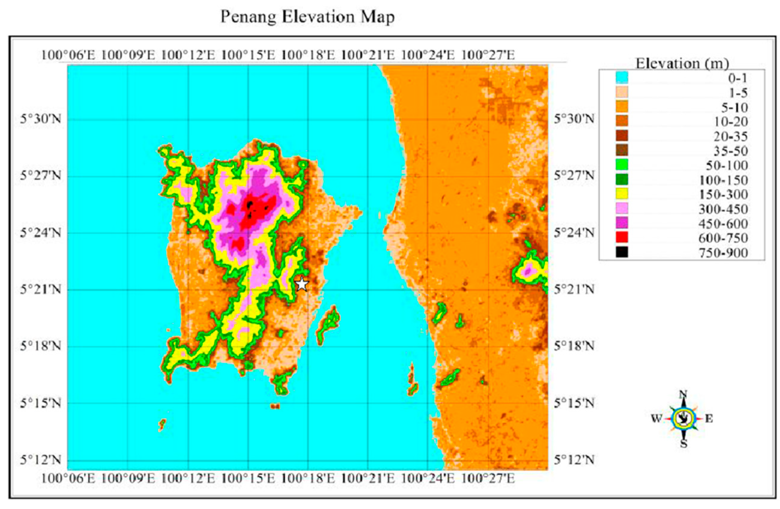
2. Study Area and Atmospheric Dynamics Analysis over the Observational Site

The Raymetrics LB100-ESS-D200 Eye-Safe Scanning Lidar system was deployed for atmospheric studies on the rooftop of the School of Physics building (15 m tall), USM, Pulau Pinang at a latitude of 5.5 N and a longitude of 100.30 E and 10 m above sea level. Pulau Pinang island, located in the north western region of Peninsular Malaysia, lies within latitudes 5.2 N to 5.5 N and longitudes 100.15 E to 100.43 E (Figure 2). The physics building rooftop, 15 m tall, is located south of Georgetown, at about 1.7 km from the eastern shore. Surrounded by the sea of the Straits of Malacca, the island is densely populated, highly urbanized (Georgetown, the main city, counts about 220,000 inhabitants), and industrialized. It is one of the largest and busiest cities in Malaysia.

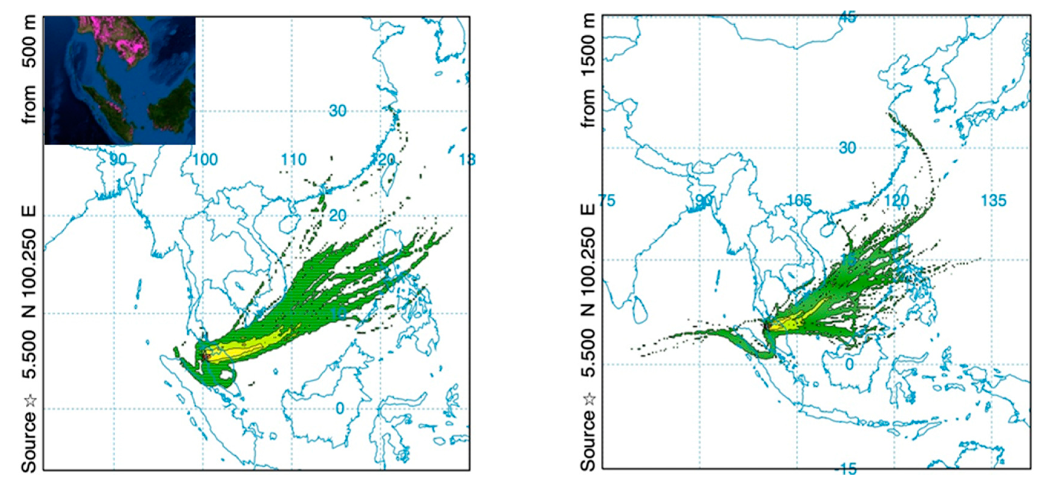
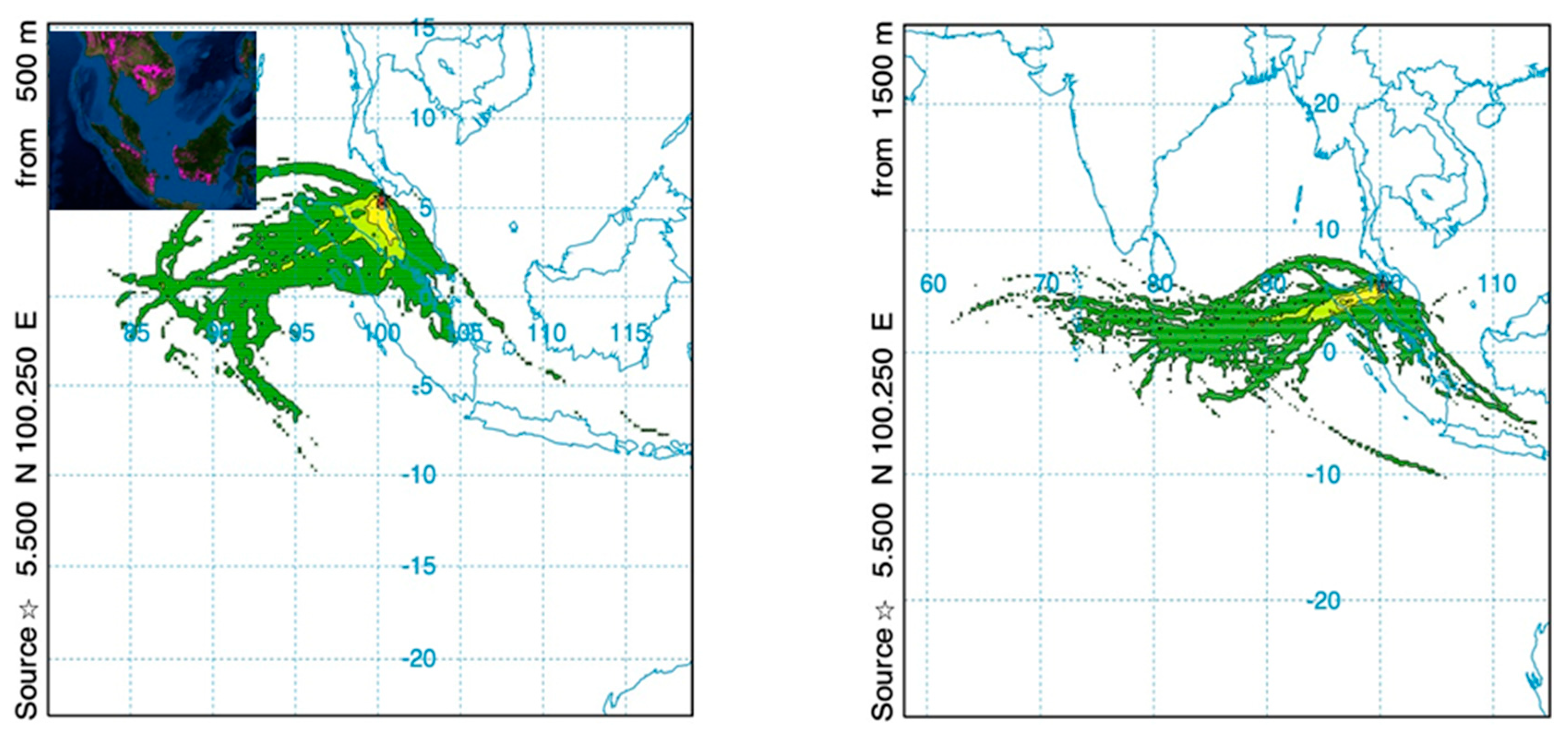
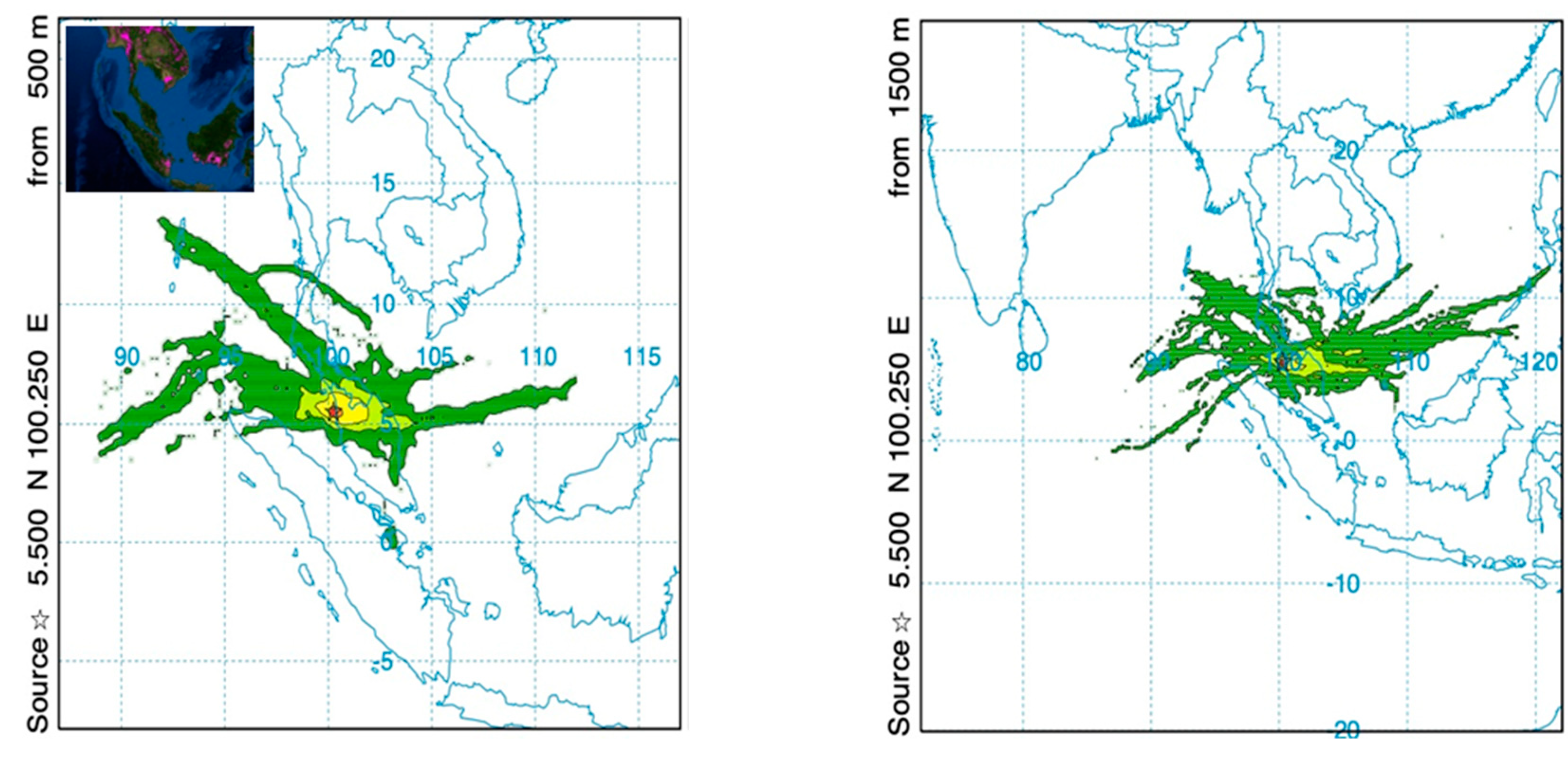
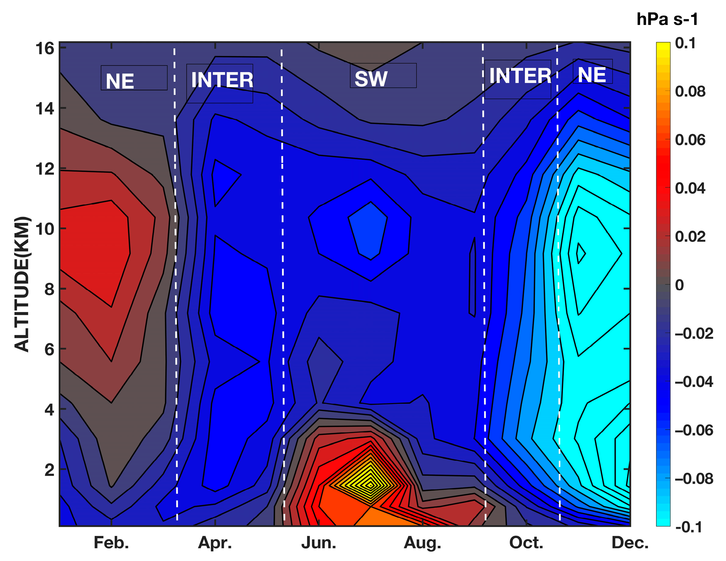
2.1. Back-Trajectory Analysis and Vertical Atmospheric Dynamics at Observational Site

Different spatial and temporal scales influence air quality over Pulau Pinang, an island with many industrial plants leading in manufacturing activities and heavy road traffic with consequent exhaust of aerosol emissions. Surrounded by sea, the background aerosols would likely consist mostly of fine particles, typical of urban environment (road traffic, cooking, and industrial emissions) and marine particles. Due to its particular orography, pollutant transport and dispersion over Penang is subject to microscale atmospheric local circulation, mostly driven by land–water gradients. However, at a temporal scale of a few months, the boundary layer can still be considered, as well mixed, and it is possible to perform an analysis on a synoptical scale to assess how the vertical atmospheric dynamic conditions are favoring atmospheric pollutant build-up [27]. Based on the information from the Malaysian Meteorological Department [28], there are two main monsoon seasons that occur in Malaysia: The Southwest monsoon that begins in late May and ends in September, and the Northeast monsoon that starts blowing from November to March. In April, May, and October (the inter-monsoon months), it is not possible to identify a well-defined strong pattern in blowing winds. During the monsoon seasons, smoke from other remote SEA regions is advected in Pulau Pinang, degrading the air-quality. Figure 3, Figure 4, and Figure 5 show the backward trajectory analysis based on the effective lidar measurement days (139, Section 3.1) obtained from the Hybrid Single-Particle Lagrangian Integrated Trajectory (HYSPLIT; [29]) model, together with the active detected fire hotspots by MODIS. The trajectory patterns clearly trace out a seasonal aerosol advection that depends on the particular season. Penang is downwind of active fire hotspots from November to March and June to September (monsoon seasons), while local background aerosols dominate during the inter-monsoon seasons (April, May, October) [18]. The maximum number of fire hotspots are detected [30] during the southwest monsoon (June to September) [18,19] that coincide with higher aerosol optical depth (AOD). The majority of fire hotspots are detected in southern Peninsular Malaysia, Eastern Sumatra, and Indochina. In other months, a lower number of fire hotspots are detected [31]. From the backward trajectory analysis, it can be observed that during the Northeast (NE) monsoon season, the wind direction at two altitudes (500 m and 1500 m) shows similar patterns. Figure 3 puts in evidence that, before reaching Penang, the air masses transit over Indochina, where a high concentration of fire hotspots are detected (Figure 3 inset, pink spots, form MODIS). During the Southwest (SW) monsoon season, the air masses (especially at 500 m) transit over Sumatra where, again, several fires are active. Being that Sumatra is much closer to the observational site than Indochina, we can speculate that a higher concentration of smoke will be advected towards Penang with respect to the NE monsoon. On the contrary, winds during the inter-monsoon season do not show a pronounced preferred direction, and the back-trajectory analysis puts in evidence that the air masses advected over the observational site transit over regions where fire hotspots are not relevant.
The vertical analysis on atmospheric dynamics at the observational site is based on National Centers for Environmental Prediction/National Center for Atmospheric Research (NCEP/NCAR) reanalysis for 2014. The composite omega value, designating the atmospheric vertical motion, expressed in hPa s−1, is shown in Figure 6. It can be noticed that during the SW monsoon, subsidence is present in the lower troposphere (surface/1.5 km). During the NE monsoon, again, upper air troposphere subsidence is present for January–February–March, while for November–December, air raises in the atmospheric column. During the inter-monsoon season, weak activity is present, corroborating the speculation that the aerosols are not transported from distant regions, but are local.

3. Materials and Methods

3.1. The Raymetrics Lidar

The ground-based lidar deployed at USM of Pulau Penang is a commercial unit, the LB100-ESS-D200, developed by Raymetrics. The laser source emits pulses of wavelength 355 nm (UV) into the atmosphere vertically at zenith. The laser fires 1200 shots per minute (pulse repetition frequency: 20 Hz). The lidar sounds the atmosphere each minute with a spatial vertical resolution of 15 m. Details on the specification of the Raymetrics ground-based Lidar are found in the Table 1.
To avoid instrument damages, a dome equipped with a rain sensor shuts down automatically in case of precipitation. Due to air-traffic safety regulations, the measurements are taken only during working hours, from 8 am to 5 pm local time (from 00UTC to 09UTC), on weekdays. The instrument underwent maintenance (no measurements) the whole month of February and the first half of July. A total of 139 days of data were collected in the year 2014 and processed. Lidar measurement days in 2014 are the following: 8 days in January, 19 days in March, 16 days in April, 19 days in May, 17 days in June, 7 days in July, 10 days in August, 8 days in September, 13 days in October, 12 days in November, and 10 days in December.
The extinction atmospheric profile is retrieved using a classic method described extensively in literature [32,33]. The lidar equation in Equation (1) contains two unknowns, i.e., the aerosol backscattering coefficient and the aerosol extinction coefficient:
P λ ( r ) r 2 = C λ O λ ( r ) [ β m ( r ) + β p ( r ) ] T λ 2 ( r )
where P λ ( r ) r 2 is the range corrected received power, C λ is related to the system calibration coefficient, and T λ 2 ( r ) is the total two-way signal transmission containing the integration of α t o t ( r ) the total extinction coefficient. β m ( r ) and β p ( r ) are the molecular and aerosol backscattering coefficients, respectively. The uncertainties associated with each single variable is described in [34]. O λ ( r ) is the overlap function, and equals unity when the fields of view of the telescope (2.3 mrad) and laser fully overlap (at about r = 450 m). Independent estimations of the lidar overlap function from commercially available Raymetrics lidar model with the same technical specifications and operated under the same configuration are reported in [35]. From the range corrected signal comparison (Figure 3 of [35]), it is clear that the full overlap is reached well below 300 m, in agreement with the observations obtained at Penang. From ground to the full overlap altitude, it is possible to assume a constant extinction value with an acceptable associated error [36].
To invert the signal, it is then necessary to establish a proportionality relation between the extinction and backscattering coefficients: The so-called lidar ratio (LR). LR is a complicated function of size distribution, shape, composition, and refractive index of the aerosols. LR shows a high variability (20 sr–120 sr) [37,38,39] and is not constant with height. With greater spectral complexity comes more advanced means for measuring α and β with multi-spectra lidars. For instance, the combined detection of the elastic backscattered radiation and inelastic backscattering from the Raman roto-vibrational spectrum of nitrogen (or oxygen), using the Raman lidar technique, permits solving Equation (1) without strong assumptions [40]. When the Raman channel is available, then it is possible to measure the extinction and backscattering coefficients independently, and then LR can be directly retrieved. Nevertheless, the Raman channel daytime measurements show a very low signal-to-noise ratio. For this reason, the extinction and backscattering coefficients are retrieved using an iterative method, described exhaustively in [32] and [41]. This method needs also to assume a constant LR, which is, at first, guessed, and then inferred requiring that the lidar AOD, retrieved by integrating the extinction atmospheric coefficient, matches the measured AOD by the co-located AERONET sun photometer [42]. A quantitative analysis on the radiative effect discrepancies driven by the different lidar techniques at the top of the atmosphere (TOA) and surface (SFC) can be found in [43].
From the planetary boundary layer (PBL; [44,45]) analysis, it is not possible to reliably differentiate local from advected aerosol layers. For this reason, we consider that the aerosol profile retrieved by lidar is in one case pure biomass burning and in the other pure urban. The actual profile will be a combination of those two profiles.

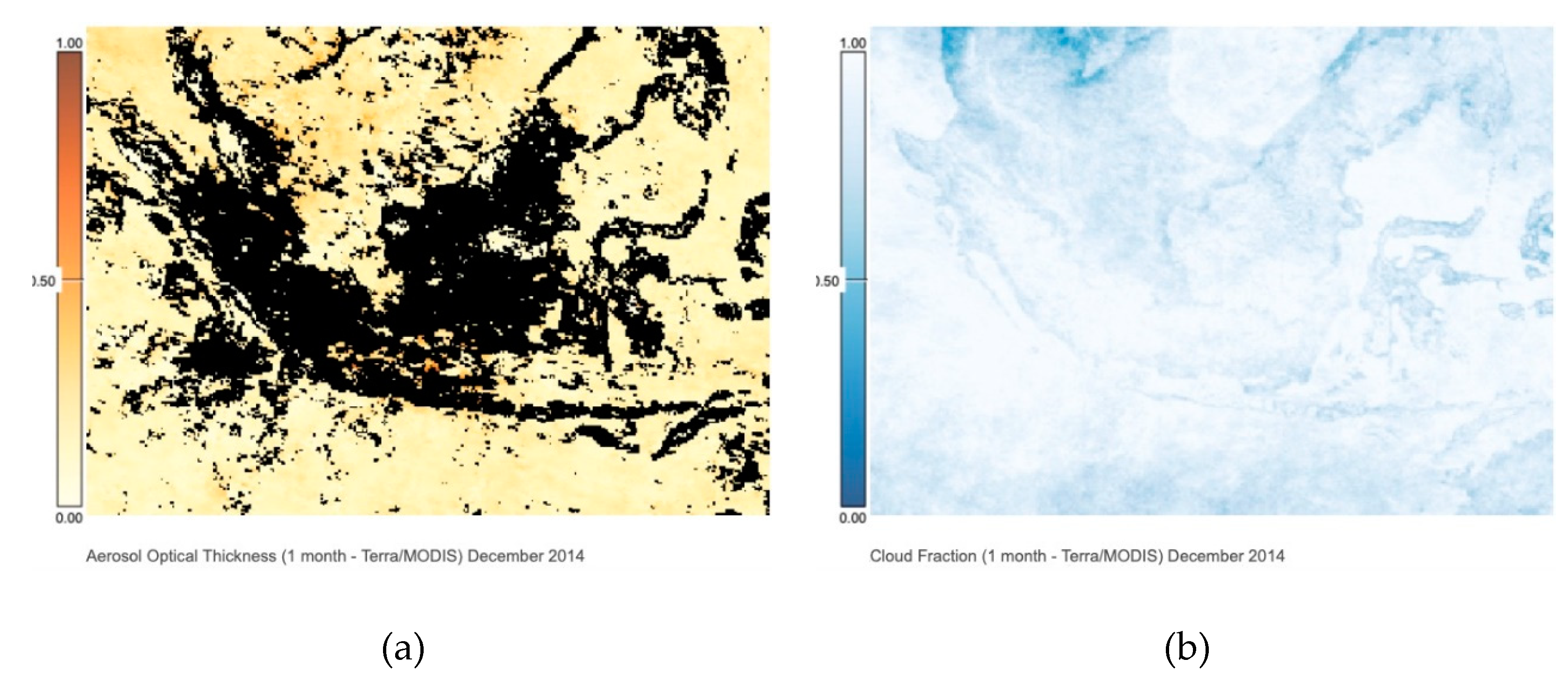
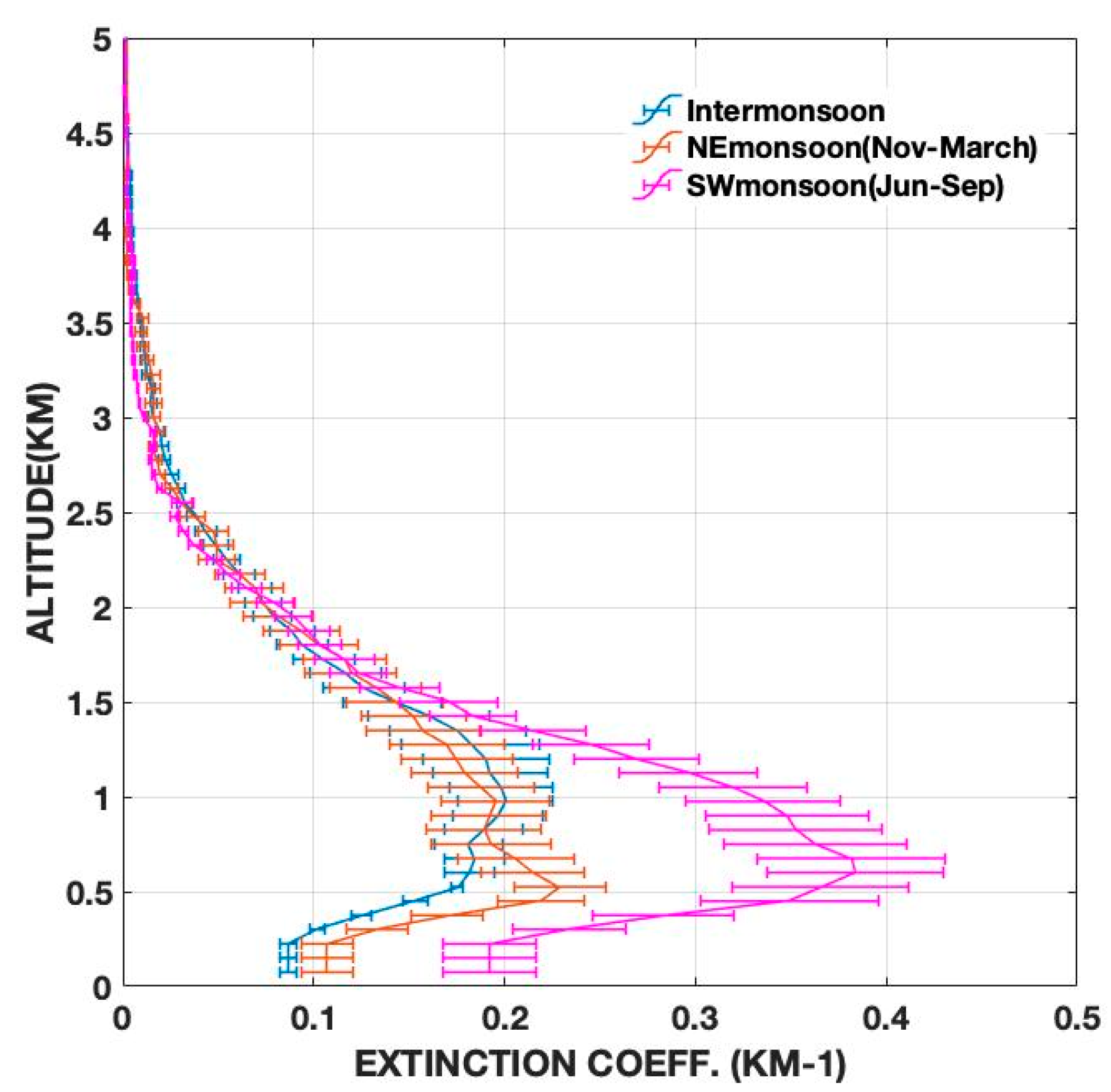
2014 Seasonally Averaged Atmospheric Extinction Coefficients

The daytime atmospheric profiles of the extinction coefficient retrieved with the previously described methodology are averaged over the three different seasons: NE monsoon (November to March), SW monsoon (June to September), and inter-monsoon (April, May, and October). The profiles with relative uncertainty (statistically determined) are shown in Figure 7.
The SW averaged profile shows a higher aerosol loading and a higher AOD (0.52 ± 0.11), confirming what was speculated in Section 2.1. During the NE monsoon season, air masses transit mostly over the ocean and marginally over biomass burning areas. Being the fire hotspot source more distant than during SW monsoon, the AOD is sensibly lower (0.39 ± 0.09) and close to the local background values (see below). During the inter-monsoon season, the aerosol loading reaches the lowest value (AOD = 0.34 ± 0.07). From the seasonally averaged extinction profiles, it can be observed that during the inter-monsoon season, the bulk of the aerosol loading peaks at 1.3 km, shifting towards lower quotes during NW (0.8 km) and SW (0.5 km with a second peak at 1 km). This higher aerosol concentration peak floating over or at the top of the boundary layer has also been observed from the NASA MPLNET lidar network observations during a temporary deployment at USM Penang (not shown here), excluding any possible instrumental artifact, i.e., due to overlap function.

3.2. The Fu–Liou–Gu (FLG) Atmospheric Radiative Transfer Model
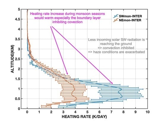
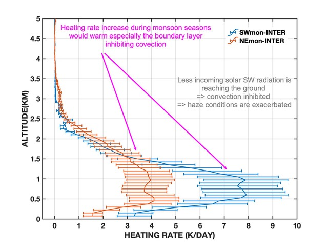
The FLG radiative transfer model [46,47,48,49,50] is used to solve broadband pristine and aerosol (no clouds) radiative fluxes based on seasonally averaged aerosol extinction coefficient profiles (Figure 7), derived from the ground-based lidar observations at USM Penang. The atmosphere thermodynamic parameter profiles, i.e., temperature, humidity, pressure, and gases (i.e., ozone concentration), are obtained from a tropical standard atmosphere (USS976). The aerosol extinction profiles, together with the atmospheric meteorological variables and ozone concentration, are staged as inputs to FLG. The aerosol extinction profiles and, accordingly, the meteorological variables are resolved at 0.075 km resolution from 0 to 30 km above sea level. In the FLG model, the used seasonal mean surface albedo values are obtained from MODIS measurements of the integrated directional hemispherical reflectance [51] near the USM Penang site. Surface albedo values range from 0.11 to 0.14. The surface infrared (IR; 11 μm) emissivity is assumed constant and equal to 0.97. The aerosol parameterization in the FLG radiative transfer model is obtained from the Optical Properties of Aerosol and Clouds (OPAC) catalog [52], where eighteen different aerosol types are available. From air masses analysis, we concluded that the aerosol types over Penang reduce to biomass burning advected from neighbor countries and local urban aerosol types.
Research in [53] highlights that the marine contribution over land is often negligible. This is confirmed by a one-year (2014) analysis performed on aerosol microphysical characteristics using AERONET observation. The analysis puts in evidence that, even if Penang is an island (but very close to the peninsula), the coarser marine aerosol can be neglected when analyzing seasonal averaged data. The observational site is much closer to the eastern shore (1.5 km) with respect to the western open sea (about 12.7 km) from where marine aerosol can be advected. However, the values of the Ångstrom Exponent (AE; 440–870 nm) (1.42 ± 0.11, 1.35 ± 0.15, and 1.53 ± 0.13) Fine Mode Fraction (FMF; 0.84 ± 0.04, 0.78 ± 0.04, 0.73 ± 0.03) and Single Scattering Albedo (SSA; 0.92 ± 0.04, 0.91 ± 0.04, 0.92 ± 0.04) averaged during the three identified seasons (NE, SW, and INTER) exclude, without a doubt, the presence of marine aerosols as reported in [54].

4. Results

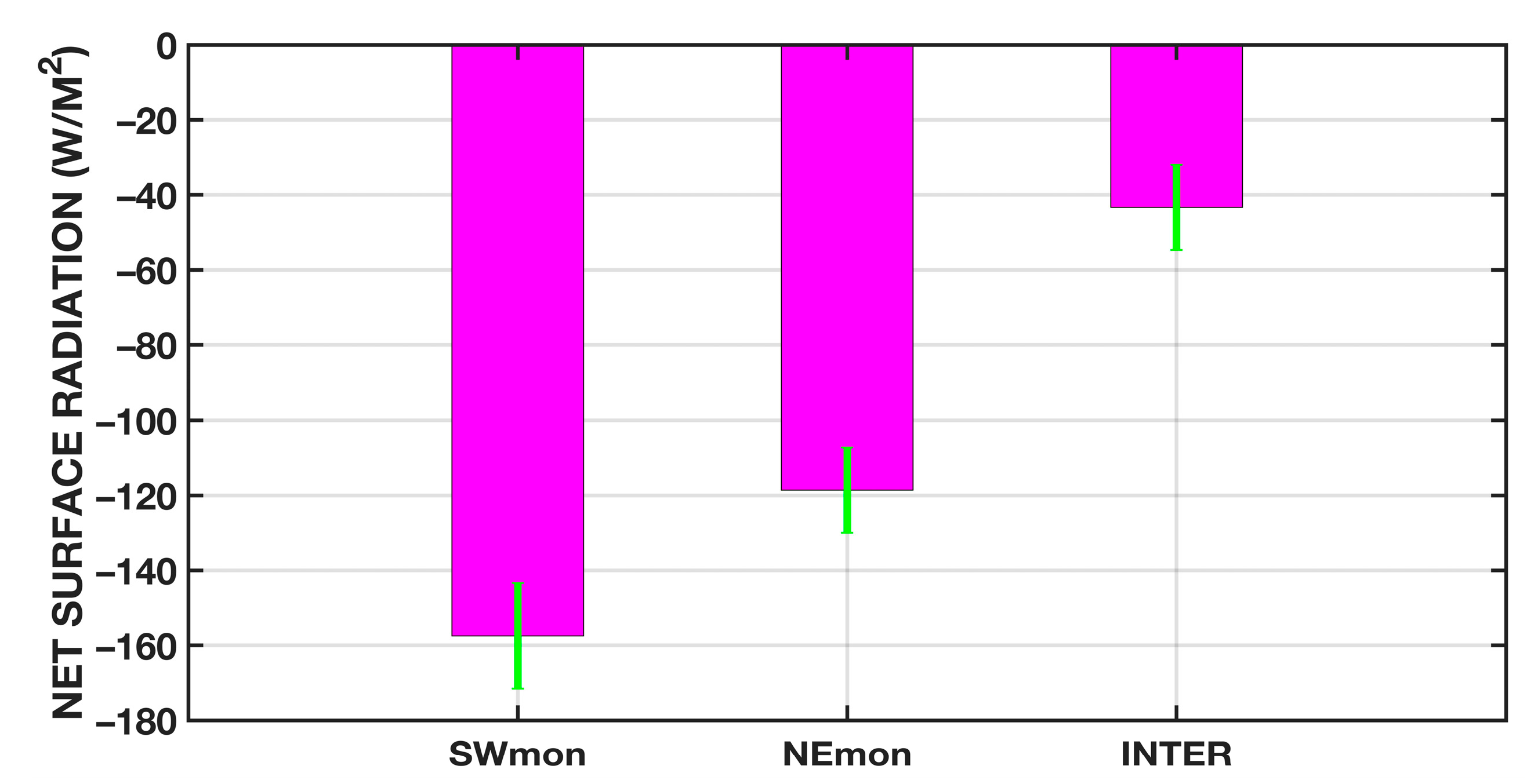
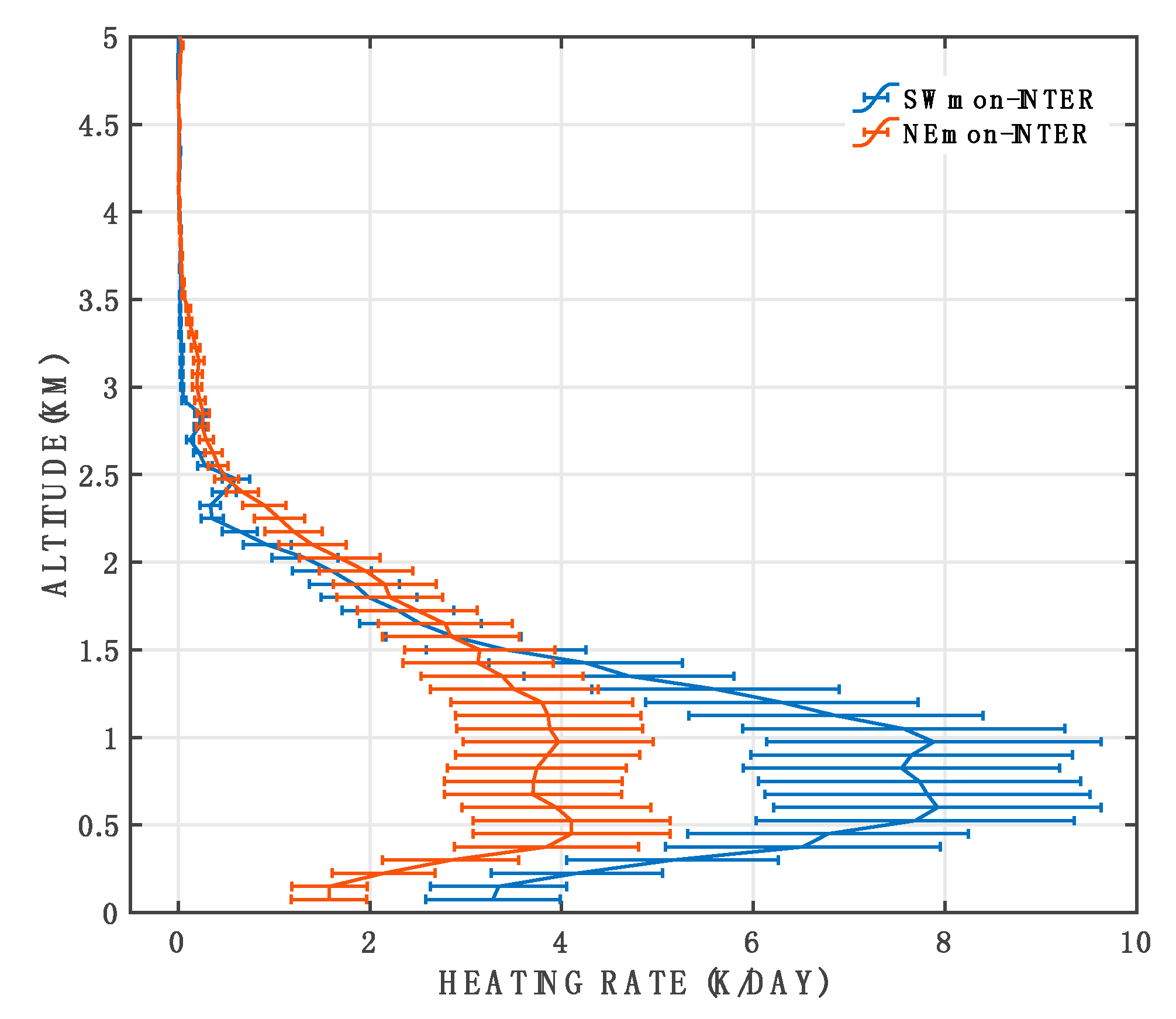
FLG RT Model Results

The FLG radiative transfer model is used to assess the aerosol burden radiative direct effect and column radiative heat differences between monsoon and inter-monsoon seasons [46,47]. As the back-trajectory analysis is not reliable to quantitatively assess how much in percentage the urban and biomass burning aerosol layers distribute into the vertical dimension of the averaged extinction profiles of Figure 7, we computed two distinct runs for the monsoon season considering the atmosphere in turn purely composed by urban and biomass burning aerosols, respectively. For the inter-monsoon season, a run was computed considering only a pure urban aerosol atmosphere. The three (two) surface radiative effect and column heating rate values were averaged together with the extreme values quantifying the variability
To compute the aerosol radiative effect [48,49,50], we averaged over the whole temporal period of each profile of Figure 7 the solar zenith angle, needed as input by the FLG radiative transfer model, at local solar noon to assess the largest aerosol radiative effect. Further we considered tropical standard meteorological conditions, an urban albedo of 0.12 and a surface emissivity of 0.97.
We performed three runs: “Swmon”, “Nemon” and “INTER” (Equation (2)), based on the different averaged aerosol extinction profiles of Figure 7. The radiative effect at the surface is computed for each of the three seasons, subtracting the pristine atmosphere computation, e.g., no clouds, no aerosol, the “TotalSkyAerosol” computation. Clouds were always excluded from the analysis. Cirrus cloud effects were separately analyzed in the region in a previous study, as shown in [15]. Then we computed the aerosol direct radiative effect (DRE), subtracting the results from inter-monsoon computation to SW and NE monsoon seasons, respectively (Equation (4)). To take into account the lidar measurement uncertainty, we ran a Monte Carlo code on the random extinction profile uncertainty to replicate each aerosol extinction profile 30 times. This procedure is explained in detail in [43]. In Equations (2) and (3) are reported how the differences in radiative effect terms are computed among the different seasons:
S W m o n , N E m o n , I N T E R = F L G S W , N E , I N T E R T o t a l S k y A e r o s o l F L G P r i s t i n e
D R E S W = S W m o n I N T E R
D R E N E = N E m o n I N T E R
The analysis puts in evidence that, as shown in Figure 8, during the monsoon seasons, the aerosol burden utterly reduces the energy flux reaching the surface by about 114 and 69 W/m2 for the SW monsoon and the NE monsoon with respect to the inter-monsoon season. Results in Figure 8 are almost totally dominated by the shortwave component of the radiation, as, except for dust that is highly unlikely in the region under study, the effects of aerosol on outgoing longwave radiation are negligible [55]. In Figure 9, we computed the columnar heating rate as the difference between the two monsoon seasons with respect to the inter-monsoon season. The energy not reaching the ground contributes to heat the atmospheric column and especially the first kilometer, with 6.4 K/day and 3.4 K/day for the SW monsoon and the NE monsoon, while in the first 2.5 km, the averaged columnar heating reduces to 4.5 and 2.8 K/day (for the SW monsoon and the NE monsoon, respectively).

5. Discussion

The vertical distribution of aerosol, and especially absorbing aerosols containing black carbon from biomass burning and/or fossil fuels found in Penang Island atmosphere, strongly influence regional and global climate, as shown in [55]. The 2014 case study puts in evidence that the difference in aerosol burden between monsoon and inter-monsoon seasons assessed by paring the Fu–Liou–Gu radiative transfer model with the averaged atmospheric profile of the extinction coefficient obtained from ground-based lidar measurement at USM Penang Malaysia observational site reduces the incoming solar energy flux reaching the Earth surface by 114 and 69 W/m2, respectively (SW and NE monsoons). The aerosols also lead to heating in the first kilometer of 6.4 (SW monsoon) and 3.4 (NE monsoon) K/day. As reported in previous studies [55,56] and confirmed for the first time in this part of the world by ground-based observations, less energy absorption by the Earth surface, combined with PBL warming, leads to increase in the low-level stability during monsoon seasons, with a possible reduction in cloud formation and precipitation. This effect exacerbates the haze episodes with harder dispersion of the advected aerosols.

6. Conclusions

USM Penang ground-based lidar observations during 2014 were used to quantitatively assess the difference in radiative effect and columnar heating rate of the aerosol loading between monsoon (November–March; January–September) and inter-monsoon (April, May and October) seasons. The analysis puts in evidence that, during the monsoon season, on average, the higher aerosol loading prevents 91.5 W/m2 (114–69 W/m2) to reach the ground, while the aerosols are particularly active in warming the first kilometer of the atmosphere of 4.9 K/day (6.4–3.4 W/m2). The showed values were computed at solar noon, therefore these values should be considered as the maximum values. This is the first time that such kind of analysis has been carried, out because continuous ground-based observations are unavailable in the region, while satellite observations are very scarce because of endemic cloudy sky (especially cirrus clouds, up to 70% of the time). Following this preliminary study, in future research topics, we will quantitatively assess the aerosol–cloud radiative effect on the Earth–atmosphere system, considering aerosol layers topped by cirrus clouds. This future research will fill a gap in retrieving radiative effects when satellite retrievals fail. Moreover, other years will be included into the analysis to confirm the observed trend in 2014 and the assessment of how the aerosol loading affects precipitation and cloud lifetime. The obtained results put also in evidence the need of more permanent observation sites across the South-East Asia region.

Author Contributions

Conceptualization, S.L. and W.Y.K.; methodology, S.L.; software, S.L. and W.Y.K.; validation, S.L., W.Y.K., M.Z.M., and H.S.L.; formal analysis, S.L.; investigation, S.L.; resources, M.Z.M. and H.S.L.; data curation, S.L and W.Y.K.; writing—original draft preparation, W.Y.K.; writing—review and editing, S.L.; visualization, W.Y.K.; supervision, H.S.L. and M.Z.M.; project administration, W.Y.K. and H.S.L; funding acquisition, W.Y.K. and H.S.L.

Funding

The financial support by the European Union's Horizon 2020 research and innovation programme (grant agreement No. 654109-project ACTRIS-2 (Aerosols, Clouds, and Trace Gases Research InfraStructure)) is gratefully acknowledged.

Acknowledgments

This project was conducted with financial support from FRGS grant, Investigation of Aerosol Characteristics and Distribution In Malaysia By Using AERONET and Lidar Data, 203/PFIZIK/6711352.

Conflicts of Interest

The authors declare no conflicts of interest.

References

  1. Reid, J.S.; Hyer, E.J.; Johnson, R.S.; Holben, B.N.; Yokelson, R.J.; Zhang, J.; Holz, R.E. Observing and Understanding the Southeast Asian Aerosol System by Remote Sensing: An Initial Review and Analysis for the Seven Southeast Asian Studies (7SEAS) Program. Atmos. Res. 2013, 122, 403–468. [Google Scholar] [CrossRef]
  2. Reid, J.S.; Lagrosas, N.D.; Jonsson, H.H.; Reid, E.A.; Atwood, S.A.; Boyd, T.J.; Ghate, V.P.; Xian, P.; Posselt, D.J.; Simpas, J.B.; et al. Aerosol meteorology of Maritime Continent for the 2012 7SEAS southwest monsoon intensive study—Part 2: Philippine receptor observations of fine-scale aerosol behavior. Atmos. Chem. Phys. 2016, 16, 14057–14078. [Google Scholar] [CrossRef]
  3. Field, R.D.; van der Werf, G.R.; Shen, S.S.P. Human amplification of drought-induced biomass burning in Indonesia since 1960. Nat. Geosci. 2009, 2, 185–188. [Google Scholar] [CrossRef]
  4. Miettinen, J.; Liew, S.C. Degradation and development of peatlands in Peninsular Malaysia and in the islands of Sumatra and Borneo since 1990. Land Degrad. Dev. 2010, 21, 285–296. [Google Scholar] [CrossRef]
  5. Page, S.E.F.; Siegert, J.O.; Rieley, H.D.V.; Boehm, A.; Jaya, S. Limin The amount of carbon released from peat and forest in Indonesia during 1997. Nature 2002, 420, 61–65. [Google Scholar] [CrossRef]
  6. Siegert, G.; Ruecker, A.; Hindrichs, A.A. Hoffmann Increased damage from fires in logged forests during droughts caused by El Niño. Nature 2001, 414, 437–440. [Google Scholar] [CrossRef]
  7. Reid, J.S.; Xian, P.; Hyer, E.J.; Flatau, M.K.; Ramirez, E.M.; Turk, F.J.; Sampson, C.R.; Zhang, C.; Fukada, E.M.; Maloney, E.D. Multi-Scale Meteorological Conceptual Analysis of Observed Active Fire Hotspot Activity and Smoke Optical Depth in the Maritime Continent. Atmos. Chem. Phys. 2012, 12, 2117–2147. [Google Scholar] [CrossRef]
  8. Campbell, J.R.C.; Ge, J.; Wang, E.J.; Welton, A.; Bucholtz, E.J.; Hyer, E.A.; Reid, B.N.; Chew, S.; Liew, S.V.; Salinas, S.; et al. Applying Advanced Ground-Based Remote Sensing in the Southeast Asian Maritime Continent to Characterize Regional Proficiencies in Smoke Transport Modeling. J. Appl. Meteorol. Climatol. 2016, 55, 3–22. [Google Scholar] [CrossRef]
  9. Lolli, S.; Di Girolamo, P. Principal Component Analysis Approach to Evaluate Instrument Performances in Developing a Cost-Effective Reliable Instrument Network for Atmospheric Measurements. J. Atmos. Ocean. Technol. 2015, 32, 1642–1649. [Google Scholar] [CrossRef]
  10. Holben, B.N.; Eck, T.F.; Slutsker, I.; Tanré, D.; Buis, J.P.; Setzer, A.; Vermote, E.; Reagan, J.A.; Kaufman, Y.J.; Nakajima, T.; et al. AERONET—A Federated Instrument Network and Data Archive for Aerosol Characterization. Remote Sens. Environ. 1998, 66, 1–16. [Google Scholar] [CrossRef]
  11. Campbell, J.R.; Hlavka, D.L.; Welton, C.J.; Flynn, E.J.; Turner, D.D.; Spinhirne, J.D.; Scott, V.S.; Hwang, I.H. Aerosol Lidar Observation at Atmospheric Radiation Measurement Program Sites: Instrument and Data Processing. J. Atmos. Ocean. Technol. 2002, 19, 431–442. [Google Scholar] [CrossRef]
  12. Welton, E.J.; Campbell, J.R.; Spinhirne, J.D.; Scott, V.S. Global monitoring of clouds and aerosols using a network of micro-pulse lidar systems. Proc. SPIE 2002, 4153, 151–158. [Google Scholar]
  13. Ciofini, M.; Lapucci, A.; Lolli, S. Diffractive optical components for high power laser beam sampling. J. Opt. A 2003, 5, 186. [Google Scholar] [CrossRef]
  14. Lolli, S.; Delaval, A.; Loth, C.; Garnier, A.; Flamant, P.H. 0.355-micrometer direct detection wind lidar under testing during a field campaign in consideration of ESA’s ADM-Aeolus Mission. Atmos. Meas. Tech. 2013, 6, 3349–3358. [Google Scholar] [CrossRef]
  15. Lolli, S.; Campbell, J.R.; Lewis, J.R.; Gu, Y.; Marquis, J.W.; Chew, B.N.; Liew, S.; Salinas, S.V.; Welton, E.J. Daytime Top-of-the-Atmosphere Cirrus Cloud Radiative Forcing Properties at Singapore. J. Appl. Meteor. Climatol. 2017, 56, 1249–1257. [Google Scholar] [CrossRef]
  16. Raj, P.E.; Devara, P.C.S.; Maheskumar, R.S.; Pandithurai, G.; Dani, K.K. Lidar Measurements of Aerosol Column Content in an Urban Nocturnal Boundary Layer. Atmos. Res. 1997, 45, 201–216. [Google Scholar]
  17. Müller, D.; Mattis, I.; Wandinger, U.; Ansmann, A.; Althausen, D.; Dubovik, O.; Stohl, A. Saharan Dust over a Central European EARLINET-AERONET Site: Combined Observations with Raman Lidar and Sun Photometer. J. Geophys. Res. 2003, 108, 1–17. [Google Scholar] [CrossRef]
  18. Wang, S.H.; Tsay, S.C.; Lin, N.H.; Chang, S.C.; Li, C.; Welton, E.J.; Kuo, C.C. Origin, transport, and vertical distribution of atmospheric pollutants over the northern South China Sea during the 7SEAS/Dongsha experiment. Atmos. Environ. 2012, 78, 124–133. [Google Scholar] [CrossRef]
  19. Pani, S.K.; Wang, S.H.; Lin, N.H.; Tsay, S.C.; Lolli, S.; Chuang, M.T.; Yu, J.Y. Assessment of aerosol optical property and radiative effect for the layer decoupling cases over the northern South China Sea during the 7-SEAS/Dongsha Experiment. J. Geophys. Res. Atmos. 2016, 120. [Google Scholar] [CrossRef]
  20. Tan, F.Y.; Hee, W.S.; Hwee, S.L.; Abdullah, K.; Tiem, L.Y.; Matjafri, M.Z.; Welton, E.J. Variation in daytime tropospheric aerosol via LIDAR and sunphotometer measurements in Penang, Malaysia. AIP Conf. Proc. 2014, 1588, 286–292. [Google Scholar]
  21. Hee, W.S.; San Lim, H.; Jafri, M.Z.M.; Lolli, S.; Ying, K.W. Vertical Profiling of Aerosol Types Observed across Monsoon Seasons with a Raman Lidar in Penang Island, Malay. Aerosol Air Qual. Res. 2016, 16, 2843–2854. [Google Scholar] [CrossRef]
  22. Ding, Y.H.; Lau, N.C.; Johnson, R.H.; Wang, B.; Yasunari, T. The Global Monsoon System: Research and Forecast, 2nd ed.; World Scientific: Singapore, 2011. [Google Scholar]
  23. Hunt, W.H.; Winker, D.M.; Vaughan, M.A.; Powell, K.A.; Lucker, P.L.; Weimer, C. CALIPSO lidar description and performance assessment. J. Atmos. Ocean. Technol. 2009, 26, 1214–1228. [Google Scholar] [CrossRef]
  24. Remer, L.A.; Kaufman, Y.J.; Tanré, D.; Mattoo, S.; Chu, D.A.; Martins, J.V.; Eck, T.F. The MODIS aerosol algorithm, products, and validation. J. Atmos. Sci. 2005, 62, 947–973. [Google Scholar] [CrossRef]
  25. Bilal, M.; Nazeer, M.; Nichol, J.E.; Bleiweiss, M.P.; Qiu, Z.; Jäkel, E.; Lolli, S. A Simplified and Robust Surface Reflectance Estimation Method (SREM) for Use over Diverse Land Surfaces Using Multi-Sensor Data. Remote Sens. 2019, 11, 1344. [Google Scholar] [CrossRef]
  26. Illingworth, A.J.; Barker, H.W.; Beljaars, A.; Ceccaldi, M.; Chepfer, H.; Clerbaux, N.; Fukuda, S. The EarthCARE satellite: The next step forward in global measurements of clouds, aerosols, precipitation, and radiation. Bull. Am. Meteorol. Soc. 2015, 96, 1311–1332. [Google Scholar] [CrossRef]
  27. Dayan, U.; Ricaud, P.; Zbinden, R.; Dulac, F. Atmospheric pollution over the eastern Mediterranean during summer—A review. Atmos. Chem. Phys. 2017, 17, 13233–13263. [Google Scholar] [CrossRef]
  28. Malaysian Meteorological Department. 2013; Monsoon. Available online: http://www.met.gov.my/index.php?option=com_content&task=view&id=69&Itemid=160 (accessed on 19 August 2015).
  29. Draxler, R.R.; Hess, G.D. An Overview of the HYSPLIT_4 Modelling System for Trajectories, Dispersion, and Deposition. Aust. Meteorol. Mag. 1998, 47, 295–308. [Google Scholar]
  30. Bahiyah, N.; Wahid, A.; Latif, M.T.; Suratman, S. Composition and source apportionment of surfactants in atmospheric aerosols of urban and semi-urban areas in Malaysia. Chemosphere 2013, 91, 1508–1516. [Google Scholar]
  31. Hyer, E.J.; Chew, B.N. Aerosol transport model evaluation of an extreme smoke episode in Southeast Asia. Atmos. Environ. 2010, 44, 1422–1427. [Google Scholar] [CrossRef]
  32. Klett, J.D. Stable Analytical Inversion Solution for Processing Lidar Returns. Appl. Opt.. 1981, 20, 211–220. [Google Scholar] [CrossRef]
  33. Fernald, F.G. Analysis of atmospheric lidar observations: Some comments. Appl. Opt. 1984, 23, 652–653. [Google Scholar] [CrossRef] [PubMed]
  34. Lolli, S. Rain Evaporation Rate Estimates from Dual-Wavelength Lidar Measurements and Intercomparison against a Model Analytical Solution. J. Atmos. Ocean. Technol. 2017, 829. [Google Scholar] [CrossRef]
  35. Sannino, A.; Boselli, A.; Sasso, G.; Spinelli, S.; Wang, X. Optimization of the lidar optical design for measurement of the aerosol extinction vertical profile. EPJ Web Conf. 2019, 197, 02006. [Google Scholar] [CrossRef]
  36. Wiegner, M.; Madonna, F.; Binietoglou, I.; Forkel, R.; Gasteiger, J.; Geiß, A.; Pappalardo, G.; Schäfer, K.; Thomas, W. What is the benefit of ceilometers for aerosol remote sensing? An answer from EARLINET. Atmos. Meas. Tech. 2014, 7, 1979–1997. [Google Scholar] [CrossRef]
  37. Ackermann, J. The Extinction-to-Backscatter Ratio of Tropospheric Aerosol: A Numerical Study. J. Atnos. Ocean. Tech. 1998, 15, 1043–1050. [Google Scholar] [CrossRef]
  38. Ferrare, R.A.; Turner, D.D.; Brasseur, L.H.; Feltz, W.F.; Dubovik, O.; Tooman, T.P. Raman lidar measurements of the aerosol extinction-to-backscatter ratio over the Southern Great Plains. J. Geophys. Res. 2001, 106, 20333–20347. [Google Scholar] [CrossRef] [Green Version]
  39. Veselovskii, I.; Whiteman, D.N.; Korenskiy, M.; Suvorina, A.; Pérez-Ramírez, D. Use of rotational Raman measurements in multiwavelength aerosol lidar for evaluation of particle backscattering and extinction. Atmos. Meas. Tech. 2015, 8, 4111–4122. [Google Scholar] [CrossRef] [Green Version]
  40. Albert, A.; Wandinger, U.; Riebesell, M.; Weitkamp, C.; Michaelis, W. Independent measurement of extinction and backscatter profiles in cirrus clouds by using a combined Raman elastic-backscatter lidar. Appl. Opt. 1992, 31, 7113–7131. [Google Scholar]
  41. Di Girolamo, P.; Ambrico, P.F.; Amodeo, A.; Boselli, A.; Pappalardo, G.; Spinelli, N. Aerosol observations by lidar in the nocturnal boundary layer. Appl. Opt. 1999, 38, 4585–4595. [Google Scholar] [CrossRef]
  42. Welton, E.J.; Voss, K.J.; Quinn, P.K.; Flatau, P.J.; Markowicz, K.; Campbell, J.R.; Johnson, J.E. Measurements of aerosol vertical profiles and optical properties during INDOEX 1999 using micropulse lidars. J. Geophys. Res. 2002, 107, 8019. [Google Scholar] [CrossRef]
  43. Lolli, S.; Madonna, F.; Rosoldi, M.; Campbell, J.R.; Welton, E.J.; Lewis, J.R.; Gu, Y.; Pappalardo, G. Impact of varying lidar measurement and data processing techniques in evaluating cirrus cloud and aerosol direct radiative effects. Atmos. Meas. Tech. 2018, 11, 1639–1651. [Google Scholar] [CrossRef] [Green Version]
  44. Haeffelin, F.; Angelini, Y.; Morille, G.; Martucci, S.; Frey, G.P.; Gobbi, S.; Lolli, C.D.; O’Dowd, L.; Sauvage, I.; Xueref-Rémy, B.; et al. Evaluation of Mixing-Height Retrievals from Automatic Profiling Lidars and Ceilometers in View of Future Integrated Networks in Europe. Bound. Layer Meteorol. 2012, 143, 49–75. [Google Scholar] [CrossRef]
  45. Milroy, C.; Martucci, G.; Lolli, S.; Loaec, S.; Sauvage, L.; Xueref-Remy, I.; O’Dowd, C.D. An Assessment of Pseudo-Operational Ground-Based Light Detection and Ranging Sensors to Determine the Boundary-Layer Structure in the Coastal Atmosphere. Adv. Meteorol. 2012, 2012, 929080. [Google Scholar] [CrossRef] [Green Version]
  46. Fu, Q.; Liou, K.N. On the correlated k-distribution method for radiative transfer in nonhomogeneous atmospheres. J. Atmos. Sci. 1992, 49, 2139–2156. [Google Scholar] [CrossRef] [Green Version]
  47. Fu, Q.; Liou, K.N. Parameterization of the radiative properties of cirrus clouds. J. Atmos. Sci. 1993, 50, 2008–2025. [Google Scholar] [CrossRef] [Green Version]
  48. Fu, Q.; Liou, K.N.; Cribb, M.; Charlock, T.P.; Grossman, A. Multiple scattering parameterization in thermal infrared radiative transfer. J. Atmos. Sci. 1997, 54, 2799–2812. [Google Scholar] [CrossRef]
  49. Gu, Y.; Ferrara, J.; Liou, K.N.; Mechoso, C.R. Parameterization of cloud–radiation processes in the UCLA general circulation model. J. Clim. 2003, 16, 3357–3370. [Google Scholar] [CrossRef]
  50. Gu, Y.; Liou, K.N.; Ou, S.C.; Fovell, R. Cirrus cloud simulations using WRF with improved radiation parameterization and increased vertical resolution. J. Geophys. Res. 2011, 116. [Google Scholar] [CrossRef]
  51. Strahler, A.H.; Muller, J.; Lucht, W.; Schaaf, C.; Tsang, T.; Gao, F.; Barnsley, M.J. MODIS BRDF/albedo product: Algorithm theoretical basis document version 5.0. MODIS Doc. 1999, 23, 42–47. [Google Scholar]
  52. Hess, M.; Koepke, P.; Schult, I. Optical properties of aerosols and clouds: The software package OPAC. Bull. Am. Meteorol. Soc. 1998, 79, 831–844. [Google Scholar] [CrossRef]
  53. Bellouin, N.; Quaas, J.-J.; Morcrette, O.B. Estimates of aerosol radiative forcing from the MACC re-analysis. Atmos. Chem. Phys. 2013, 13, 2045–2062. [Google Scholar] [CrossRef] [Green Version]
  54. Mielonen, T.; Arola, A.; Komppula, M.; Kukkonen, J.; Koskinen, J.; De Leeuw, G.; Lehtinen, K.E.J. Comparison of CALIOP level 2 aerosol subtypes to aerosol types derived from AERONET inversion data. Geophys. Res. Lett. 2009, 36. [Google Scholar] [CrossRef]
  55. Johnson, B.T.; Shine, K.P.; Forster, P.M. The semi-direct aerosol effect: Impact of absorbing aerosols on marine stratocumulus. Q. J. R. Meteorol. Soc. 2004, 130, 1407–1422. [Google Scholar] [CrossRef] [Green Version]
  56. Ramanathan, V.C.P.J.; Crutzen, P.J.; Kiehl, J.T.; Rosenfeld, D. Aerosols, climate, and the hydrological cycle. Science 2001, 294, 2119–2124. [Google Scholar] [CrossRef] [PubMed] [Green Version]
Figure 1. MODIS averaged aerosol optical depth (a) during December 2014. Black spots indicate that data are not available because of cloud coverage (close to 100%), as shown on MODIS cloud fraction (b).
Remotesensing 11 02660 g001
Figure 2. Topography of Penang region with elevation in meters. The white star represents the lidar location at Universiti Sains Malaysia.
Remotesensing 11 02660 g002
Figure 3. Monthly backward trajectories density plot (120 hours run time; green 1%, light green 5%, yellow 10%, orange 30%) November to March 2014. HYSPLIT was initialized through the NCEP Global Data Assimilation System (GDAS) with 1 × 1 degree resolution. Inset: MODIS Fire Counts detected in the same period.
Remotesensing 11 02660 g003
Figure 4. Same as Figure 3, but for Southwest monsoon (June–September 2014).
Remotesensing 11 02660 g004
Figure 5. Same a Figure 4, but for the inter-monsoon season (April, May, and October 2014).
Remotesensing 11 02660 g005
Figure 6. NCEP/NCAR reanalysis mean composite omega values at the different levels. Positive values (red) indicate subsidence (air sinking). NE, Northeast; SW, Southwest.
Remotesensing 11 02660 g006
Figure 7. The atmospheric extinction profiles obtained from USM lidar observations during NE monsoon, SW monsoon, and inter-monsoon seasons.
Remotesensing 11 02660 g007
Figure 8. Net surface radiance for the three different seasons (the SW monsoon, the NE monsoon, and the inter-mosoon) at solar noon.
Remotesensing 11 02660 g008
Figure 9. Columnar heating rate difference between monsoon and inter-monsoon seasons. On average, in the first 2.5 km, the averaged heating rate is 4.5 K/day (6.4 K/day in the first kilometer) and 2.8 K/day (3.4 K/day in the first kilometer) for SW and NE, respectively. The effect is then stronger closer to the ground. SWmon, SW monsoon; NEmon, NE monsoon; INTER, inter-monsoon.
Remotesensing 11 02660 g009
Table 1. Lidar instrument technical specifications.
Emitter
Pulsed Laser Source (Class IV Laser) Nd:YAG (Quantel Ultra Series)
Wavelength 355 nm
Energy/Pulse 33.4 mJ
Pulse Duration 5.04 ns
Repetition Rate 20 Hz
Laser Beam Divergence < 0.63 mrad
Near Field Beam Diameter 33.7 mm
Receiver
Telescope Type Cassegrainian
Primary Diameter 200 mm, Parabolic, F10
Secondary Diameter 47 mm diameter, obs: 100 mm
Transmitter–Receiver Distance 162.5 mm
Field of View 1.7 mrad (default, adjustable from 0.5 to 3 mrad)
Interference Filter Bandwidth 1.1 nm @ 355 nm, 1 nm @ 376 nm, 0.88 nm @ 387 nm, 0.97 @ 408 nm
Detection Unit
Transient Recorder LICEL
Detection Channels 2 channels for elastic backscattering 1 channel for Raman backscattering
Detectors 3 PMTs
Detection Mode Analog and photon counting (only photon for 376 nm)
Data Output 2-D time-height cross sections, 3-D temporal evolution of any parameter, ASCII files

