Novel Ensemble of MCDM-Artificial Intelligence Techniques for Groundwater-Potential Mapping in Arid and Semi-Arid Regions (Iran)


Abstract
:
1. Introduction
- Data mining/machine learning models, like boosted regression tree (BRT) [37], classification and regression tree (CART) [38], multivariate adaptive regression splines (MARS) [37], artificial neural network (ANN) [39], random forest (RF) [40], fuzzy logic (FL) [41], Fisher’s linear discriminant function (FLDA) [42], support vector machine (SVM) [43], logistic model tree (LMT) [44], K-nearest neighbor (KNN) [45], and quadratic discriminant analysis [46].
2. Materials and Methods
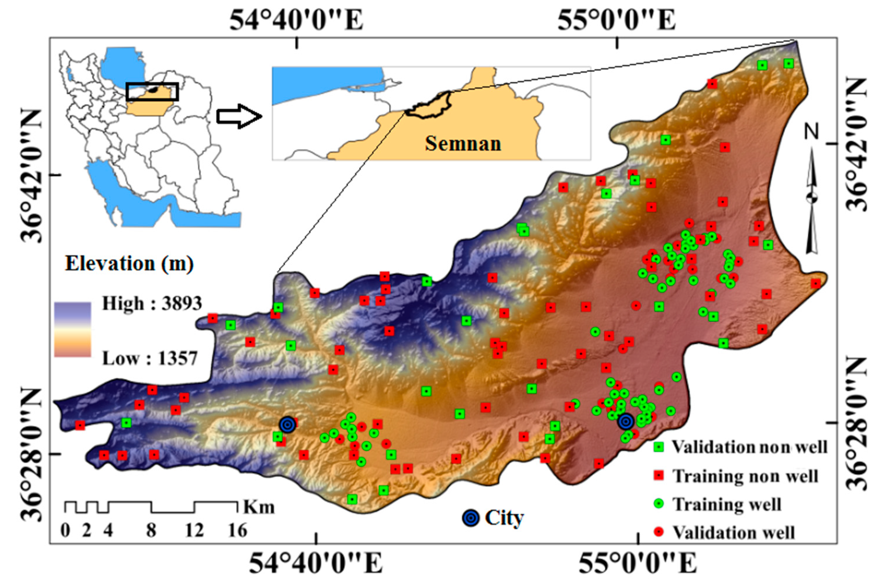
2.1. Study Area
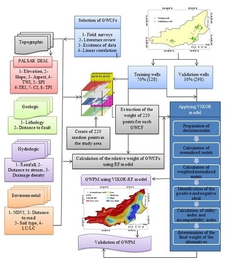
2.2. Methodology
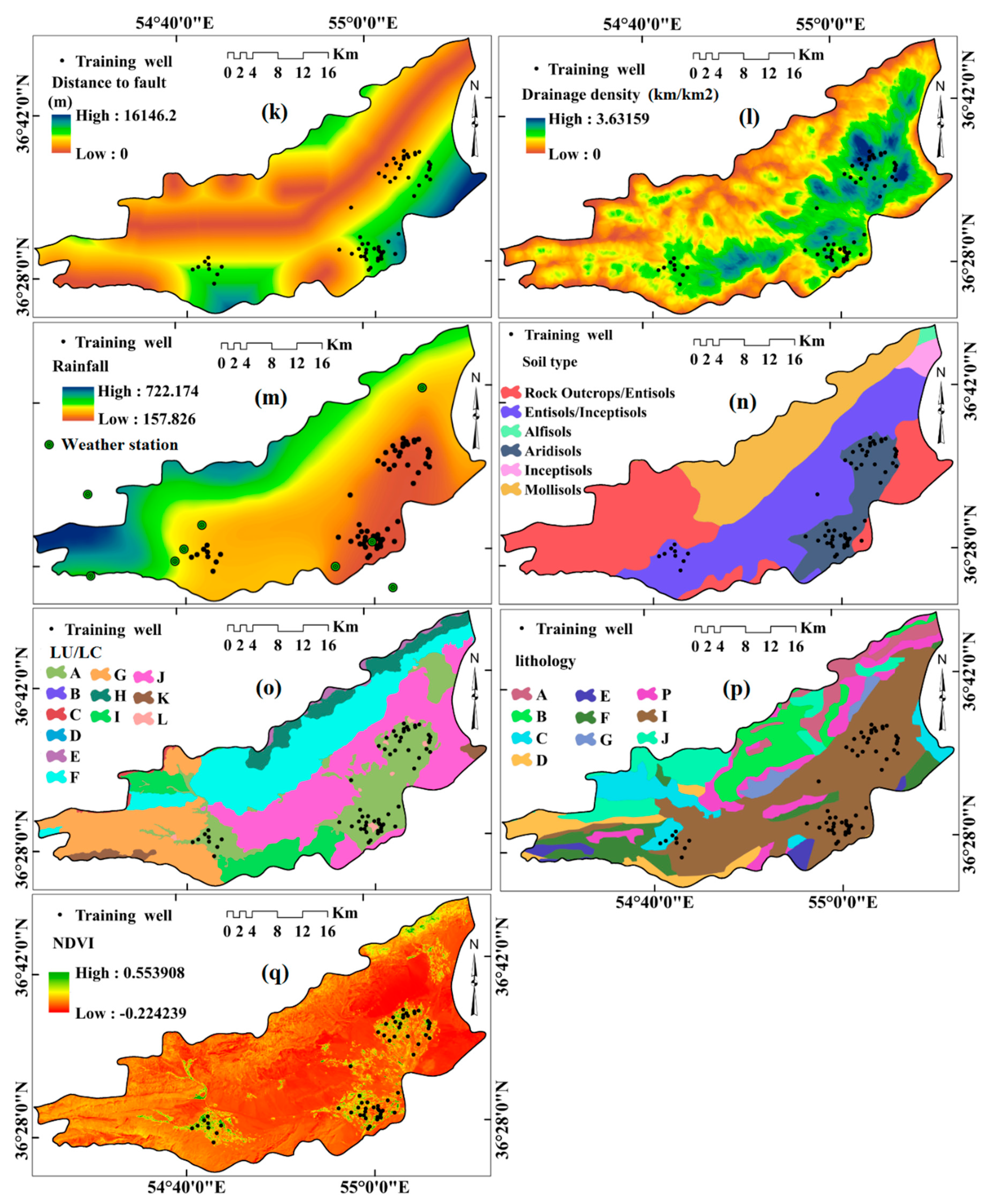
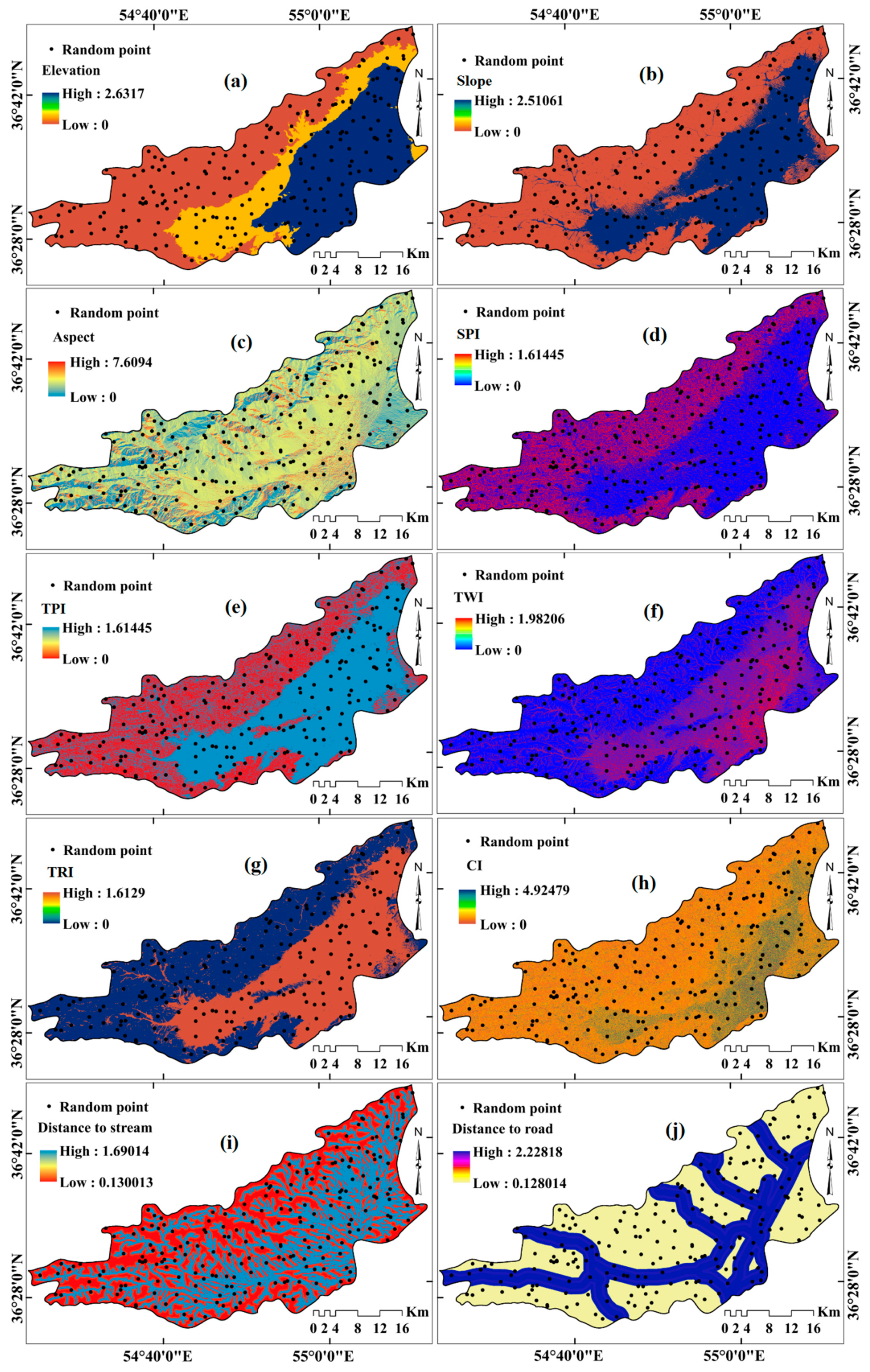
2.3. Data Preparation
2.4. Models
2.4.1. Frequency Ratio (FR)
2.4.2. VIKOR (Vlse Kriterijumsk Optimizacija Kompromisno Resenje)
- (1)
- Prepare the decision matrix.
- (2)
- Calculate the normalized matrix, as shown in Equation (6):where, xij is the ith alternative performance of the jth criterion, and m is the alternative numbers.
- (3)
- Calculate a weighted normalized matrix, as shown in Equation (7):where Wj is the weight of the criterion.
- (4)
- Identify the ideal positive (Equation (8)) and negative (Equation (9)) options:is the positive ideal solution for the ith criterion and is the negative ideal solution for the ith criterion.
- (5)
- Calculate the utility index (Equation (10)) and incompatibility index (the distance from positive and negative ideal solution) (Equation (11)):and are the distance of the ith alternative to the ideal positive and negative solutions, respectively.
- (6)
- Calculate the VIKOR index and determine the final weight of the alternatives, as shown in Equation (12):where V is a constant (0.5), is min Si, is max Si, is min Ri, and is max Ri. The greater the value of the VIKOR index in one alternative, the greater the importance of that alternative.
2.4.3. Random Forest
- ○
- Considers the number of tests (N) and the number of variables (M),
- ○
- Enters R(m) variables to decide on each tree node (m should be less than M),
- ○
- Selects test data for the tree by using the n-times placement of N samples, and the rest of the samples are used to estimate the tree-error,
- ○
- Selects M variables for each tree node, the basis for decision making in each node. The best groups are calculated on m variables in the test-sample, and
- ○
- Expands each tree completely without pruning.
2.5. Validation of Results
3. Results
3.1. Multi-Collinearity Analysis
3.2. Determining the Relative Importance of GWCFs using the RF Model
3.3. Determining the Value of Each Pixel of GWCFs using the FR Model
3.4. Application of VIKOR Model
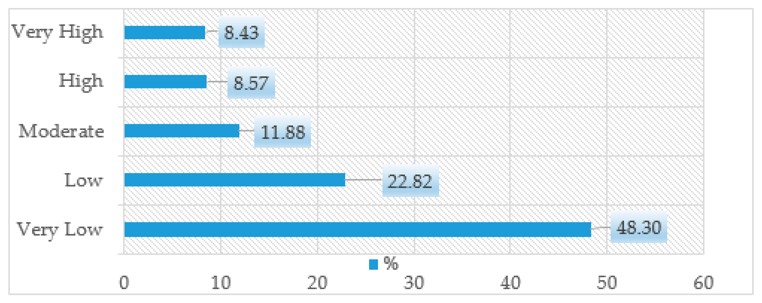
3.5. Groundwater Potential Mapping Using the FR-RF-VIKOR Ensemble Model
3.6. Validation of Results
4. Discussion
5. Conclusions
Author Contributions
Funding
Acknowledgments
Conflicts of Interest
References
- Arabameri, A.; Rezaei, K.; Cerda, A.; Lombardo, L.; Rodrigo-Comino, J. GIS-based groundwater potential mapping in Shahroud plain, Iran. A comparison among statistical (bivariate and multivariate), data mining and MCDM approaches. Sci. Total Environ. 2019, 658, 160–177. [Google Scholar] [CrossRef]
- Foster, S. Groundwater assessing vulnerability and promoting protection of a threatened resource. In Proceedings of the 8th Stockholm Water Symposium, Stockholm, Sweden, 10–13 August 1998. [Google Scholar]
- UN. Water for people, water for life. In The UN World Water Development Report (WWDR), UNESCO; Publishing and Berghahn Books: New York, NY, USA, 2003; p. 34. [Google Scholar]
- ElNaqa, A.; AlShayeb, A. Groundwater protection and management strategy in jordan. Water Resour. Manag. 2008, 23, 2379–2394. [Google Scholar] [CrossRef]
- Schematization and Management Organ of Iran (SMOI). 2004. Available online: http://www.ncc.org.ir/ (accessed on 12 August 2018).
- Magesh, N.S.; Chandrasekar, N.; John, P. Delineation of groundwater potential zones in Theni district, Tamil Nadu, using remote sensing, GIS and MIF techniques. Geosci. Front. 2012, 3, 189–196. [Google Scholar] [CrossRef] [Green Version]
- Lee, S.; Hyun, Y.; Lee, M.J. Groundwater Potential Mapping Using Data Mining Models of Big Data Analysis in Goyang-si, South Korea. Sustainability 2019, 11, 1678. [Google Scholar] [CrossRef] [Green Version]
- Rahmati, O.; Pourghasemi, H.R.; Melesse, A.M.N. Application of GIS-based data driven random forest and maximum entropy models for groundwater potential mapping: A case study at Mehran region, Iran. Catena 2016, 137, 360–372. [Google Scholar] [CrossRef]
- Agarwal, R.; Garg, P.K. Remote Sensing and GIS Based Groundwater Potential & Recharge Zones Mapping Using Multi Criteria Decision Making Technique. Water Resour. Manag. 2016, 30, 243–260. [Google Scholar]
- Mondal, S. Remote sensing and GIS based ground water potential mapping of kangshabati irrigation command area, west bengal. Geogr. Nat. Disasters 2012, 1, 1–8. [Google Scholar] [CrossRef]
- Oikonomidis, D.; Dimogianni, S.; Kazakis, N.; Voudouris, K. A GIS/Remote Sensing-based methodology for groundwater potentiality assessment in Tirnavos area, Greece. J. Hydrol. 2015, 525, 197–208. [Google Scholar] [CrossRef]
- Thomas, A.; Sharma, P.K.; Sharma, M.K.; Sood, A. Hydrogeomorphological mapping in assessing groundwater by using remote sensing datada case study in Lehra Gage Block, Sangrur district, Punjab. J. Indian Soc. Remote Sens. 1999, 27, 31–42. [Google Scholar] [CrossRef]
- Muralidhar, M.; Raju, K.R.K.; Raju, K.S.V.P.; Prasad, J.R. Remote sensing applications for the evaluation of water resources in rainfed area, Warangal district, Andhra Pradesh. Indian Miner. 2003, 34, 33–40. [Google Scholar]
- Pinto, D.; Shrestha, S.; Babel, M.S.; Ninsawat, S. Delineation of groundwater potential zones in the Comoro watershed, Timor Leste using GIS, remote sensing and analytic hierarchy process (AHP) technique. Appl. Water Sci. 2017, 7, 503–519. [Google Scholar] [CrossRef] [Green Version]
- Magaia, L.A.; Goto, T.N.; Masoud, A.A.; Koike, K. Identifying groundwater potential in crystalline basement rocks using remote sensing and electromagnetic sounding techniques in Central Western Mozambique. Nat. Resour. Res. 2018, 27, 275–298. [Google Scholar] [CrossRef]
- Luís, A.M. Development of Regional Exploration Techniques for Groundwater Resources in Semiarid Areas Through Integration of Remote Sensing and Geophysical Survey. Ph.D. Thesis, Kyoto University, Kyoto, Japan, 2018. [Google Scholar]
- Pradhan, B. Groundwater potential zonation for basaltic watersheds using satellite remote sensing data and GIS techniques. Open Geosci. 2009, 1, 120–129. [Google Scholar] [CrossRef]
- Bera, K.; Bandyopadhyay, J. Ground water potential mapping in Dulung watershed using remote sensing & GIS techniques, West Bengal, India. Int. J. Sci. Res. Publ. 2012, 2, 1–7. [Google Scholar]
- Al-Ruzouq, R.; Shanableh, A.; Merabtene, T.; Siddique, M.; Khalil, M.A.; Idris, A.; Almulla, E. Potential groundwater zone mapping based on geo-hydrological considerations and multi-criteria spatial analysis: North UAE. CATENA 2019, 173, 511–524. [Google Scholar] [CrossRef]
- Shi, Z.H.; Cai, C.F.; Ding, S.W.; Wang, T.W.; Chow, T.L. Soil conservation planning at the small watershed level using RUSLE with GIS: A case study in the Three Gorge area of China. Catena 2004, 55, 33–48. [Google Scholar] [CrossRef]
- Sharma, S.; Kumar Mahajan, A. Comparative evaluation of GIS-based landslide susceptibility mapping using statistical and heuristic approach for Dharamshala region of Kangra Valley, India. Geoenviron. Disasters 2018, 5, 4. [Google Scholar] [CrossRef] [Green Version]
- Saro, L. Current and future status of GIS-based landslide susceptibility mapping: A literature review. Korea J. Remote Sens. 2019, 35, 179–193. [Google Scholar]
- Saro, L.; Oh, H.J. Landslide Susceptibility Prediction using Evidential Belief Function, Weight of Evidence and Artificial Neural Network Models. Korea J. Remote Sens. 2019, 35, 299–316. [Google Scholar]
- Arabameri, A.; Pourghasemi, H.R.; Yamani, M. Applying different scenarios for landslide spatial modeling using computational intelligence methods. Environ. Earth Sci. 2017, 76, 832. [Google Scholar] [CrossRef]
- Singh, S.K.; Srivastava, K.; Gupta, M.; Thakur, K.; Mukherjee, S. Appraisal of land use/land cover of mangrove forest ecosystem using support vector machine. Environ. Earth Sci. 2014, 71, 2245–2255. [Google Scholar] [CrossRef]
- Mahato, S.; Pal, S. Groundwater Potential Mapping in a Rural River Basin by Union (OR) and Intersection (AND) of Four Multi-criteria Decision-Making Models. Nat. Resour. Res. 2019, 28, 523–545. [Google Scholar] [CrossRef]
- Lee, S.; Kim, Y.S.; Oh, H.J. Application of a weights of evidence method and GIS to regional groundwater productivity potential mapping. J. Environ. Manag. 2012, 96, 91–105. [Google Scholar] [CrossRef] [PubMed]
- Park, I.; Kim, Y.; Lee, S. Groundwater productivity potential mapping using evidential belief function. Groundwater 2014, 52, 201–207. [Google Scholar] [CrossRef]
- Mogaji, K.A.; Omosuyi, G.O.; Adelusi, A.O.; Lim, H.S. Application of GIS-based evidential belief function model to regional groundwater recharge potential zones mapping in hardrock geologic terrain. Environ. Process. 2016, 3, 93–123. [Google Scholar] [CrossRef]
- Kordestani, M.D.; Naghibi, S.A.; Hashemi, H.; Ahmadi, K.; Kalantar, B.; Pradhan, B. Groundwater potential mapping using a novel data-mining ensemble model. Hydrogeol. J. 2019, 27, 211–224. [Google Scholar] [CrossRef] [Green Version]
- Naghibi, S.A.; Pourghasemi, H.R.; Pourtaghie, Z.S.; Rezaei, A. Groundwater qanat potential mapping using frequency ratio and Shannon’s entropy models in the Moghan Watershed, Iran. Earth Sci. Inf. 2015, 8, 171–186. [Google Scholar] [CrossRef]
- Golkarian, A.; Naghibi, S.A.; Kalantar, B.; Pradhan, B. Groundwater potential mapping using C5.0, random forest, and multivariate adaptive regression spline models in GIS. Environ. Monit. Assess. 2018, 190, 149. [Google Scholar] [CrossRef]
- Trabelsi, F.; Lee, S.; Khlifi, S.; Arfaoui, A. Frequency Ratio Model for Mapping Groundwater Potential Zones Using GIS and Remote Sensing; Medjerda Watershed Tunisia. In Advances in Sustainable and Environmental Hydrology, Hydrogeology, Hydrochemistry and Water Resources; Chaminé, H., Barbieri, M., Eds.; Springer: Berlin/Heidelberg, Germany, 2019. [Google Scholar]
- Razandi, Y.; Pourghasemi, H.R.; SamaniNeisani, N.; Rahmati, O. Application of analytical hierarchy process, frequency ratio, and certainty factor models for groundwater potential mapping using GIS. Earth Sci. Inf. 2015, 8, 867–883. [Google Scholar] [CrossRef]
- Chen, W.; Li, H.; Hou, E.; Wang, S.; Wang, G.; Panahi, M. GIS-based groundwater potential analysis using novel ensemble weights-of-evidence with logistic regression and functional tree models. Sci. Total Environ. 2018, 1, 853–867. [Google Scholar] [CrossRef] [Green Version]
- Lee, S.; Lee, C.W.; Kim, J.C. Groundwater Productivity Potential Mapping Using Logistic Regression and Boosted Tree Models: The Case of Okcheon City in Korea. In Advances in Remote Sensing and Geo Informatics Applications; El-Askary, H., Lee, S., Eds.; Springer: Berlin/Heidelberg, Germany, 2019. [Google Scholar]
- Golkarian, A.; Rahmati, O. Use of a maximum entropy model to identify the key factors that influence groundwater availability on the Gonabad Plain, Iran. Environ. Earth Sci. 2018, 77, 369. [Google Scholar] [CrossRef]
- Naghibi, S.A.; Pourghasemi, H.R.; Dixon, B. GIS-based groundwater potential mapping using boosted regression tree, classification and regression tree, and random forest machine learning models in Iran. Environ. Monit. Assess. 2016, 188, 44. [Google Scholar] [CrossRef] [PubMed]
- Lee, S.; Song, K.Y.; Kim, Y.; Park, I. Regional groundwater productivity potential mapping using a geographic information system (GIS) based artificial neural network model. Hydrogeol. J. 2012, 20, 1511–1527. [Google Scholar] [CrossRef]
- Miraki, S.; Hedayati Zanganeh, S.; Chapi, K.; Singh, V.P.; Shirzadi, A.; Shahabi, H.; Thai Pham, B. Mapping Groundwater Potential Using a Novel Hybrid Intelligence Approach. Water Resour. Manag. 2019, 33, 281–302. [Google Scholar] [CrossRef]
- Shahid, S.; Nath, S.K.; Kamal, A.S. GIS integration of remote sensing and topographic data using fuzzy logic for ground water assessment in Midnapur district, India. Geocarto Int. 2014, 17, 69–74. [Google Scholar] [CrossRef]
- Chen, W.; Pradhan, B.; Li, S.; Shahabi, H.; Mojaddadi Rizeei, H.; Hou, E.; Wang, S. Novel Hybrid Integration Approach of Bagging-Based Fisher’s Linear Discriminant Function for Groundwater Potential Analysis. Nat. Resour. Res. 2019, 28, 1239–1258. [Google Scholar] [CrossRef] [Green Version]
- Naghibi, S.A.; Ahmadi, K.; Daneshi, A. Application of support vector machine, random forest, and genetic algorithm optimized randomforest models in groundwater potential mapping. Water Resour. Manag. 2017, 31, 2761–2775. [Google Scholar] [CrossRef]
- Rahmati, O.; Naghibi, S.A.; Shahabi, H.; Tien Bui, D.; Pradhan, B.; Aareh, A. Groundwater spring potential modelling: Comprising the capability and robustness of three different modeling approaches. Hydrology 2018, 565, 248–261. [Google Scholar] [CrossRef]
- Naghibi, S.A.; Pourghasemi, H.R.; Abbaspour, K. A comparison between ten advanced and soft computing models for groundwater qanat potential assessment in Iran using R and GIS. Theor. Appl. Clim. 2018, 131, 967–984. [Google Scholar] [CrossRef]
- Naghibi, S.A.; Dashtpagerdi, M.M. Evaluation of four supervised learning methods for groundwater spring potential mapping in Khalkhal region (Iran) using GIS-based features. Hydrogeol. J. 2017, 25, 169–189. [Google Scholar] [CrossRef]
- Naghibi, S.A.; Moghaddam, D.D.; Kalantar, B.; Pradhan, B.; Kisi, O. A comparative assessment of GIS-based data mining models and a novel ensemble model in groundwater well potential mapping. J. Hydrol. 2017, 548, 471–483. [Google Scholar] [CrossRef]
- Razavi-Termeh, S.V.; Sadeghi-Niaraki, A.; Choi, S.-M. Groundwater Potential Mapping Using an Integrated Ensemble of Three Bivariate Statistical Models with Random Forest and Logistic Model Tree Models. Water 2019, 11, 1596. [Google Scholar] [CrossRef] [Green Version]
- Alganci, U.; Besol, B.; Sertel, E. Accuracy Assessment of Different Digital Surface Models. ISPRS Int. J. Geo Inf. 2018, 7, 114. [Google Scholar] [CrossRef] [Green Version]
- Arabameri, A.; Pourghasemi, H.R.; Cerda, A. Erodibility prioritization of sub-watersheds using morphometric parameters analysis and its mapping: A comparison among TOPSIS, VIKOR, SAW, and CF multi-criteria decision making models. Sci. Total Environ. 2017, 613, 1385–1400. [Google Scholar]
- Arabameri, A.; Pradhan, B.; Rezaei, K.; Yamani, M.; Pourghasemi, H.R.; Lombardo, L. Spatial modelling of gully erosion using Evidential Belief Function, Logistic Regression and a new ensemble EBF–LR algorithm. Land Degrad. Dev. 2018, 29, 4035–4049. [Google Scholar] [CrossRef]
- Arabameri, A.; Rezaei, K.; Pourghasemi, H.R.; Lee, S.; Yamani, M. GIS-based gully erosion susceptibility mapping: A comparison among three data-driven models and AHP knowledge-based technique. Environ. Earth Sci. 2018, 77, 628. [Google Scholar] [CrossRef]
- Arabameri, A.; Pradhan, B.; Pourghasemi, H.R.; Rezaei, K. Identification of erosion-prone areas using different multi-criteria decision-making techniques and GIS. Geomat. Nat. Hazards Risk 2018, 9, 1129–1155. [Google Scholar] [CrossRef] [Green Version]
- Arabameri, A.; Rezaei, K.; Cerda, A.; Conoscenti, C.; Kalantari, Z. A comparison of statistical methods and multi-criteria decision making to map flood hazard susceptibility in Northern Iran. Sci. Total Environ. 2019, 660, 443–458. [Google Scholar] [CrossRef]
- Arabameri, A.; Pradhan, B.; Rezaei, K.; Conoscenti, C. Gully erosion susceptibility mapping using GIS-based multi-criteria decision analysis techniques. CATENA 2019, 180, 282–297. [Google Scholar] [CrossRef]
- Arabameri, A. Application of the Analytic Hierarchy Process (AHP) for locating fire stations: Case Study Maku City. Merit Res. J. ArtSoc. Sci. Humanit. 2014, 2, 1–10. [Google Scholar]
- Arabameri, A.; Ramesht, M.H. Site Selection of Landfill with emphasis on Hydrogeomorphological–environmental parameters Shahrood-Bastam watershed. Sci. J. Manag. Syst. 2017, 16, 55–80. [Google Scholar]
- Yamani, M.; Arabameri, A. Comparison and evaluation of three methods of multi attribute decision making methods in choosing the best plant species for environmental management (Case study: Chah Jam Erg). Nat. Environ. Chang. 2015, 1, 49–62. [Google Scholar]
- Arabameri, A. Zoning Mashhad Watershed for Artificial Recharge of Underground Aquifers Using Topsis Model and GIS Technique. Glob. J. Hum. Soc. Sci. B Geogr. Geo Sci. Environ. Disaster Manag. 2014, 14, 45–53. [Google Scholar]
- Mousavi, S.M.; Golkarian, A.; Naghibi, S.A.; Kalantar, B.; Pradhan, B. GIS-based groundwater spring potential mapping using data mining boosted regression tree and probabilistic frequency ratio models in Iran. Aims Geosci. 2017, 3, 91–115. [Google Scholar]
- Siahkamari, S.; Haghizadeh, A.; Zeinivand, H.; Tahmasebipour, N.; Rahmati, O. Spatial prediction of flood-susceptible areas using frequency ratio and maximum entropy models. Geocarto Int. 2018, 33, 927–941. [Google Scholar] [CrossRef]
- Arabameri, A.; Pradhan, B.; Rezaei, K.; Sohrabi, M.; Kalantari, Z. GIS-based landslide susceptibility mapping using numerical risk factor bivariate model and its ensemble with linear multivariate regression and boosted regression tree algorithms. J. Mt. Sci. 2019, 16, 595–618. [Google Scholar] [CrossRef]
- Arabameri, A.; Pradhan, B.; Rezaei, K.; Saro, L.; Sohrabi, M. An Ensemble Model for Landslide Susceptibility Mapping in a Forested Area. Geocarto Int. 2019, 1–26. [Google Scholar] [CrossRef]
- Arabameri, A.; Pradhan, B.; Rezaei, K. Spatial prediction of gully erosion using ALOS PALSAR data and ensemble bivariate and data mining models. Geosci. J. 2019, 24, 669–686. [Google Scholar] [CrossRef]
- Arabameri, A.; Pradhan, B.; Rezaei, K.; Lee, C.-W. Assessment of Landslide Susceptibility Using Statistical- and Artificial Intelligence-Based FR–RF Integrated Model and Multiresolution DEMs. Remote Sens. 2019, 11, 999. [Google Scholar] [CrossRef] [Green Version]
- Arabameri, A.; Pradhan, B.; Pourghasemi, H.R.; Rezaei, K.; Kerle, N. Spatial Modelling of Gully Erosion Using GIS and R Programing: A Comparison among Three Data Mining Algorithms. Appl. Sci. 2018, 8, 1369. [Google Scholar] [CrossRef] [Green Version]
- Arabameri, A.; Pourghasemi, H.R. Spatial Modeling of Gully Erosion Using Linear and Quadratic Discriminant Analyses in GIS and R. In Spatial Modeling in GIS and R for Earth and Environmental Sciences, 1st ed.; Pourghasemi, H.R., Gokceoglu, C., Eds.; Elsevier: Amsterdam, The Netherlands, 2019; p. 796. [Google Scholar]
- Arabameri, A.; Pradhan, B.; Rezaei, K. Gully erosion zonation mapping using integrated geographically weighted regression with certainty factor and random forest models in GIS. J. Environ. Manag. 2019, 232, 928–942. [Google Scholar] [CrossRef]
- IRIMO. Summary Reports of Iran’s Extreme Climatic Events. In Ministry of Roads and Urban Development; Iran Meteorological Organization: Tehran, Iran, 2012; Available online: http://www.cri.ac.ir (accessed on 12 August 2018).
- GSI. Geology Survey of Iran. 1997. Available online: http://www.gsi.ir/Main/Lang_en/index.html (accessed on 12 August 2018).
- IUSSWorking Group WRB14. World Reference Base for Soil Resources 2014, World Soil Resources Report; FAO: Rome, Italy, 2014. [Google Scholar]
- Noor, H. Analysis of Groundwater Resource Utilization and Their Current Condition in Iran. Iran. J. Rainwater Catchment Syst. 2018, 5, 29–38. [Google Scholar]
- Ramesht, M.H.; Arabameri, A. Shahrood-Bastam Basin Zoning for the Purpose of Artificial Underground Aquifer Recharge by Using Linear Assignment Method and GIS Technique. Geogr. Space 2013, 12, 134–149. [Google Scholar]
- Chen, W.; Xie, X.; Wang, J.; Pradhan, B.; Hong, H.; Bui, D.T. A comparative study of logistic model tree, random forest, and classification and regression tree models for spatial prediction of landslide susceptibility. Catena 2017, 151, 147–160. [Google Scholar] [CrossRef] [Green Version]
- Liang, C.-P.; Chen, J.-S.; Chien, Y.-C.; Chen, C.-F. Spatial analysis of the risk to human health from exposure to arsenic contaminated groundwater: A kriging approach. Sci. Total Environ. 2018, 627, 1048–1057. [Google Scholar] [CrossRef]
- Haghizadeh, A.; Davoudi Moghadam, D.; Pourghasemi, H.R. GIS-based bivariate statistical techniques for groundwater potential analysis (an example of Iran). J. Earth Syst. Sci. 2017, 126, 109. [Google Scholar] [CrossRef] [Green Version]
- Moore, I.D.; Grayson, R.B.; Ladson, A.R. Digital terrain modelling: A review of hydrological, geomorphological, and biological applications. Hydrol. Process. 1991, 5, 3–30. [Google Scholar] [CrossRef]
- De Reu, J.; Bourgeois, J.; Bats, M.; Zwertvaegher, A.; Gelorini, V.; De Smedt, P.; Chu, W.; Antrop, M.; De Maeyer, P.; Finke, P.; et al. Application of the topographic position index to heterogeneous landscapes. Geomorphology 2013, 186, 39–49. [Google Scholar] [CrossRef]
- Althuwaynee, O.F.; Pradhan, B.; Park, H.J.; Lee, J.H. A novel ensemble bivariate statistical evidential belief function with knowledge-based analytical hierarchy process and multivariate statistical logistic regression for landslide susceptibility mapping. Catena 2014, 114, 21–36. [Google Scholar] [CrossRef]
- Jenness, J. Surface Areas and Ratios from Elevation Grid; Jenness Enterprises: Flagstaff, AZ, USA, 2012. [Google Scholar]
- Oh, H.J.; Pradhan, B. Application of a neuro-fuzzy model to landslide-susceptibility mapping for shallow landslides in a tropical hilly area. Comput. Geosci. 2011, 37, 1264–1276. [Google Scholar] [CrossRef]
- Hengl, T.; Gruber, S.; Shrestha, D.P. Digital terrain analysis in ILWIS. International Institute for Geo-Information Science and Earth Observation Enschede. Int. Inst. Geoinf. Sci. Earth Obs. Enschede Neth. 2003, 62, 1–56. [Google Scholar]
- Yesilnacar, E.K. The Application of Computational Intelligence to Landslide Susceptibility Mapping in Turkey. Ph.D. Thesis, Department of Geomatics the University of Melbourne, Melbourne, Australia, 2005; p. 423. [Google Scholar]
- Bonham-Carter, G.F. Geographic information systems for geoscientists: Modeling with GIS. In Computer Methods in the Geosciences; Pergamon: Bergama, Turkey, 1994. [Google Scholar]
- Shafapour Tehrany, M.; Kumar, L. The application of a Dempster–Shafer-based evidential belief function in flood susceptibility mapping and comparison with frequency ratio and logistic regression methods. Environ. Earth Sci. 2018, 77, 490. [Google Scholar] [CrossRef]
- Opricovic, S. Multicriteria optimization of civil engineering systems. Fac. Civ. Eng. Belgrade 1998, 2, 5–21. [Google Scholar]
- Opricovic, S.; Tzeng, G.H. Multicriteria planning of post-earthquake sustainable reconstruction. Comput. Aided Civ. Infrastruct. Eng. 2002, 17, 211–220. [Google Scholar] [CrossRef]
- Breiman, L. Random forests. J. Mach. Learn. 2001, 45, 5–32. [Google Scholar] [CrossRef] [Green Version]
- Hastie, T. The Elements of Statistical Learning: Data Mining, Inference, and Prediction, 2nd ed.; Springer: Berlin/Heidelberg, Germany, 2001; p. 533. [Google Scholar]
- Swets, J.A. Measuring the accuracy of diagnostic systems. Science 1988, 240, 1285–1293. [Google Scholar] [CrossRef] [Green Version]
- Pradhan, B. Remote sensing and GIS-based landslide hazard analysis and cross-validation using multivariate logistic regression model on three test areas in Malaysia. Adv. Space Res. 2010, 45, 1244–1256. [Google Scholar] [CrossRef]
- Yilmaz, C.; Topal, T.; Suzen, M.L. GIS-based landslide susceptibility mapping using bivariate statistical analysis in Devrek (Zonguldak-Turkey). Environ. Earth Sci. 2012, 65, 2161–2178. [Google Scholar] [CrossRef]
- Manap, M.A.; Nampak, H.; Pradhan, B.; Lee, S.; Sulaiman, W.N.A.; Ramli, M.F. Application of probabilistic-based frequency ratio model in groundwater potential mapping using remote sensing data and GIS. Arab. J. Geosci. 2012, 7, 711–724. [Google Scholar] [CrossRef]
- Kiker, G.A.; Bridges, T.S.; Varghese, A.; Seager, T.P.; Linkovjj, I. Application of multi-criteria decision analysis in environmental decision making. Integr. Environ. Assess. Manag. 2005, 1, 95–108. [Google Scholar] [CrossRef] [PubMed]
- Aditian, A.; Kubota, T.; Shinohara, Y. Comparison of GIS-based landslide susceptibility models using frequency ratio, logistic regression, and artificial neural network in a tertiary region of Ambon, Indonesia. Geomorphology 2018, 318, 101–111. [Google Scholar] [CrossRef]
- Jha, M.K.; Chowdary, V.M.; Chowdhury, A. Groundwater assessment in Salboni Block, West Bengal (India) using remote sensing, geographical information system and multi-criteria decision analysis techniques. Hydrogeol. J. 2010, 18, 1713–1728. [Google Scholar] [CrossRef]
- Arkoprovo, B.; Adarsa, J.; Prakash, S.S. Delineation of groundwater potential zones using satellite remote sensing and geographic information system techniques: A case study from Ganjam district, Orissa, India. Res. J. Recent. Sci. 2012, 1, 59–66. [Google Scholar]
- Hammouri, N.; ElNaqa, A.; Barakat, M. An integrated approach to groundwater exploration using remote sensing and geographic information system. J. Water Resour. Prot. 2012, 4, 717–724. [Google Scholar] [CrossRef] [Green Version]
- Davoodi, M.D.; Rezaei, M.; Pourghasemi, H.R.; Pourtaghi, Z.S.; Pradhan, B. Groundwater spring potential mapping using bivariate statistical model and GIS in the Taleghan watershed Iran. Arab. J. Geosci. 2015, 8, 913–929. [Google Scholar]
- Nampak, H.; Pradhan, B.; Manap, M.A. Application of GIS based data driven evidential belief function model to predict groundwater potential zonation. J. Hydrol. 2014, 513, 283–300. [Google Scholar] [CrossRef]
- Paris, G.; Robilliard, D.; Fonlupt, C. Exploring Overfitting in Genetic Programming. In Proceedings of the International Conference Evolution Artificielle, Marseilles, France, 17 October 2004; pp. 267–277. [Google Scholar]
- Arabameri, A.; Chen, W.; Lombardo, L.; Blaschke, T.; Tien Bui, D. Hybrid Computational Intelligence Models for Improvement Gully Erosion Assessment. Remote Sens. 2020, 12, 140. [Google Scholar] [CrossRef] [Green Version]
- Arabameri, A.; Blaschke, T.; Pradhan, B.; Pourghasemi, H.R.; Tiefenbacher, J.P.; Bui, D.T. Evaluation of Recent Advanced Soft Computing Techniques for Gully Erosion Susceptibility Mapping: A Comparative Study. Sensors 2020, 20, 335. [Google Scholar] [CrossRef] [Green Version]
- Arabameri, A.; Chen, W.; Blaschke, T.; Tiefenbacher, J.P.; Pradhan, B.; Tien Bui, D. Gully Head-Cut Distribution Modeling Using Machine Learning Methods—A Case Study of N.W. Iran. Water 2020, 12, 16. [Google Scholar] [CrossRef] [Green Version]
- Pourtaghi, Z.S.; Pourghasemi, H.R. GIS-based groundwater spring potential assessment and mapping in the Birjand Township, southern Khorasan Province, Iran. Hydrogeol. J. 2015, 22, 643–662. [Google Scholar] [CrossRef]
- Sahoo, S.; Munusamy, S.B.; Dhar, A.; Kar, A.; Ram, P. Appraising the accuracy of multi-class frequency ratio and weights of evidence method for delineation of regional groundwater potential zones in canal command system. Water Resour. Manag. 2017, 31, 4399–4413. [Google Scholar] [CrossRef]


| Factors | Min | Max | Classes | Methods |
|---|---|---|---|---|
| Elevation (m) | 1357 | 3893 | 1) <1659, 2) 1659–1990, 3) 1990–2342, 4) 2342–2724, 5) 2724–3163, 6) >3163 | Natural break (Jenks) |
| Slope (°) | 0 | 70.66 | 1) <5, 2) 5–10, 3) 10–15, 4) 15–20, 5) 20–30, 6) >30 | Natural break (Jenks) |
| Aspect | −1 | 337.5 | 1) Flat (−1), 2) North (0–22.5), 3) Northeast (22.5–67.5), 4) East (67.5–112.5), 5) Southeast (112.5–157.5), 6) South (157.5–202.5), 7) Southwest (202.5–247.5), 8) West (247.5–292.5), 9) Northwest (292.5–337.5) | Directional units |
| SPI | 6.27 | 23.05 | 1) <9.16, 2) 9.16–11.07, 3) 11.07–12.85, 4) 12.85–15.35, 5) >15.35 | Natural break (Jenks) |
| TPI | −63.2 | 70.6 | 1) <−10.74, 2) −10.74–−3.3, 3) −3.3–2.9, 4) 2.9 0 11.8, 5) >11.8 | Natural break (Jenks) |
| TWI | 1.20 | 21.04 | 1) <4.86, 2) 4.86–7.27, 3) 7.27–10.85, 4) >10.85 | Natural break (Jenks) |
| TRI | 0 | 63.1 | 1) <3.22, 2) 3.22–7.43, 3) 7.43–11.64, 4) 11.64–17.59, 5) >17.59 | Natural break (Jenks) |
| CI (100/m) | −100 | 100 | 1) <−39.6, 2) −39.6–−11.3, 3) −11.3–9.01, 4) 9.01–38.03, 5) >38.03 | Natural break (Jenks) |
| Distance to stream (m) | 0 | 2317.5 | 1) <100, 2) 100–200, 3) 200–300, 4) 300–400, 5) >400 | Manual |
| Distance to road (m) | 0 | 11,597 | 1) <500, 2) 500–1000, 3) 1000–1500, 4) 1500–2000, 5) >2000 | Manual |
| Distance to fault(m) | 0 | 16,146 | 1) <500, 2) 500–1000, 3) 1000–1500, 4) 1500–2000, 5) >2000 | Manual |
| Drainage density (km/km2) | 0.15 | 3.18 | 1) <0.85, 2) 0.85–1.49, 3) 1.49–2.19, 4) >2.19 | Natural break (Jenks) |
| Rainfall (mm) | 157 | 722 | 1) <248.5, 2) 248.5–350.3, 3) 350.3–461.02, 4) 461.02–582.7, 5) >582.7 | Natural break (Jenks) |
| Soil type | - | - | 1) Entisols, 2) Alfisols, 3) Aridisols, 4) Entisols/Inceptisols, 5) Inceptisols, 6) Mollisols | Soil types/Orders |
| LULC | - | - | 1) Agriculture, 2) Dense forest, 3) Good range, 4) Agri-dry farming, 5) Dry farming, 6) Low forest, 7) Woodland, 8) Mod-forest, 9) Mod-range, 10) Poor-range, 11) Rock, 12) Urban | Supervised Classification |
| Lithology | - | - | 1) A, 2) B, 3) C, 4) D, 5) E, 6) F, 7) G, 8) H, 9) I, 10) J. | Lithological Units |
| NDVI | −0.24 | 0.54 | 1) <−0.01, 2) −0.01–0.07, 3) 0.07–0.12, 4) 0.12–0.21, 5) 0.21–0.32, 6) >0.21 | Natural break (Jenks) |
| Factors | Collinearity Statistics | Factors | Collinearity Statistics | ||
|---|---|---|---|---|---|
| Tolerance | VIF * | Tolerance | VIF | ||
| NDVI | 0.6 | 1.4 | Rainfall | 0.2 | 4.3 |
| Distance to fault | 0.7 | 1.4 | Distance to road | 0.4 | 2.1 |
| TRI | 0. 2 | 4.7 | Slope | 0.1 | 4.8 |
| Slope aspect | 0.8 | 1.1 | Soil type | 0.3 | 2.5 |
| CI | 0.7 | 1.3 | SPI | 0.5 | 1.7 |
| Drainage density | 0.3 | 2.7 | Distance to stream | 0.6 | 1.4 |
| Elevation | 0.3 | 3.2 | TPI | 0.3 | 2.7 |
| Lithology | 0.2 | 3.4 | TWI | 0.3 | 2.7 |
| LU/LC | 0.2 | 3.9 | |||
| No Well (0) | Well (1) | |
|---|---|---|
| no well (0) | 74 | 6 |
| well (1) | 11 | 69 |
| Factor | Class | No. of Pixels | % | No. of Wells | % | FR |
|---|---|---|---|---|---|---|
| Elevation (m) | <1659 | 479,814 | 32.48 | 53 | 85.48 | 2.63 |
| 1659–1990 | 309,671 | 20.96 | 9 | 14.52 | 0.69 | |
| 1990–2342 | 239,854 | 16.24 | 0 | 0.00 | 0.00 | |
| 2342–2724 | 209,109 | 14.16 | 0 | 0.00 | 0.00 | |
| 2724–3163 | 146,912 | 9.95 | 0 | 0.00 | 0.00 | |
| >3163 | 91,792 | 6.21 | 0 | 0.00 | 0.00 | |
| Slope (°) | < 5 | 588,363 | 39.83 | 62 | 100.00 | 2.51 |
| 5–10 | 149,259 | 10.10 | 0 | 0.00 | 0.00 | |
| 10–15 | 124,159 | 8.41 | 0 | 0.00 | 0.00 | |
| 15–20 | 143,874 | 9.74 | 0 | 0.00 | 0.00 | |
| 20–30 | 280,859 | 19.01 | 0 | 0.00 | 0.00 | |
| >30 | 190,637 | 12.91 | 0 | 0.00 | 0.00 | |
| Aspect | F | 6262 | 0.42 | 2 | 3.23 | 7.61 |
| N | 132,304 | 8.96 | 0 | 0.00 | 0.00 | |
| NE | 152,509 | 10.32 | 14 | 22.58 | 2.19 | |
| E | 245,198 | 16.60 | 11 | 17.74 | 1.07 | |
| SE | 341,071 | 23.09 | 17 | 27.42 | 1.19 | |
| S | 273,880 | 18.54 | 10 | 16.13 | 0.87 | |
| SW | 144,941 | 9.81 | 5 | 8.06 | 0.82 | |
| W | 89,718 | 6.07 | 2 | 3.23 | 0.53 | |
| NW | 91,269 | 6.18 | 1 | 1.61 | 0.26 | |
| SPI | <9.16 | 322,599 | 21.84 | 39 | 62.90 | 2.88 |
| 9.16–11.07 | 437,271 | 29.60 | 15 | 24.19 | 0.82 | |
| 11.07–12.85 | 455,113 | 30.81 | 3 | 4.84 | 0.16 | |
| 12.85–15.35 | 203,521 | 13.78 | 4 | 6.45 | 0.47 | |
| >15.35 | 58,648 | 3.97 | 1 | 1.61 | 0.41 | |
| TPI | <−10.74 | 69,120 | 4.68 | 0 | 0.00 | 0.00 |
| −10.74–−3.3 | 233,435 | 15.80 | 0 | 0.00 | 0.00 | |
| −3.3–2.9 | 914,956 | 61.94 | 62 | 100.00 | 1.61 | |
| 2.9 0 11.8 | 201,144 | 13.62 | 0 | 0.00 | 0.00 | |
| >11.8 | 58,497 | 3.96 | 0 | 0.00 | 0.00 | |
| TWI | <4.86 | 582,464 | 39.43 | 0 | 0.00 | 0.00 |
| 4.86–7.27 | 585,130 | 39.61 | 38 | 61.29 | 1.55 | |
| 7.27–10.85 | 237,436 | 16.07 | 18 | 29.03 | 1.81 | |
| >10.85 | 72,122 | 4.88 | 6 | 9.68 | 1.98 | |
| TRI | <3.22 | 692,266 | 46.86 | 62 | 100.00 | 1.61 |
| 3.22–7.43 | 286,708 | 19.41 | 0 | 0.00 | 0.00 | |
| 7.43–11.64 | 285,453 | 19.32 | 0 | 0.00 | 0.00 | |
| 11.64–17.59 | 174,864 | 11.84 | 0 | 0.00 | 0.00 | |
| >17.59 | 37,860 | 2.56 | 0 | 0.00 | 0.00 | |
| CI (100/m) | <−39.6 | 91,462 | 6.22 | 19 | 30.65 | 4.92 |
| −39.6–−11.3 | 289,807 | 19.72 | 12 | 19.35 | 0.98 | |
| −11.3–9.01 | 663,255 | 45.12 | 12 | 19.35 | 0.43 | |
| 9.01–38.03 | 341,553 | 23.24 | 9 | 14.52 | 0.62 | |
| >38.03 | 83,751 | 5.70 | 10 | 16.13 | 2.83 | |
| Distance to stream (m) | <100 | 408,797 | 27.67 | 29 | 46.77 | 1.69 |
| 100–200 | 298,966 | 20.24 | 16 | 25.81 | 1.28 | |
| 200–300 | 245,504 | 16.62 | 9 | 14.52 | 0.87 | |
| 300–400 | 157,383 | 10.65 | 6 | 9.68 | 0.91 | |
| >400 | 366,502 | 24.81 | 2 | 3.23 | 0.13 | |
| Distance to road (m) | <500 | 224,545 | 15.20 | 21 | 33.87 | 2.23 |
| 500–1000 | 193,768 | 13.12 | 15 | 24.19 | 1.84 | |
| 1000–1500 | 166,957 | 11.30 | 13 | 20.97 | 1.86 | |
| 1500–2000 | 147,431 | 9.98 | 9 | 14.52 | 1.45 | |
| >2000 | 744,451 | 50.40 | 4 | 6.45 | 0.13 | |
| Distance to fault (m) | <500 | 102,353 | 6.93 | 0 | 0.00 | 0.00 |
| 500–1000 | 103,021 | 6.97 | 0 | 0.00 | 0.00 | |
| 1000–1500 | 101,830 | 6.89 | 0 | 0.00 | 0.00 | |
| 1500–2000 | 101,938 | 6.90 | 0 | 0.00 | 0.00 | |
| >2000 | 103,846 | 7.03 | 3 | 4.84 | 0.69 | |
| Drainage density (km/km2) | <0.85 | 398,195 | 26.96 | 0 | 0.00 | 0.00 |
| 0.85–1.49 | 497,684 | 33.69 | 4 | 6.45 | 0.19 | |
| 1.49–2.19 | 368,973 | 24.98 | 34 | 54.84 | 2.20 | |
| >2.19 | 212,300 | 14.37 | 24 | 38.71 | 2.69 | |
| Rainfall | <248.5 | 284,466 | 19.26 | 52 | 83.87 | 4.36 |
| 248.5–350.3 | 535,319 | 36.24 | 10 | 16.13 | 0.45 | |
| 350.3–461.02 | 321,491 | 21.76 | 0 | 0.00 | 0.00 | |
| 461.02–582.7 | 208,018 | 14.08 | 0 | 0.00 | 0.00 | |
| >582.7 | 127,857 | 8.66 | 0 | 0.00 | 0.00 | |
| Soil type | Entisols | 486,282 | 32.92 | 2 | 3.23 | 0.10 |
| Alfisols | 7086 | 0.48 | 0 | 0.00 | 0.00 | |
| Aridisols | 161,526 | 10.93 | 50 | 80.65 | 7.37 | |
| Entisols/Inceptisols | 479,698 | 32.47 | 10 | 16.13 | 0.50 | |
| Inceptisols | 24,777 | 1.68 | 0 | 0.00 | 0.00 | |
| Mollisols | 317,783 | 21.51 | 0 | 0.00 | 0.00 | |
| LU/LC | Agriculture | 281,159 | 19.03 | 62 | 100.00 | 5.25 |
| Dense forest | 155 | 0.01 | 0 | 0.00 | 0.00 | |
| Good range | 8660 | 0.59 | 0 | 0.00 | 0.00 | |
| Agri-dry farming | 243 | 0.02 | 0 | 0.00 | 0.00 | |
| Dry farming | 16,235 | 1.10 | 0 | 0.00 | 0.00 | |
| Low forest | 337,471 | 22.85 | 0 | 0.00 | 0.00 | |
| Woodland | 233,619 | 15.82 | 0 | 0.00 | 0.00 | |
| Mod-forest | 83,527 | 5.65 | 0 | 0.00 | 0.00 | |
| Mod-range | 105,592 | 7.15 | 0 | 0.00 | 0.00 | |
| Poor-range | 382,114 | 25.87 | 0 | 0.00 | 0.00 | |
| Rock | 23,154 | 1.57 | 0 | 0.00 | 0.00 | |
| Urban | 5220 | 0.35 | 0 | 0.00 | 0.00 | |
| Lithology | A | 76,475 | 5.18 | 0 | 0.00 | 0.00 |
| B | 131,673 | 8.91 | 0 | 0.00 | 0.00 | |
| C | 114,748 | 7.77 | 5 | 8.06 | 1.04 | |
| D | 94,149 | 6.37 | 0 | 0.00 | 0.00 | |
| E | 33,722 | 2.28 | 0 | 0.00 | 0.00 | |
| F | 117,907 | 7.98 | 0 | 0.00 | 0.00 | |
| G | 31,564 | 2.14 | 0 | 0.00 | 0.00 | |
| H | 134,059 | 9.08 | 0 | 0.00 | 0.00 | |
| I | 594,531 | 40.25 | 57 | 91.94 | 2.28 | |
| J | 148,324 | 10.04 | 0 | 0.00 | 0.00 | |
| NDVI | <−0.01 | 18,508 | 1.26 | 18 | 29.03 | 23.12 |
| −0.01–0.07 | 44,145 | 2.99 | 15 | 24.19 | 8.08 | |
| 0.07–0.12 | 89,947 | 6.10 | 13 | 20.97 | 3.44 | |
| 0.12–0.21 | 362,491 | 24.59 | 10 | 16.13 | 0.66 | |
| 0.21–0.32 | 538,553 | 36.53 | 6 | 9.68 | 0.26 | |
| >0.32 | 420,479 | 28.52 | 0 | 0.00 | 0.00 |
© 2020 by the authors. Licensee MDPI, Basel, Switzerland. This article is an open access article distributed under the terms and conditions of the Creative Commons Attribution (CC BY) license (http://creativecommons.org/licenses/by/4.0/).
Share and Cite
Arabameri, A.; Lee, S.; Tiefenbacher, J.P.; Ngo, P.T.T. Novel Ensemble of MCDM-Artificial Intelligence Techniques for Groundwater-Potential Mapping in Arid and Semi-Arid Regions (Iran). Remote Sens. 2020, 12, 490. https://doi.org/10.3390/rs12030490
Arabameri A, Lee S, Tiefenbacher JP, Ngo PTT. Novel Ensemble of MCDM-Artificial Intelligence Techniques for Groundwater-Potential Mapping in Arid and Semi-Arid Regions (Iran). Remote Sensing. 2020; 12(3):490. https://doi.org/10.3390/rs12030490
Chicago/Turabian StyleArabameri, Alireza, Saro Lee, John P. Tiefenbacher, and Phuong Thao Thi Ngo. 2020. "Novel Ensemble of MCDM-Artificial Intelligence Techniques for Groundwater-Potential Mapping in Arid and Semi-Arid Regions (Iran)" Remote Sensing 12, no. 3: 490. https://doi.org/10.3390/rs12030490