Article

Monitoring of Coral Reefs Using Artificial Intelligence: A Feasible and Cost-Effective Approach

by
Manuel González-Rivero
1,2,3,*,
Oscar Beijbom
2,4,
Alberto Rodriguez-Ramirez
2,
Dominic E. P. Bryant
3,
Anjani Ganase
3,
Yeray Gonzalez-Marrero
2,
Ana Herrera-Reveles
5,
Emma V. Kennedy
2,
Catherine J. S. Kim
3,
Sebastian Lopez-Marcano
2,
Kathryn Markey
2,
Benjamin P. Neal
2,6,
Kate Osborne
1,
Catalina Reyes-Nivia
2,
Eugenia M. Sampayo
3,
Kristin Stolberg
2,
Abbie Taylor
2,
Julie Vercelloni
2,3,7,
Mathew Wyatt
1 and
Ove Hoegh-Guldberg
2,3
1
Australian Institute of Marine Science, 4810 Cape Cleveland, QLD, Australia
2
Global Change Institute, The University of Queensland, 4072 St Lucia, QLD, Australia
3
School of Biological Sciences and ARC CoE for Coral Reef Studies, The University of Queensland, 4072 St Lucia. QLD, Australia
4
Berkeley Artificial Intelligence Research, University of California, Berkeley, CA 94720, USA
5
Instituto de Ecologia y Zoologia Tropical, Universidad Central de Venezuela, Caracas, Miranda 1051 Venezuela
6
Bigelow Laboratory for Ocean Sciences, East Boothbay, ME 04544, USA
7
ARC Centre of Mathematical and Statistical Frontiers, Queensland University of Technology, and School of Mathematical Sciences, Science and Engineering Faculty, Queensland University of Technology, 4000 Brisbane, QLD, Australia
*
Author to whom correspondence should be addressed.
Remote Sens. 2020, 12(3), 489; https://doi.org/10.3390/rs12030489
Submission received: 28 December 2019 / Revised: 24 January 2020 / Accepted: 1 February 2020 / Published: 4 February 2020

Abstract

:
Ecosystem monitoring is central to effective management, where rapid reporting is essential to provide timely advice. While digital imagery has greatly improved the speed of underwater data collection for monitoring benthic communities, image analysis remains a bottleneck in reporting observations. In recent years, a rapid evolution of artificial intelligence in image recognition has been evident in its broad applications in modern society, offering new opportunities for increasing the capabilities of coral reef monitoring. Here, we evaluated the performance of Deep Learning Convolutional Neural Networks for automated image analysis, using a global coral reef monitoring dataset. The study demonstrates the advantages of automated image analysis for coral reef monitoring in terms of error and repeatability of benthic abundance estimations, as well as cost and benefit. We found unbiased and high agreement between expert and automated observations (97%). Repeated surveys and comparisons against existing monitoring programs also show that automated estimation of benthic composition is equally robust in detecting change and ensuring the continuity of existing monitoring data. Using this automated approach, data analysis and reporting can be accelerated by at least 200x and at a fraction of the cost (1%). Combining commonly used underwater imagery in monitoring with automated image annotation can dramatically improve how we measure and monitor coral reefs worldwide, particularly in terms of allocating limited resources, rapid reporting and data integration within and across management areas.

Graphical Abstract

1. Introduction

In a rapidly changing world, robust and accurate ecological information is essential for plausible management responses to the potential collapse of many ecosystems [1,2]. While hypothesis-driven and adaptive management are critical in effective applications of monitoring for conservation [3], our ability to access and process ecological data has been limited [2]. Consequently, there is an important need to reduce the time and cost of ecological surveys.
Long-term monitoring of coral reef ecosystems influences the implementation of successful policies and management actions [4,5]. However, monitoring coral reefs is expensive and requires specialized technical knowledge. Furthermore, given the remoteness of coral reefs and the need for scuba diving, monitoring often results in scattered or spatially constrained long-term datasets [6]. To lessen costs and maximise applications, monitoring has increased the use of underwater digital photography across modest spatial scales [7,8,9]. However, analysing the digital information within each image (e.g., RGB intensity, texture) to provide ecologically relevant metrics (e.g., benthic composition) often requires a substantial amount of time from experts (e.g., ecologists and taxonomists) before the information is ready to inform conservation decisions. This delaying effect creates a substantial bottleneck in the flow of information from monitoring programs to conservation practitioners.
A promising approach to eliminating the bottleneck in data processing for coral reef monitoring is artificial intelligence (AI) and its application through machine learning. Here we refer AI to the capacity of non-human entities (e.g., a computer) to simulate process distinctive of human cognition, such as “learning” and “decision-making”, in order to autonomously accomplish a specific task [10]. In this context, machine learning is a field of computer science in which computers are able to learn tasks without being explicitly programmed for them [11]. Increasingly, the applications of machine learning have made use of techniques defined as deep learning [12]. Conventional or shallow machine learning methods (e.g., Support Vector Machine) are limited by requiring careful engineering of feature extractors to transform the raw data from the image (pixel values) into suitable representations from which the learning algorithm classifies objects within an image. One of the greatest advances of deep learning is that it makes it possible to automatically discover the features needed for classification, and thus is capable of resolving intricate structures in high-dimensional data [12]. As such, deep learning has set new standards in image [13] and speech [14] recognition, as well as contributing to advances in drug discovery, brain circuit reconstruction [12], ecology [15] and remote sensing [16]. Here, we pose the central question of whether advances in automated image recognition could accelerate image analysis in coral reef monitoring and at what cost.
This study builds on previous research highlighting the benefits of machine learning in automated analyses of underwater coral reef images [17,18]. While machine learning can vastly accelerate the rate at which images are analysed for ecological studies, more advanced techniques can render more useful applications in ecology by reducing the error introduced by automated classification (e.g., [15]). Here, we explored the applications deep learning as a tool to assist coral reef monitoring and evaluated its performance on automated image annotation. Our expectations were that, in order to be a useful and reliable tool for monitoring, automated image annotation should be capable of: (1) reproducing expert estimates of abundance by ensuring minimal estimation errors, (2) detecting change over time with the same statistical power than traditional methods, (3) preserving long-term integrity of data by being comparable to other monitoring programs, and (4) ensuring cost-effectiveness. To assess these key points, this study evaluated the automation of image analysis for monitoring across a global dataset within five bioregions (Western Atlantic Ocean, Central Indian Ocean, Southeast Asia, Eastern Australia and Central Pacific Ocean). Based in these results, we discuss the feasibility and advantages of coral reef monitoring facilitated by machine learning, and provide access to training data, models and source code for further development and implementation of this method.

2. Materials and Methods

2.1. Dataset

Underwater images (hereafter image or images) were collected by the XL Catlin Seaview Survey (XL-CSS), a project aimed at understanding spatial and temporal patterns of the world coral reefs using a customised diver propulsion vehicle that comprised of three DSLR cameras (Cannon 5D Mk II and Nikon Fisheye Nikkor lens with 10.5 mm focal length). Images were taken every three seconds as the diver travelled along the seascape at a relative speed of approximately 0.7 m.s−1, at a distance from the seafloor of about 1.5 m and overall depth of 10 m. Each dive resulted in a transect of approximately two kilometres in length. Images were cropped to 1 m2, using the distance from the seafloor captured by a transponder to standardise the spatial resolution of an image to an average of 10 px.cm-1. No artificial illumination was used for capturing the imagery, but light exposure to the sensor was manually adjusted by modifying the ISO during the dive (see [18,19] for details).
This open access data repository [20] comprises images and benthic annotations on these images from five different global regions in the period from 2012 to 2016: Central Pacific Ocean, Western Atlantic Ocean, Central Indian Ocean, Southeast Asia and Eastern Australia (Figure 1). Within each region, multiple reefs were surveyed in a total of 22 countries. Individual sets of images were selected per region for: (1) training models for automated image analysis and (2) evaluating their performance on the estimations of benthic coverage (Table 1). All images were adjusted by colour, exposure and scale prior to being used to train the deep learning networks (Supplementary Material, SM1, Figures S1, S2 and S3).

2.2. Deep Learning for Automated Image Classification
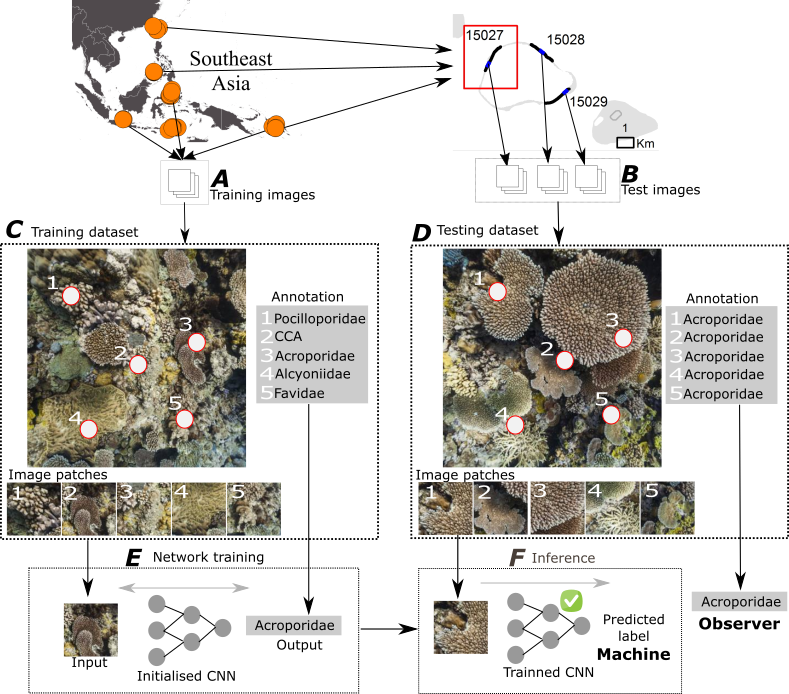
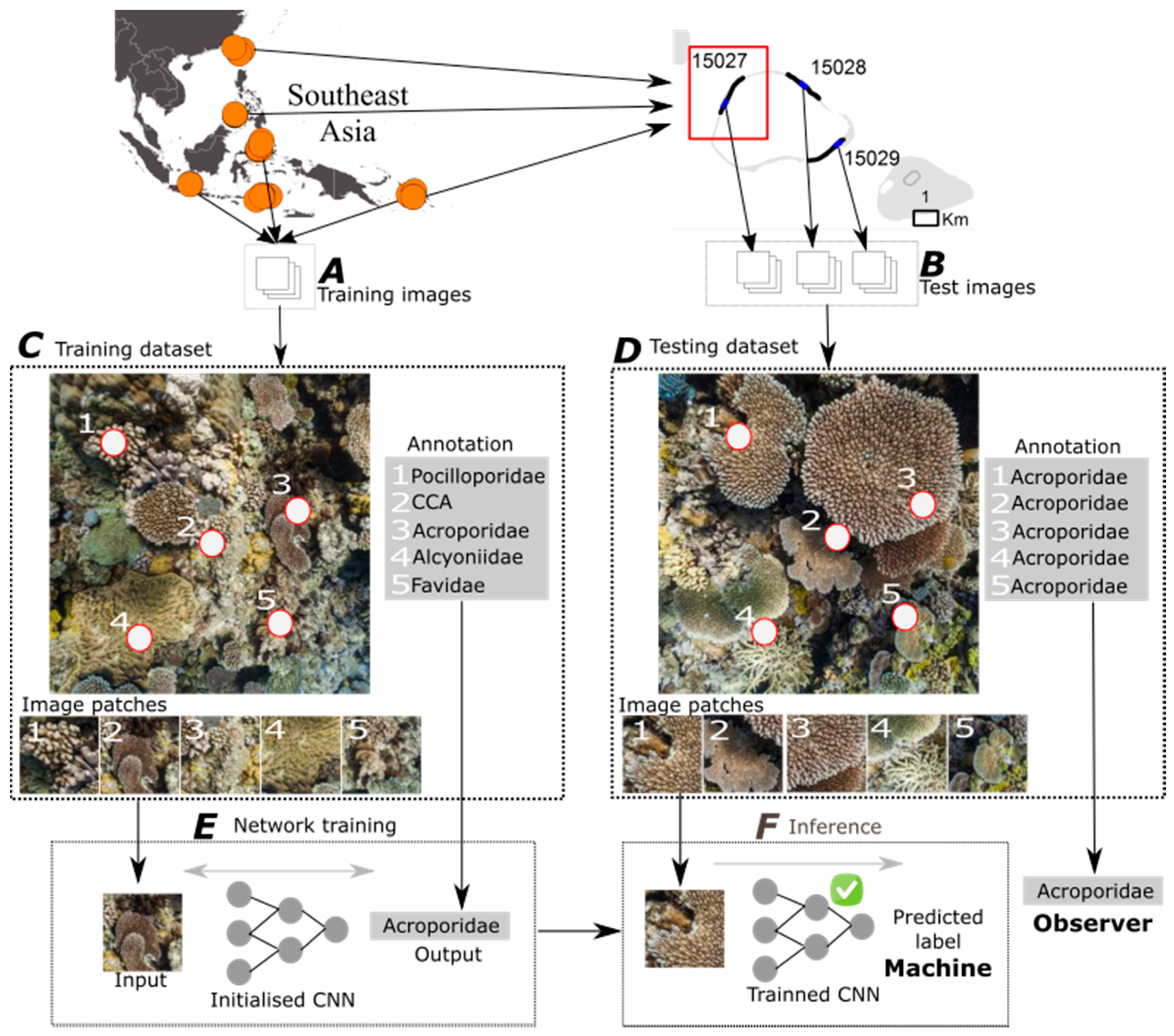
2.2.1. Overview

This study builds on a long line of work in Artificial Neural Networks (ANN) [12], in particular on the use ANN for supervised classification of underwater images of coral reef benthos. Artificial Neural Networks are computing systems for machine learning inspired by biological neural networks. Such systems learn to do tasks by considering examples where images are classified based on associations. Deep Learning is a learning algorithm part of the family of machine learning methods based on ANN, built on the assumption that observed data are generated by the interaction of layered factors that explain a pattern (e.g., an object in an image). In this study, we used Convolutional Neural Networks (CNN), a class of deep learning networks commonly applied to analyse visual imagery.
After passing through the CNN, an image becomes abstracted into features or factors that are organised in a hierarchical way, where higher level factors or more abstract concepts (e.g., an object or a landscape) are learned from lower level or more basic layers (e.g., circles, square edges). Based on this concept, the CNN architecture uses a cascade of many layers to extract and transform features from an image. Each successive layer uses the output from the previous layer as input that construct more complex features that start resembling objects in the higher-level layers. In this way, the Convolutional Neural Network, hereafter referred to as network, is organised by layers forming a hierarchy from low-level to high-level features.
As the network is trained with a set of manually classified images the signal propagates back and forward through the network and the importance of each feature is weighted (backpropagation), through a number of iterations until the network reaches a maximum accuracy (Figure S4). This way the network helps to disentangle the abstractions of an image and pick out which features are more useful for improving the performance of the automated classification. The interpretation of the network output is done in terms of probabilistic inference, where the network outputs a probability (i.e., posterior probabilities) that an image belongs to each of the proposed labels or classes and, the predicted label with the highest probability is chosen for the classification.
Here, we used VGG-D 16 [21], a convolutional neural network architecture pre-trained or initialised on a large dataset comprised by ten million images and one thousand classes, ImageNet [22] (please refer SM2 for more details). The network parameters were fine-tuned by training iterations with our training dataset (Table S1, Figure S5), where the final fully connected layer, containing the classification units, was replaced by the specific label-set of the data (Table 1 and Table S2).
A network was trained for each country within the regions, except for the region Western Atlantic Ocean and the countries The Philippines and Indonesia, where one network was trained for each group using data from each country (Table 1). This means that, to produce classifications on new images, an additional manual intervention is required to select a trained network selected from a specific region before producing the automated classification. The classifications from each network were aggregated per region to evaluate the overall performance of CNN classifiers in this work. Countries within each region shared the same label-set, while regions comprised a unique taxonomic composition (SM3, Table S2).

2.2.2. Classification of Random Point Annotations

The network architecture implemented here has been designed for image classification, i.e., assigning a class to the whole image or scene. Here, however, we are interested in learning to automate random point annotation, i.e., the assignment of one class to a particular location in an image. This method, also referred to as random point count, is commonly used in many population estimation applications using photographic records [23]. In random point annotations, the relative cover or abundance of each class is defined by the number of points classified as such relative to the total number of observed points on the image.
The random point count methodology was used to generate annotations for two independent datasets for each region or country (Figure 2). One dataset, the training dataset (Figure 2A,C), corresponds to randomly selected images from the country or region that define each network. This dataset comprised between 350 and 1224 images were 100 points were manually classified by experts to train each network model. The second dataset, the testing dataset (Figure 2B,C), is described in the section below, comprises images manually annotated to define the reference dataset used to evaluate the performance of automated annotations from each network. The testing dataset was selected as a separate set of images from the training dataset to ensure complete independence from the data used to train the network models.
To achieve automated random point annotation, we converted each image to a set of patches cropped out around each given point location (i.e., image patch). The patch area to crop around each point was set fix to 224 × 224 pixels to align with the pre-defined image input size of the VGG architecture [21]. During the training process, the training dataset was used to fine-tune the network parameters through backpropagation, resulted in a fully trained network model. Once training achieved, the performance of the network was evaluated against the test dataset, where only the cropped image patches were provided to the trained network to infer the labels for each image patch (Figure S6, detailed in SM2).
Training and deployment (i.e., inference) of networks were implemented in Python using the “caffe” deep learning framework (cafee.berkeleyvision.org). All computations were performed on AWS Cloud Computing P2 instances, GPU scalable virtual computers configured for high-performance computing (Amazon Web Services, Amazon Inc., USA).

2.3. Performance of Automated Image Annotation

2.3.1. Test Transects

We evaluated the performance of automated estimations of abundance on the set of images and manual annotations defined above as testing dataset. This dataset was a selection of contiguous images within transects with an extent of 30 m in length, concomitant with most coral reef monitoring programs e.g., [24,25,26] and best represents the spatial heterogeneity within a site [18]. Therefore, we aggregated the images from the 2 km transects within a standard transect length of 30 m, hereafter called “test transects” (SM4). Test transects were selected at random, within the 2 km transects, while ensuring that no test transect contained images used for training the networks. The benthic composition within these transects was averaged across images and contrasted between the two methods evaluated in this study: manual vs. automated annotation. A total of 5,747 images, within 517 test transects (Table 1), were annotated by the networks, hereafter called “machine”, and a trained human observer, hereafter called “observer”.
Considering the aim of this study in evaluating the use of machine learning for coral reef monitoring, images were grouped within transects for three main reasons: (1) consistency in the definition of sample unit for coral reef monitoring; (2) evaluating the ability of automated methods in detecting change over time; and (3) compatibility of observations with existing monitoring data to evaluate continuity in coral reef monitoring data. In terms of consistency, image-based monitoring defines a sample unit as an aggregation of images that represent the condition of benthic communities in a given location (e.g., transects or quadrats within a site). Therefore, the aggregation of images within transects allowed evaluating the performance of automated estimation within a scale that is consistent with monitoring sampling units, accounting for the variability in benthic abundance estimation among images. Because the aggregation of images within sampling units allows to capture the condition of a reef site or location in a given point in time, this aggregation made possible the evaluation of changes over time when considering sampling errors in the placement of such images within permanent or semi-permanent transects. Lastly, being consistent in terms of sampling units also allowed to contrast automated estimations with existing monitoring data from external programs to evaluate the long-term integrity of monitoring archives when implementing novel technologies for automation. Should a reader be interested in the metrics of performance described below at the image level, please refer to SM4 (Figure S7).

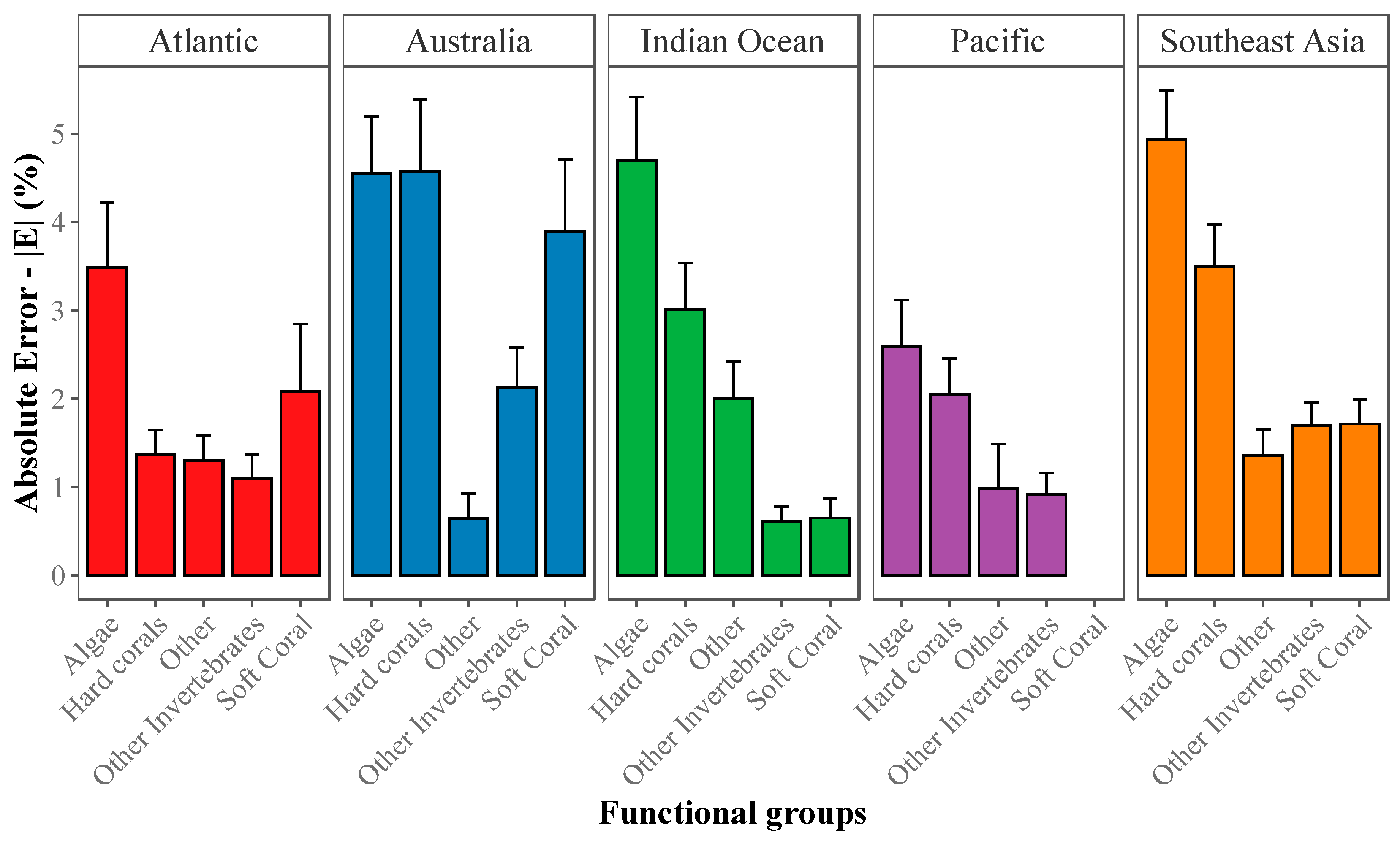
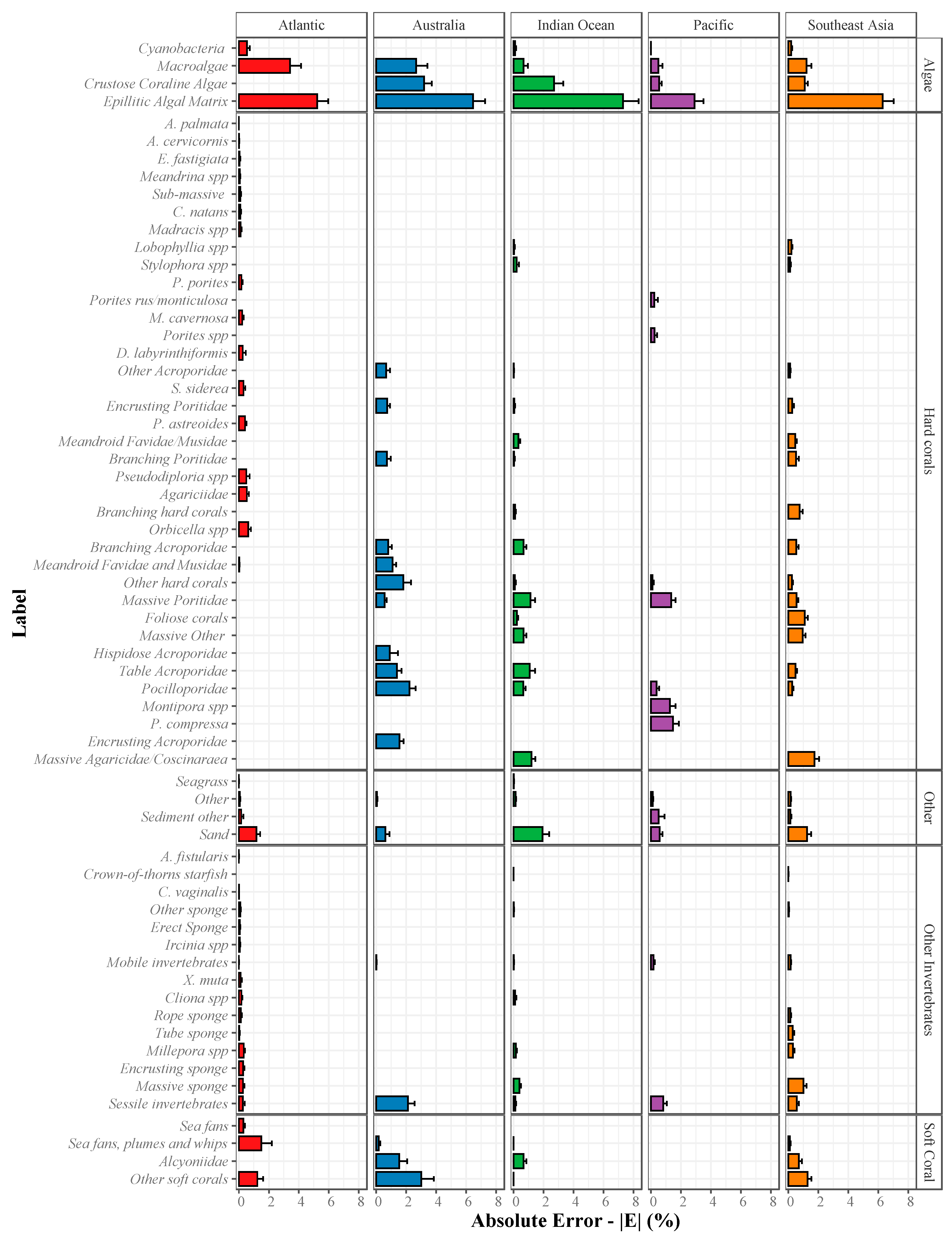
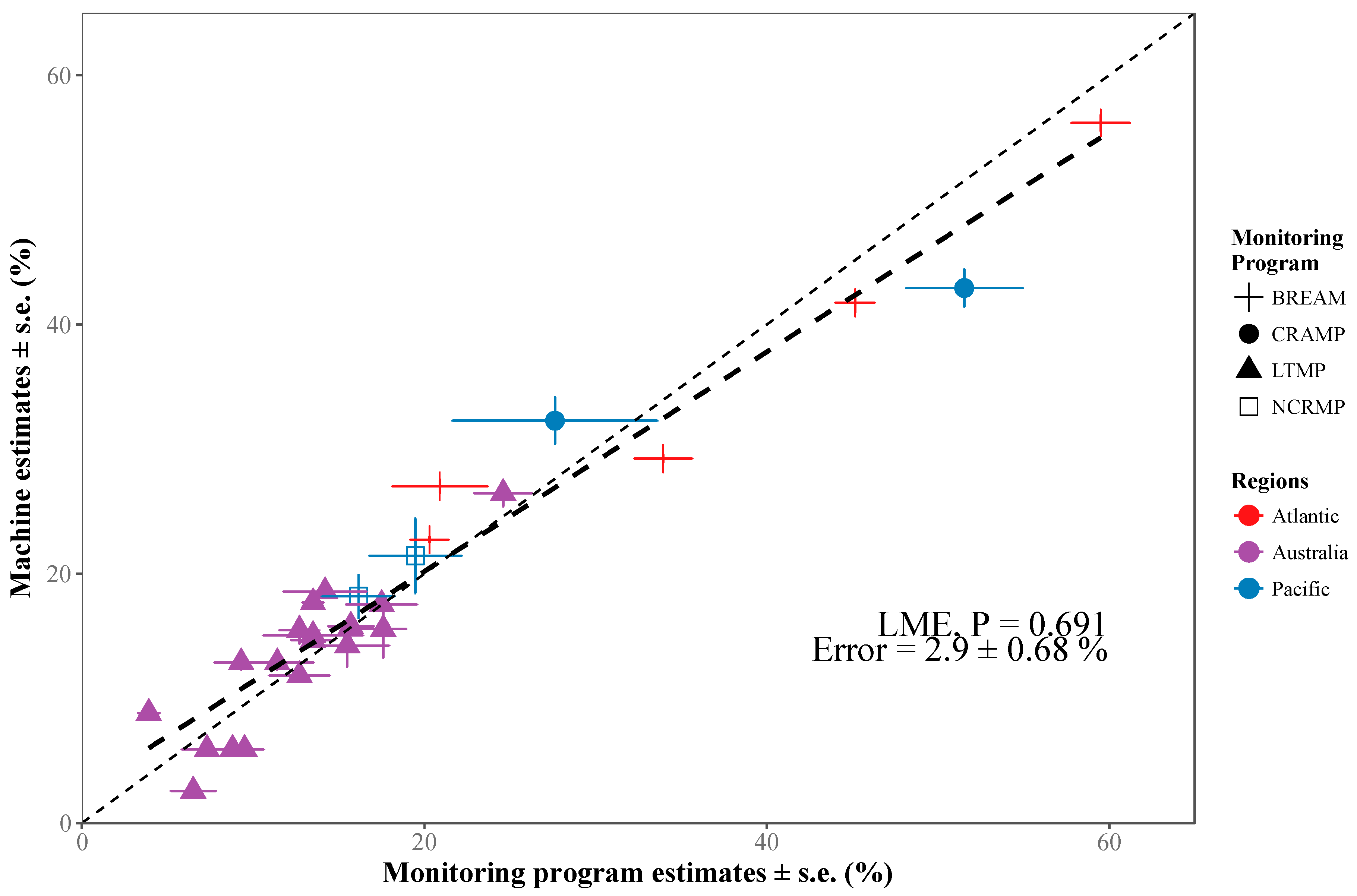
2.3.2. Absolute Error (|E|) for Estimation of Abundance

An error metric was used to represent the overall difference between machine and observer abundance estimations for each label. Machine estimations tend to be unbiased from observer estimations but rather noisy (i.e., mean of difference between machine and human tend to zero with a variance around the mean, Appendix A). Therefore, we evaluated the Absolute Error (|E|) to estimate the variability in the machine estimates when compared against observer estimations of abundance of a given label. The absolute error (hereafter name error) for each label (i) was calculated as the absolute difference between the abundance estimated by the machine (m) and the observer (o; Equation (1)). The error was calculated and compared at two aggregation levels: (a) major functional groups and (b) full label-set, sensu González-Rivero et. al. [18]:
| E | i = | m i o i |

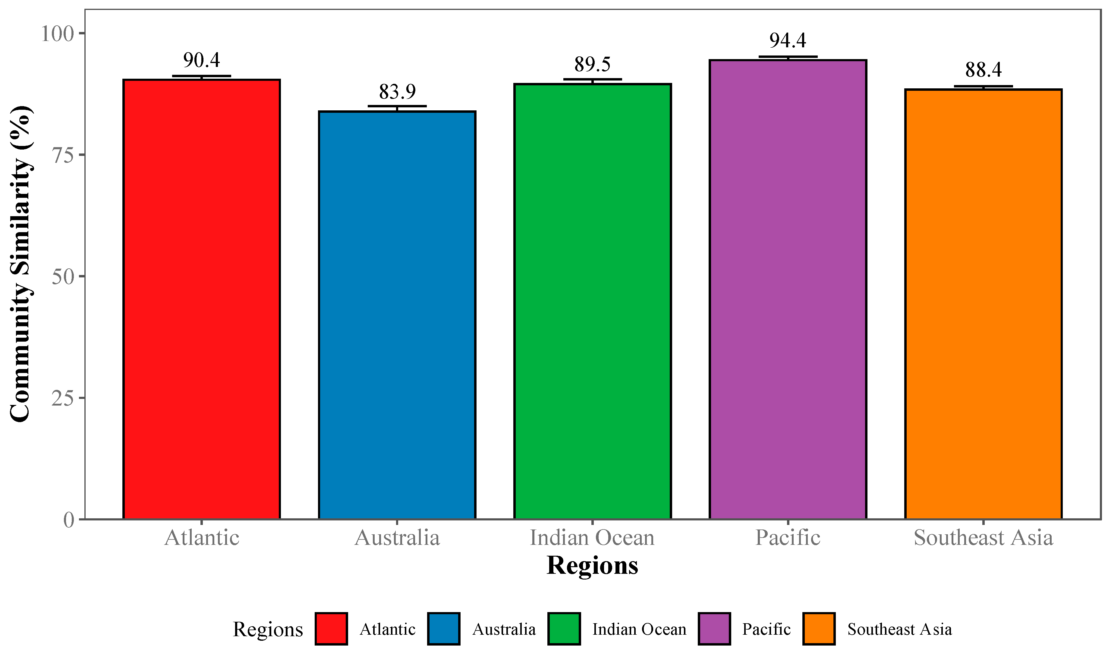
2.3.3. Community-Wide Performance

To evaluate the machine performance for estimating community composition, pair-wise comparisons of manual and automated estimations of benthic composition within each test transect were performed using the Bray-Curtis similarity index. This index is sensitive to misrepresentation in the automated estimation of abundance for specific labels or benthic groups when compared against manual observations. Therefore, index values of 100% will represent a complete resemblance between machine and observer estimations for community composition. While the Absolute Error already provides a metric for label-specific performance of automated annotations, the community-wide analysis lay out a synthesis analysis to understand how closely represented is the automated estimation of benthic composition against manual observations across the range of community assemblages within a region.

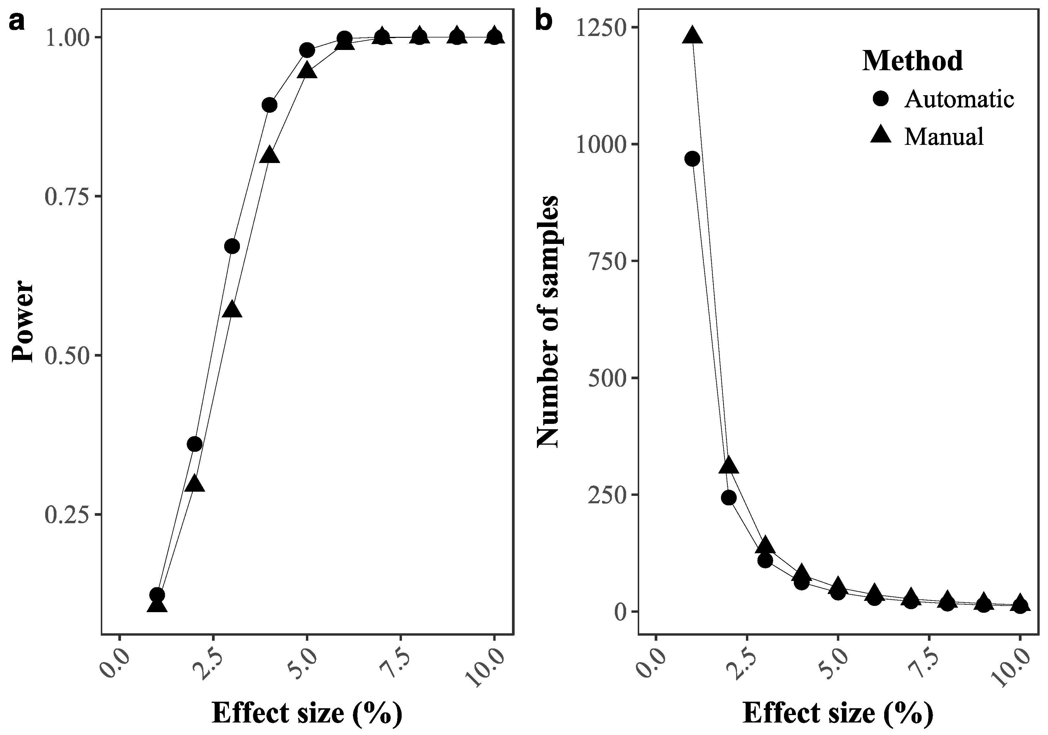
2.3.4. Ability to Detect Temporal Changes in Coral Cover

The consistency of the error over time can influence the capacity of machine-based monitoring to replicate the detectability of temporal trends by expert observations. The introduced variability may hinder the detectability of small changes (using similar size), limiting the applications of machine-based monitoring. A power analysis was used to evaluate whether machine-based analyses can replicate the detectability of change in coral cover from expert observations (power) across a gradient of coral cover changes over time (size effect).
For transects surveyed in multiple years in Australia, Central Indian Ocean and Central Pacific Ocean, the absolute change in coral cover was compared between observer and machine estimations. Power was calculated in R (v3.4.0) using a paired t-test function (power.t.test) to account for repeated surveys within transects [27].

2.3.5. Data Continuity in Coral Reef Monitoring

Long-term continuity in monitoring is essential to identify baseline patterns, detect early warning signals and ensure robust forecasting of the ecosystem trajectories [2]. Novel technologies, therefore, need to preserve the long-term integrity of monitoring archives [28]. To evaluate this, we contrasted automated estimations of coral cover (XL-CSS data) against manual estimations from different monitoring programs using a linear mixed-effect regression (LME). In this regression, pairwise average estimations of coral cover per site were compared between methods (fixed effect), accounting for each site within monitoring programs (random effect).
Four programs, in three of the surveyed regions, coincided with XL-CSS survey sites: Bermuda Reef Ecosystem Analysis and Monitoring (BREAM, Bermuda Zoological Society, Atlantic; [25]), Long Term Monitoring Program (LMTP, Australian Institute of Marine Science, Australia; [26]), Coral Reef Assessment and Monitoring Program (CRAMP, Hawai’i Institute of Marine Biology, Pacific; [24]), and National Coral Reef Monitoring Program (NCRMP, National Oceanographic and Atmospheric Administration, Pacific; [29]). These programs commonly use photography and manual point-count scoring of these images to extract the coverage of benthic groups. Monitoring sites were selected based on the proximity to the XL-CSS sites (within a radius of two km, SM5 and Table S3).

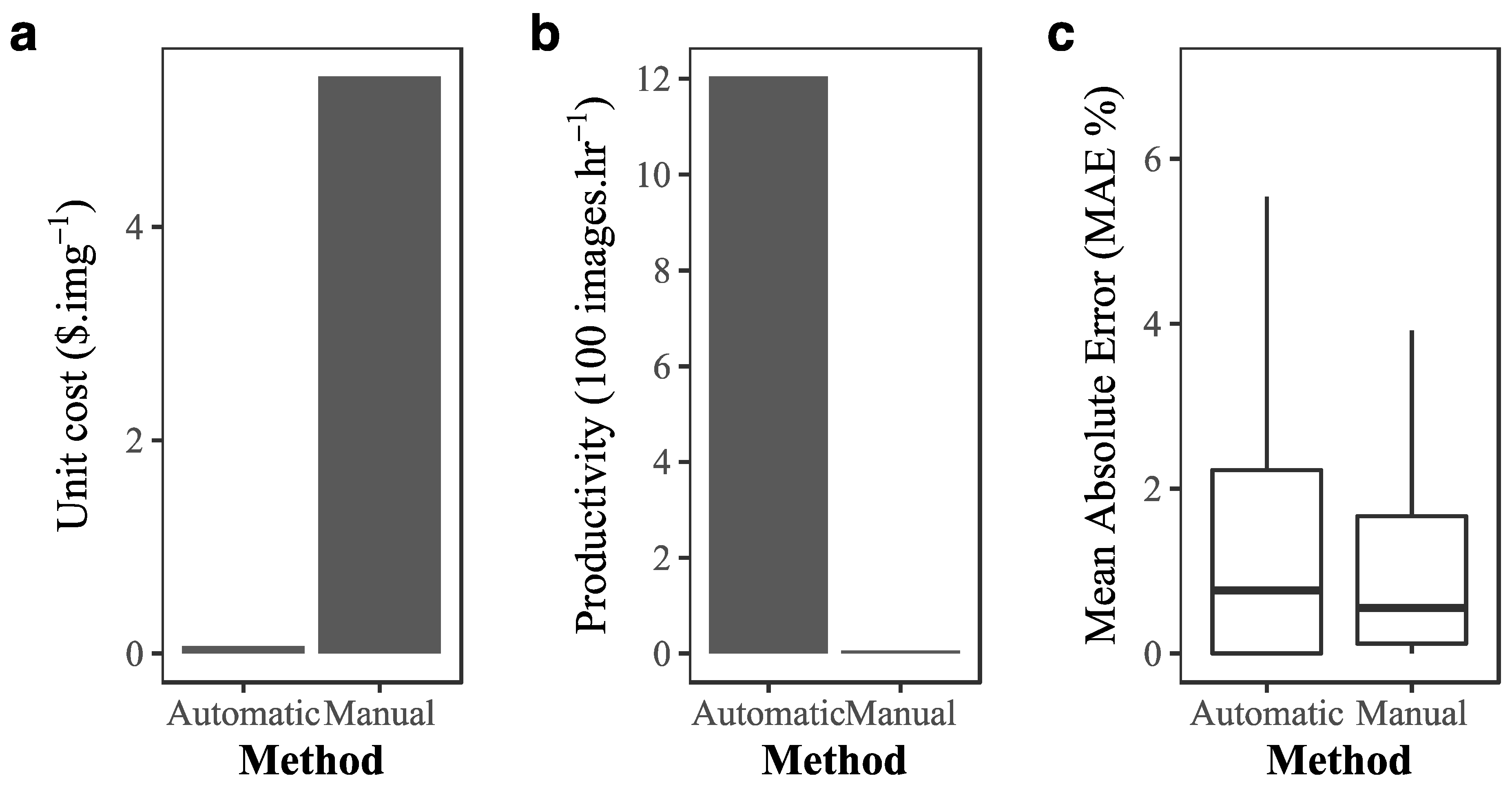
2.4. Cost-Benefit of Implementing Deep Learning in Coral Reef Monitoring

Our final question assessed the viability of automated analysis in existing coral reef monitoring program. In an attempt to address this question, we performed a cost-benefit analysis circumscribed to the image analysis, based on our experience. Cost, efficiency and performance of automatically and manually annotated images were contrasted. In terms of costs, we calculated the unit value of processing an image by an expert observer compared to the estimated cost of automated image processing using the cloud computing services (Amazon Inc.). We used the casual hour rates for an experienced biologist at the University of Queensland (US $33.83/hr, HWE 5, https://staff.uq.edu.au/information-and-services/human-resources/pay-leave-entitlements/pay-scales/professional-research) as well as the efficiency of this expert annotator (images.hr-1) to estimate the cost of manually annotating a single image. In the case of machine learning, this calculation was comprised of two main components: the cost of cloud computing time and the cost of manually annotating images for training and testing the network. Also, an additional ongoing cost is considered in the form of the expert labour and computational time required every time a new set of images needs to be processed. In terms of efficiency, we contrasted the productivity of annotation (images.hr-1), manually and automatically (SM6).
The performance of automated image annotation was calculated as described above. The range of errors observed across the label-set was against the interval of errors for multiple observers (inter-observer variability), previously estimated using the same label-set and images from the Australia region [18].

3. Results

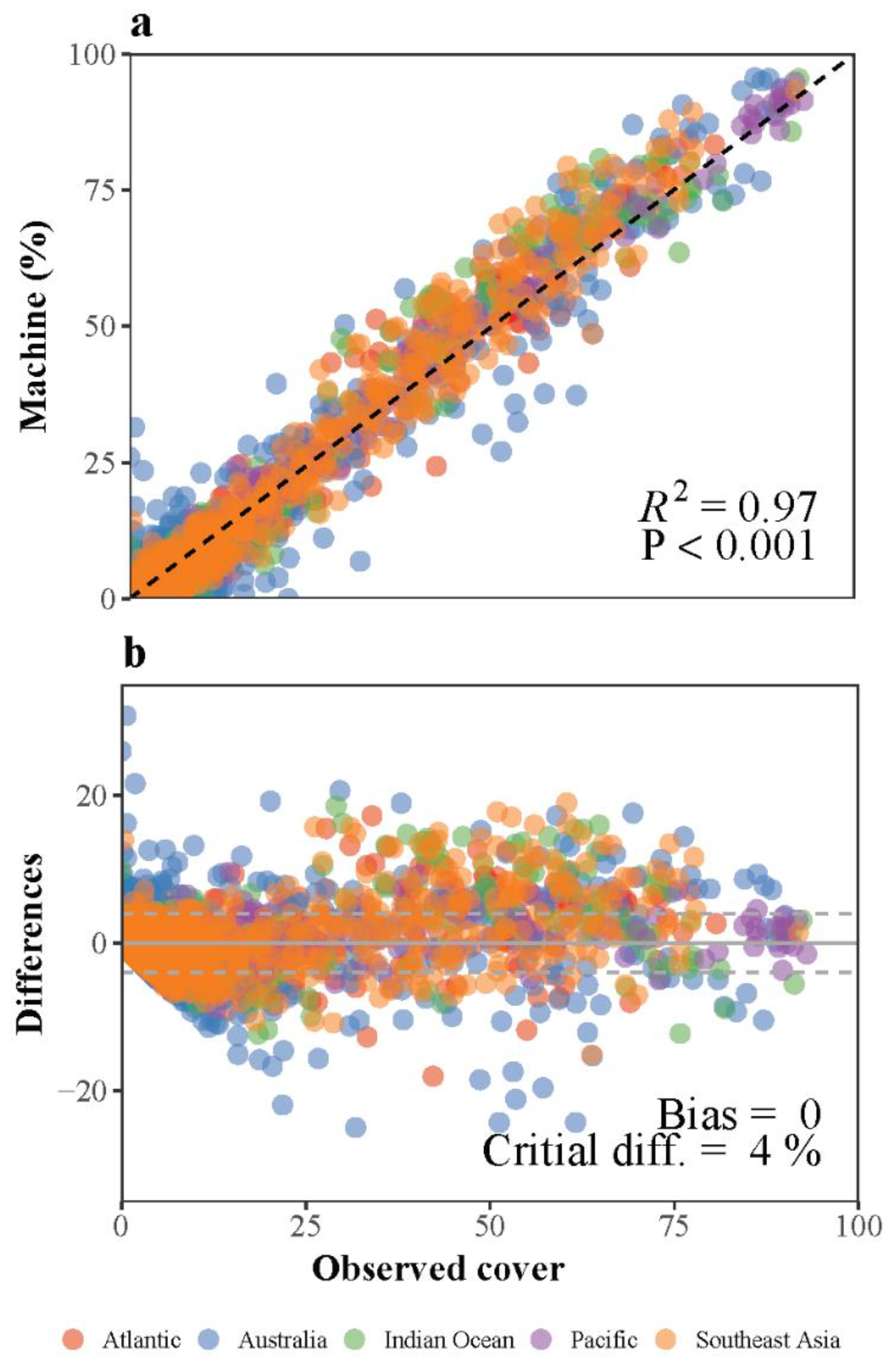
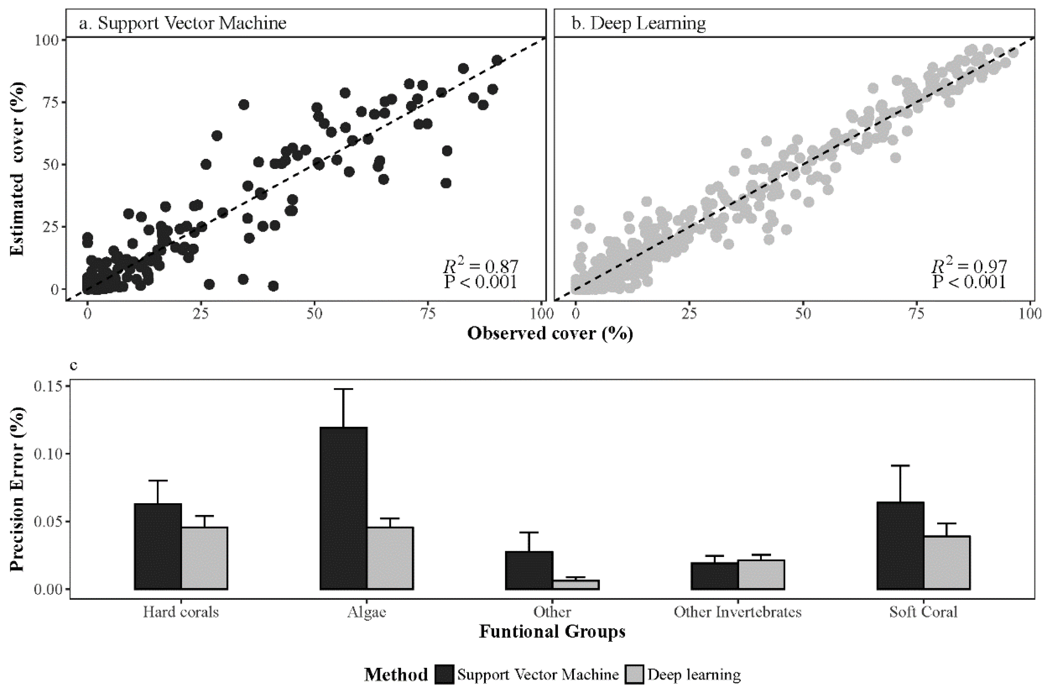
3.1. Deep Learning Performance

Network estimations of benthic coverage were highly correlated with observer estimations for all five global regions (R2 =0.97, P < 0.001, Figure A1), better than shallow learners (SVM, Figure A2). The differences between the machine and observer were unbiased across the spectrum of benthic coverage (mean ~ 0), and the variability around the mean difference was estimated at 4% (Critical Difference or 95% Confidence Interval of the difference) for all labels across the study regions (Figure 3, Figure 4 and Figure A1).
Among major functional groups (e.g., hard corals, algae), the error in abundance estimations varied most notably among classes and less so among study regions (Figure 3). Algae was the most variable class (3%–5% error). Hard and soft corals were the second most variable group in terms of error. The abundance of hard corals estimated by the machine showed a higher agreement in the Atlantic and Pacific Ocean regions, where the error ranged between 1% and 2%. For the other regions, the error for hard corals ranged between 3% and 5%. Other classes showed a consistent error below 2% (Figure 3).
Within major groups (i.e., higher taxonomical resolution), the error of machine estimates was more consistent, with the only exception of classes within the Algae group (Figure 4). Epilithic Algal Matrix (EAM), as a functional group, comprised by a diverse number of algae groups (e.g., macroalgae, cyanobacteria) was the most variable label (5%–7% error). The error of estimations, within the hard-coral groups, remained below 2% among regions, while soft corals, in particular “Other Soft corals” showed an error of up to 3%. This label is comprised by a large diversity of genera and growth forms, while more taxonomically defined labels showed an error below 2%. The remaining classes within the groups of “Other”, comprised mainly by substrate categories (e.g., sand, terrigenous sediment), and “Other Invertebrates”, comprise of benthic invertebrates other than hard and soft corals, showed a consistently low error (below 1%–2%; Figure 4).
Across community assemblages within regions, the estimations of benthic composition were between 84% and 94% similar to observer estimations across regions, irrespective of the differences in community structure among and within regions (Figure 5). Across regions, Australia exhibited the lowest values of similarities, 84%, while automated estimations of benthic composition from the Central Pacific Ocean shared 94% similarity with manual observations.
The analysis of the power of detection for temporal trends showed that both machine and observer estimations of change in coral cover were very similar across a gradient of change in coral cover (effect size; Figure 6a), both reaching a power above 0.8 when the effect size (i.e., absolute change in coral cover) was above 4%. Similarly, the number of samples required to achieve a power of 0.8 was the same for either machine or observer estimations across the effect size (Figure 6b).
Automated coral cover estimates from our survey imagery (XL-CSS) were contrasted against reported values from different monitoring programs, to evaluate data continuity in long-term monitoring. Pair-wise comparison in coral cover estimations by automated image analyses and those by each monitoring surveys shows an overall agreement across regions and an average error of 2.9%, in line with the errors reported above (LME, P = 0.691, error = 2.9%, Figure 7).

3.2. Cost–Benefit Analysis of Implementing Deep Learning

The cost of annotating a single image by an expert was estimated at US$ 5.41, while using machine learning was only US$ 0.07 (1.3% of the cost for manual image annotation, Figure 8a,b). Furthermore, the error of network estimations was comparable to the error associated with multiple observers. However, a slightly higher variance of the error was observed in the machine estimations compare to the inter-observer error (Figure 8c). In terms of productivity, networks can annotate 1200 images per hour, while manually this would require 16 h of continuous work. This rate of productivity is equivalent to a 200-fold increase compared to traditional manual image annotation.
It is important to highlight that ongoing costs for this automated framework should also be considered to cover the expert labour and computational time required every time a new set of images is to be processed. Depending on whether this new image set requires a new architecture, training and calibration for the CNN network, or just the implementation of a pre-trained and calibrated network, these costs are estimated to range between US$600 and $1740 for every 50k images, based on our experience (see SM6 for more details).

4. Discussion

Automated estimations of benthic coverage were in agreement with those manually generated by expert observers for all five global regions. Similarly, Williams et al. [30] found high consistency between the cover estimations done by machine and observers using images from Hawaii and American Samoa and CoralNet, which is an online platform designed for automated image analysis based on deep learning (www.coralnet.ucsd.edu). The use of deep learning was also superior in performance when compared to shallow learning approaches (i.e., Support Vector Machine, SVM). With low errors, comparable power in detecting temporal trends to expert observations and a productivity that is at least 200x higher than manual labour, at fractional cost of manual data extraction (1%), the results of the present study make a very strong case for implementing deep learning in coral reef monitoring. It is important to add a couple of caveats. Firstly, there are limitations in terms of the taxonomic resolution, which may or may not be important depending on the question being asked. The ability of machines to detect objects is, however, likely to improve over time as machine learning innovations continue to escalate. Secondly, while monitoring of coral reefs can benefit from fast processing and data standardisation powered by automated image analyses, an integration between human expert observations and machine learning may be recommended in some circumstances.
According to our results, the errors introduced by implementing deep learning in automated abundance estimations (2%–6%) are within the range of previously reported inter- and intra-observer variability for established monitoring programs (e.g., 2%–5%, Long Term Monitoring Program, AIMS, Australia; [8]), where the variability introduced by automated estimations of abundance are well below the range of spatial and temporal changes observed in nature [8,9,31]. Concomitantly, the introduced error by automated annotations had little influence over the detection of change in coral cover, because the statistical power for detecting significant change resulted virtually identical between expert and automated estimations. Furthermore, data continuity was not constrained by implementing automated image processing given that these estimations are highly compatible with established monitoring programs, which ensures consistency in long-term monitoring [2]. Therefore, we conclude that errors introduced by networks are unlikely to limit the effectiveness of machine-based systems in monitoring change.

4.1. Challenges and Further Considerations in Automated Benthic Assessment

Challenges posed by the visual identification of species from imagery, taxonomic/functional definition of labels, inter-observer variability in abundance estimations and innate aspects of automated image annotation can partially explain observed errors.
As one label typically contains several morphologically diverse taxa, the taxonomical complexity or potential number of species within a label can introduce variability in the accuracy of automated classifications. The definition of labels influences the error of automated classifiers, in terms of innate capacity of the machine to identify each label, as well as the error introduced by inter-observer variability in the training of network models. A key example is the algae group, comprised of a large number of species, with an estimate of 630 for the Great Barrier Reef alone [32], and are only represented here by five functional groups or labels (Epilithic Algal Matrix, Macroalgae, Crustose Coralline Algae and Cyanobacteria). Therefore, variations in the visual attributes that define each species within a label adds confusion in terms of identification [17,30]; also observed here. Arguably, inter- and intra-observer variability drives larger errors per class because the training and test datasets derive from variable observer estimations [8,17,18]. While separating both effects (machine-introduced and inter-observer error) can be difficult, more defined labels will yield to lower errors in automated analyses [17]. This can be observed when comparing the overall error and community-wide agreement among regions, where more defined label-sets and lower taxonomic complexity (e.g., Eastern Atlantic and Central Pacific, Table 1), showed the lowest error and highest community similarity between manual and machine observations. Arguably, a relationship between mean observed values and the variance of automated annotations could explain that aggregated labels (e.g., Hard Corals) will be more abundant than taxonomically defined labels (e.g., Montastraea cavernosa) and therefore present larger errors. However, an analysis of the error of automated estimations across the mean of observed values shows no bias or over dispersion of the error (Figure A1). However, the aggregation of labels into larger benthic categories may carry forward sources of error in machine annotations that lead to slightly larger discrepancies between machine and observer estimations.
Visual traits of coral reef benthos can also pose several challenges for estimations of abundance. Among these traits, there are: (1) plasticity of forms, (2) visual similarity among phylogenetically distinctive organisms (e.g., algae and corals, soft-corals and hard-corals), (3) undefined shapes and edges (e.g., algae), (4) intricate growth among organisms (e.g., algal matrices), and (5) different magnification scale required to accurately identify organisms.
Environmental regimes (e.g., wave action and light) can heavily influence the morphology of sessile organisms [33]. A single taxonomical classification can be visually distinct in response to environmental regimes, thus introducing variability in the training data. For example, hard coral species from the genera Orbicella and Siderastrea, typically from massive mound or branching morphologies, but in light deficient environments (e.g., at depth), the same species will adopt plating morphologies, maximising their capacity to capture light [34]. Considering morphological traits in the classification scheme may allow to account for phenotypical plasticity among environmental regimes, maximising the consistency of the training dataset, hence the machine performance.
Ill-defined edges, patchiness, intricate growth and the different resolution of taxonomic attributes in marine benthos can also add complexity in their identification using point-based abundance estimations. A clear example is the classification of algae, which consistently showed the highest error (3%–6%) across regions, concurring with other studies [17,18,30]. If the definition of the algae is too patchy (e.g., turf algae) or it is growing among other algae species (e.g., macroalgae), higher magnification maybe needed to resolve its taxonomy. The approach used here for automated image identification defines a fixed window size, on which the machine extracts and weights the importance of visual attributes (e.g., texture, colours) to assign a label. Well-defined and large organisms, such as corals and soft corals, showed the lowest error (1%–2%) when observed in our window size. This window size, however, penalises the estimation of smaller, patchy or less defined organisms, such as Epilithic Algal Matrix (EAM, error ~ 3%–6%). Using multi-scale or regional networks to account for the taxa-specific model sensitivity (e.g., [35]) may help by increasing versatility in the definition of the region of interests and maximising the accuracy of abundance estimations. Furthermore, light spectral signature (e.g., fluorescence, reflection) may offer an alternative to expand the parameters that define phototrophic or pigmented organisms [36,37].
Machine learning is a constantly evolving field and a diversity of alternative classifiers and software frameworks are available. While the VGG architecture, used in this study, remains in the top tier of image classifiers in terms of classification errors [38], newer and deeper convolutional neural network models are less computationally intense (faster) architectures, slightly improving in classification error benchmarks [39]. Similarly, newer software frameworks (e.g., Tensorflow, Keras) are now faster and easier to implement than Caffe, offering greater versatility in its applications [40]. Further work to compare the network architecture and software framework will provide a better overview for choosing the best configuration that fits the purpose of individual applications of this technology.
Looking forward, this work comprises a specific network model for each country/region (Table 1) and a more advanced system, accounting for the geographic origin of the data, will facilitate its applications in global monitoring. Furthermore, propagating the classification uncertainty from the machine into statistical analyses will ensure a more robust integration and interpretation of monitoring data (e.g., [41]).

4.2. Implications of Automated Benthic Assessments for Coral Reef Monitoring

It is important to understand the cost-effectiveness of machine-based monitoring relative to more conventional methodologies. Here, we demonstrated several breakthrough steps with machine-based monitoring. These include scale, repeatability, rigour, speed of reporting, and cost-effectiveness. While it is argued here that automated image analysis is not to replace expert observations in monitoring, the higher efficiency (200×) and lower costs (1.3%, plus reduced ongoing costs) provide compelling reasons for being adopted over conventional human-based techniques. This advantage becomes clearer when one considers the large volume of images [18], increasing demand for reporting (e.g., [42]) and large management extents [1]. Automated image annotation offers the possibility of alleviating back-logs and accelerating the availability of detailed and accurate monitoring data, allowing relocating limited resources (e.g., expert staff) towards detailed and needed observer-derived data (e.g., biodiversity assessments). In this way, automated assessments can provide an avenue to expand the detail in monitoring by reallocation of resources, while significantly reducing the reporting time for large scale metrics (e.g., changes in composition).
Machine-based monitoring has the advantage of data integration, where once an image is collected, it can be revisited and automatically processed over time. Data integration often generates invaluable insights on the status and trends of ecosystems at global and regional scales [43,44]. Nonetheless, much more could be done to harness the vast amounts of data collected by government agencies, NGOs, citizens and scientists [6]. As a common monitoring tool, images generate valuable and standardised information, which paired with automated image analyses can ease data integration, without impairing long-term data continuity. The number of open-access online tools for automated image annotation and robust demonstrations of their applications across conservation disciplines [16,30,45,46] is rapidly increasing. Critical steps are now needed to capitalise on these efforts [28,47] and maximise the advantages of a global monitoring and conservation science empowered by machine learning.

5. Conclusions

Automated image recognition via Convolutional Neural Networks introduced an improved image classification, compared to more classic machine learning approaches, with an unbiased agreement between expert and automated observations of 97% and an overall error of 4%. Community composition indices revealed that this agreement is also maintained at community levels (83%–94% across bioregions). The error varied across taxonomic groups and indicate that a functional taxonomic resolution, attainable by trained observers, is also possible by using automatic methods. The application of artificial intelligence in automated image classification can reduce significantly the bottleneck in data processing and reporting of coral reef monitoring by accelerating image analysis at least 200x, at a fraction of the cost estimated for manual image annotation (1%).

Supplementary Materials

The following are available online at https://www.mdpi.com/2072-4292/12/3/489/s1, Figure S1: Post-processing of images for automated classification, Figure S2: Comparison between post-processing methods of precision errors of automated image annotation for each label within the Maldives, Central Indian Ocean, Figure S3: Comparison between post-processing methods of precision errors of automated image annotation for each of label within the Great Barrier Reef, Figure S4: Fine-tuning of networks, Figure S5: Absolute Error for the abundance estimation of benthic classes (Labels) by different net configurations, Figure S6. Diagram to visualise the approach to automatically estimate the relative abundance of benthic groups using a sample image, Figure S7. Absolute error (|E|) for automated estimation of benthic abundance within an image, Table S1: Configuration parameters for each network after fin-tuning weights and calibrating the learning rate and receptive field, Table S2: Label set defined for automatically identifying coral reef benthos per region, Table S3: Summary of locations from monitoring programs in Hawaii, Bermuda and Australia used to compare the capacity of automated image analysis to ensure data continuity.

Author Contributions

M.G.-R., O.B. and A.R.-R. conceived the ideas and designed methodology; M.G.-R., A.R.-R., A.G., D.E.P.B., A.T., K.S., E.M.S., C.J.S.K., E.V.K., B.P.N., C.R.-N., J.V., K.M., Y.G.-M., and A.H.-R. collected the data; M.G.-R., A.R.-R. and S.L.-M. analysed the data; M.G.-R. led the study and writing of the manuscript. All authors, including K.O., M.W. and O.H.-G., contributed critically to the drafts and gave final approval for publication. All authors have read and agreed to the published version of the manuscript.

Funding

This research was funded by XL Catlin Ltd. (now AXA XL; to OHG and MGR) and the Australian Research Council (ARC Laureate and ARC Centre for Excellence to OHG). The production of this work was also funded by Vulcan Inc (OHG), including the article processing charges (APC).

Acknowledgments

The authors are grateful to: the XL-CSS, the Global Change Institute, the Ocean Agency, Underwater Earth, Selene Gutierrez, Morana Mihaljevic, Angela Marulanda, Veronica Radice, Christophe Bailhache, the Waitt Foundation, the Living Oceans Foundation, the Joy Family Foundation, the Australian Department for Energy and Environment, CARMABI, BIOS, the Indonesian Institute of Science, NOAA and IUCN for their support. MGR thanks Hugh Sweatman, Greg Coleman, Thad Murdoch and NOAA for kindly providing data to construct Figure 7 and, Janice Lough for her comments on earlier versions of the manuscript.

Conflicts of Interest

All authors declare no conflict of interest.

Data and Code Source

Images and annotations are accessible through the following data archive: https://espace.library.uq.edu.au/view/UQ:734799. The documented code and examples to implement the automated image analyses method from this study can be found in the following repository: https://github.com/mgonzalezrivero/reef_learning.

Appendix A

Overall Performance of Deep Learning Convolution Neural Networks

The overall performance of automated image annotation was evaluated by (1) correlating the estimates of abundance (i.e., cover) produced by the machine against those produced by the observer and (2) evaluating the overall agreement between machine and observer estimations using the Bland-Altman plots, also called difference plots. Correlation was evaluated using the coefficient of determination from a linear regression model, which also evaluated the significance of this correlation. The coefficient of determination (R2) provides an indication of the intensity of the correlation by the evaluating the co-variance between the observer and machine estimations. The Bland-Altman plot determines differences between the two estimations against the observer estimations, or reference sensu [48], used to evaluate: (1) the mean of the difference or bias of machine estimations, (2) the homogeneity of the difference between techniques across the mean (over-dispersion) and, (3) the critical difference or agreement limits. The latter refers to the range, within the 95% confidence interval, of the difference between the two methods, and can be used as a reference to define where the measurements fall out of the range of the agreement (precision of the agreement). Bias refers to the difference between the two methods and the Bland-Altman plot can help visualising whether this bias change across the mean of values evaluated, and therefore a measurement of the consistency of the bias [49].
Figure A1. Overall agreement between network (machine) and manual (observer) estimation of abundance (cover). Agreement is here discretised in two metrics: (a) Correlation between machine and observer annotations and (b) bias. Each filled circle in these panels represents the estimated cover for a single by the machine and the observer in a given transect. The correlation shows that estimations of benthic abundance by expert observations are significantly represented by the automated estimations (R2 = 0.97). The Bland-Altman plot shows that overall the differences (Bias) between machine and observer tend to mean of zero (grey continuous line), and a homogenous error around the mean, defined by Critical Difference (Critical Diff.) or the 95% confidence interval of the difference between observers and machines (dashed grey lines).
Remotesensing 12 00489 g0a1
When compared to a shallow learning approach, Support Vector Machine [18], deep learning CNN was better at being able to resolve a wide range of benthic classes from the images (Figure A2). While the correlation between benthic cover estimates from both methods compares closely to the estimates obtained by observers (Figure A2a,b), the estimations from SVM are noisier compared to deep learning CNN (R2 = 0.87 vs. R2 = 0.97; Figure A2), thus, a significantly lower precision errors (Linear regression, P < 0.001) was detected among most functional groups using networks, with the only exception of “Other invertebrates” (Figure A2c, refer Table S2 for a description of this label).
Figure A2. Comparison of abundance automatically estimated by Deep Learning CNN and Support Vector Machines against manual annotations. The correlations between automated image annotation and manual annotations for all labels show the overall performance of both methods: Support Vector Machine (a) and Deep Learning CNN (b). Precision errors (or Absolute Errors) estimated within major functional groups show a more detailed comparison between the two techniques, where estimations of abundance by Support Vector Machine are more variable than those from Deep Learning CNN (c). Bars represent the average precision error and error bars show the 95%- Confidence Intervals for each functional group.
Remotesensing 12 00489 g0a2
Typically, given a set of training examples, each marked as belonging to one or the other categories, an SVM training algorithm builds a model that assigns new examples to one category or the others, making it a non-probabilistic linear classifier. An SVM model is a representation of the examples as points in space, mapped so that the examples of the separate categories are divided by a clear gap that is as wide as possible. New examples are then mapped into that same space and predicted to belong to a category based on which side of the gap they fall.
A Support Vector Machine solves an unconstrained optimization problem by maximising a loss function defined by the weight vector of classifications for each label. The effectiveness of SVM depends on the selection of kernel, the kernel’s parameters, and soft margin parameter (C). In the SVM study, the authors used Gaussian kernel, which has a single parameter (Gamma). The best combination of C and Gamma was optimised in grid search with exponentially growing sequences of C and Gamma, contrasted against the loss function for a total of 40K iterations (sensu the approach described here for Deep Leaning, Figure S4). Following this approach, the SVM model compared here against the deep learning network was trained using a subset of same imagery annotations from this work Eastern Australia, year 2012, following the approached described by Beijbom et al. [17] and the results validated in Gonzalez-Rivero et al. [18].
It is important to note that machine learning is a constantly evolving field and a diversity of alternative classifiers and software frameworks are available. The comparison between VGG and SVM presented here only add to the evidence that deep learning CNN has a superior performance than other shallow classifiers. While VGG remains in the top tier of image classifiers in terms of classification errors, newer and deeper convolutional neural network models now offer less computationally intense (faster) architectures, slightly improving in classification error benchmarks. Further work to compare different deep learning CNN architectures for ecological classifications are advised to provide better overview that help choosing the best machine learning configuration that fits the purpose of individual applications in ecology.

References

  1. Yoccoz, N.G.; Nichols, J.D.; Boulinier, T. Monitoring of biological diversity in space and time. Trends Ecol. Evol. 2001, 16, 446–453. [Google Scholar] [CrossRef]
  2. Lindenmayer, D.B.; Likens, G.E. The science and application of ecological monitoring. Biol. Conserv. 2010, 143, 1317–1328. [Google Scholar] [CrossRef]
  3. Nichols, J.D.; Williams, B.K. Monitoring for conservation. Trends Ecol. Evol. 2006, 21, 668–673. [Google Scholar] [CrossRef] [PubMed]
  4. McCook, L.J.; Ayling, T.; Cappo, M.; Choat, J.H.; Evans, R.D.; De Freitas, D.M.; Heupel, M.; Hughes, T.P.; Jones, G.P.; Mapstone, B. Adaptive management of the Great Barrier Reef: A globally significant demonstration of the benefits of networks of marine reserves. Proc. Natl. Acad. Sci. USA 2010, 107, 18278–18285. [Google Scholar] [CrossRef] [Green Version]
  5. Mills, M.; Pressey, R.L.; Weeks, R.; Foale, S.; Ban, N.C. A mismatch of scales: Challenges in planning for implementation of marine protected areas in the Coral Triangle. Conserv. Lett. 2010, 3, 291–303. [Google Scholar] [CrossRef]
  6. Hughes, T.P.; Graham, N.A.; Jackson, J.B.; Mumby, P.J.; Steneck, R.S. Rising to the challenge of sustaining coral reef resilience. Trends Ecol. Evol. 2010, 25, 633–642. [Google Scholar] [CrossRef]
  7. Aronson, R.B.; Edmunds, P.; Precht, W.; Swanson, D.; Levitan, D. Large-scale, long-term monitoring of Caribbean coral reefs: Simple, quick, inexpensive techniques. Atoll Res. Bull. 1994, 421, 1–19. [Google Scholar] [CrossRef]
  8. Ninio, R.; Delean, J.; Osborne, K.; Sweatman, H. Estimating cover of benthic organisms from underwater video images: Variability associated with multiple observers. Mar. Ecol.-Prog. Ser. 2003, 265, 107–116. [Google Scholar] [CrossRef] [Green Version]
  9. Ninio, R.; Meekan, M. Spatial patterns in benthic communities and the dynamics of a mosaic ecosystem on the Great Barrier Reef, Australia. Coral Reefs 2002, 21, 95–104. [Google Scholar] [CrossRef]
  10. Russell, S.J.; Norvig, P. Artificial Intelligence: A Modern Approach, 3rd ed.; Prentice Hall: Upper Saddle River, NJ, USA, 2009. [Google Scholar]
  11. Samuel, A.L. Some Studies in Machine Learning Using the Game of Checkers. IBM J. Res. Dev. 1959, 3, 210–229. [Google Scholar] [CrossRef]
  12. LeCun, Y.; Bengio, Y.; Hinton, G. Deep learning. Nature 2015, 521, 436–444. [Google Scholar] [CrossRef] [PubMed]
  13. Krizhevsky, A.; Sutskever, I.; Hinton, G.E. ImageNet classification with deep convolutional neural networks. In Advances in Neural Information Processing Systems, Proceedings of the 25th International Conference on Neural Information Processing Systems, Lake Tahoe, NV, USA, December 3–6, 2012; Curran Associates Inc.: Dutchess County, NY, USA, 2012; pp. 1097–1105. [Google Scholar]
  14. Hinton, G.; Deng, L.; Yu, D.; Dahl, G.E.; Mohamed, A.-R.; Jaitly, N.; Senior, A.; Vanhoucke, V.; Nguyen, P.; Sainath, T.N. Deep neural networks for acoustic modeling in speech recognition: The shared views of four research groups. IEEE Signal Process. Mag. 2012, 29, 82–97. [Google Scholar] [CrossRef]
  15. Weinstein, B.G. Scene-specific convolutional neural networks for video-based biodiversity detection. Methods Ecol. Evol. 2018, 9, 1435–1441. [Google Scholar] [CrossRef] [Green Version]
  16. Zhou, Z.; Ma, L.; Fu, T.; Zhang, G.; Yao, M.; Li, M. Change Detection in Coral Reef Environment Using High-Resolution Images: Comparison of Object-Based and Pixel-Based Paradigms. ISPRS Int. J. Geo-Inf. 2018, 7, 441. [Google Scholar] [CrossRef] [Green Version]
  17. Beijbom, O.; Edmunds, P.J.; Roelfsema, C.; Smith, J.; Kline, D.I.; Neal, B.P.; Dunlap, M.J.; Moriarty, V.; Fan, T.-Y.; Tan, C.-J. Towards Automated Annotation of Benthic Survey Images: Variability of Human Experts and Operational Modes of Automation. PLoS ONE 2015, 10, e0130312. [Google Scholar] [CrossRef]
  18. González-Rivero, M.; Beijbom, O.; Rodriguez-Ramirez, A.; Holtrop, T.; González-Marrero, Y.; Ganase, A.; Roelfsema, C.; Phinn, S.; Hoegh-Guldberg, O. Scaling up Ecological Measurements of Coral Reefs Using Semi-Automated Field Image Collection and Analysis. Remote Sens. 2016, 8, 30. [Google Scholar] [CrossRef] [Green Version]
  19. González-Rivero, M.; Bongaerts, P.; Beijbom, O.; Pizarro, O.; Friedman, A.; Rodriguez-Ramirez, A.; Upcroft, B.; Laffoley, D.; Kline, D.; Bailhache, C.; et al. The Catlin Seaview Survey-kilometre-scale seascape assessment, and monitoring of coral reef ecosystems. Aquat. Conserv. 2014, 24, 184–198. [Google Scholar] [CrossRef]
  20. González-Rivero, M.; Rodriguez-Ramirez, A.; Beijbom, O.; Dalton, P.; Kennedy, E.V.; Neal, B.P.; Vercelloni, J.; Bongaerts, P.; Ganase, A.; Bryant, D.E. Seaview Survey Photo-quadrat and Image Classification Dataset. 2019. Available online: https://espace.library.uq.edu.au/view/UQ:734799 (accessed on 1 February 2020).
  21. Simonyan, K.; Zisserman, A. Very deep convolutional networks for large-scale image recognition. arXiv 2014, arXiv:1409.1556. [Google Scholar]
  22. Deng, J.; Dong, W.; Socher, R.; Li, L.-J.; Li, K.; Fei-Fei, L. ImageNet: A Large-Scale Hierarchical Image Database. In Proceedings of the IEEE Conference on Computer Vision and Pattern Recognition, Miami, FL, USA, 20–25 June 2009; pp. 248–255. [Google Scholar]
  23. Kohler, K.E.; Gill, S.M. Coral Point Count with Excel extensions (CPCe): A Visual Basic program for the determination of coral and substrate coverage using random point count methodology. Comput. Geosci. 2006, 32, 1259–1269. [Google Scholar] [CrossRef]
  24. Brown, E.K.; Cox, E.; Jokiel, P.; Rodgers, S.K.U.; Smith, W.R.; Tissot, B.N.; Coles, S.L.; Hultquist, J. Development of benthic sampling methods for the Coral Reef Assessment and Monitoring Program (CRAMP) in Hawai’i. Pac. Sci. 2004, 58, 145–158. [Google Scholar] [CrossRef] [Green Version]
  25. Murdoch, T.J. Status and Trends of Bermuda Reefs and Fishes: 2015 Report Card; Bermuda Zoological Society: Flatts, Bermuda, 2017. [Google Scholar]
  26. Sweatman, H.H.; Burgess, S.S.; Cheal, A.A.; Coleman, G.G.; Delean, S.S.; Emslie, M.M.; McDonald, A.A.; Miller, I.I.; Osborne, K.K.; Thompson, A.A. Long-Term Monitoring of the Great Barrier Reef; Status Report Number 7; Australian Institute of Marine Science & CRC Reef Research Center: Townsville, Australia, 2005. [Google Scholar]
  27. R Core Team. R: A Language and Environment for Statistical Computing; R Foundation for Statistical Computing: Vienna, Austria, 2013. [Google Scholar]
  28. Obura, D.O.; Aeby, G.; Amornthammarong, N.; Appeltans, W.; Bax, N.; Bishop, J.; Brainard, R.E.; Chan, S.; Fletcher, P.; Gordon, T.A.C.; et al. Coral Reef Monitoring, Reef Assessment Technologies, and Ecosystem-Based Management. Front. Mar. Sci. 2019, 6. [Google Scholar] [CrossRef] [Green Version]
  29. NOAA Coral Program. National Coral Reef Monitoring Plan; NOAA Coral Reef Conservation Program: Silver Spring, MD, USA, 2014.
  30. Williams, I.D.; Couch, C.S.; Beijbom, O.; Oliver, T.A.; Vargas-Angel, B.; Schumacher, B.D.; Brainard, R.E. Leveraging Automated Image Analysis Tools to Transform Our Capacity to Assess Status and Trends of Coral Reefs. Front. Mar. Sci. 2019, 6, 222. [Google Scholar] [CrossRef] [Green Version]
  31. Aronson, R.B.; Edmunds, P.; Precht, W.; Swanson, D.; Levitan, D. Large-scale, long-term monitoring of Caribbean coral reefs: Simple, quick, inexpensive techniques. Oceanogr. Lit. Rev. 1995, 9, 777–778. [Google Scholar] [CrossRef]
  32. Diaz-Pulido, G.; McCook, L. Macroalgae (Seaweeds). In The State of the Great Barrier Reef On-Line; Chin, A., Ed.; Great Barrier Reef Marine Park Authority: Townsville, Australia, 2008. [Google Scholar]
  33. Todd, P.A. Morphological plasticity in scleractinian corals. Biol. Rev. 2008, 83, 315–337. [Google Scholar] [CrossRef]
  34. Foster, A.B. Phenotypic plasticity in the reef corals Montastraea annularis (Ellis & Solander) and Siderastrea siderea (Ellis & Solander). J. Exp. Mar. Biol. Ecol. 1979, 39, 25–54. [Google Scholar] [CrossRef]
  35. Zoph, B.; Vasudevan, V.; Shlens, J.; Le, Q.V. Learning transferable architectures for scalable image recognition. arXiv 2017, arXiv:1707.07012. [Google Scholar]
  36. Chennu, A.; Färber, P.; De’ath, G.; de Beer, D.; Fabricius, K.E. A diver-operated hyperspectral imaging and topographic surveying system for automated mapping of benthic habitats. Sci. Rep. 2017, 7, 7122. [Google Scholar] [CrossRef]
  37. Beijbom, O.; Treibitz, T.; Kline, D.I.; Eyal, G.; Khen, A.; Neal, B.; Loya, Y.; Mitchell, B.G.; Kriegman, D. Improving automated annotation of benthic survey images using wide-band fluorescence. Sci. Rep. 2016, 6, 23166. [Google Scholar] [CrossRef]
  38. Zhou, B.; Lapedriza, A.; Khosla, A.; Oliva, A.; Torralba, A. Places: A 10 Million Image Database for Scene Recognition. IEEE Trans. Pattern Anal. Mach. Intell. 2018, 40, 1452–1464. [Google Scholar] [CrossRef] [Green Version]
  39. Rassadin, A.; Savchenko, A. Deep neural networks performance optimization in image recognition. In Proceedings of the 3rd International Conference on Information Technologies and Nanotechnologies (ITNT), Samara, Russia, 25–27 April 2017. [Google Scholar]
  40. Erickson, B.J.; Korfiatis, P.; Akkus, Z.; Kline, T.; Philbrick, K. Toolkits and Libraries for Deep Learning. J. Digit. Imaging 2017, 30, 400–405. [Google Scholar] [CrossRef] [Green Version]
  41. Peterson, E.E.; Santos-Fernández, E.; Chen, C.; Clifford, S.; Vercelloni, J.; Pearse, A.; Brown, R.; Christensen, B.; James, A.; Anthony, K. Monitoring through many eyes: Integrating scientific and crowd-sourced datasets to improve monitoring of the Great Barrier Reef. arXiv 2018, arXiv:1808.05298. [Google Scholar]
  42. Vaughan, H.; Whitelaw, G.; Craig, B.; Stewart, C. Linking Ecological Science to Decision-Making: Delivering Environmental Monitoring Information as Societal Feedback. Environ. Monit. Assess. 2003, 88, 399–408. [Google Scholar] [CrossRef] [PubMed]
  43. Jackson, J.; Donovan, M.; Cramer, K.; Lam, V. Status and Trends of Caribbean Coral Reefs: 1970–2012; Global Coral Reef Monitoring Network: IUCN, Gland, Switzerland, 2014. [Google Scholar]
  44. Wilkinson, C. Status of Coral Reefs of the World: 2008; Global Coral Reef Monitoring Network and Reef and Rainforest Research Centre: Townsville, Australia, 2008. [Google Scholar]
  45. Zhu, X.X.; Tuia, D.; Mou, L.; Xia, G.-S.; Zhang, L.; Xu, F.; Fraundorfer, F. Deep learning in remote sensing: A comprehensive review and list of resources. IEEE Geosci. Remote Sens. Mag. 2017, 5, 8–36. [Google Scholar] [CrossRef] [Green Version]
  46. Dell, A.I.; Bender, J.A.; Branson, K.; Couzin, I.D.; de Polavieja, G.G.; Noldus, L.P.; Pérez-Escudero, A.; Perona, P.; Straw, A.D.; Wikelski, M. Automated image-based tracking and its application in ecology. Trends Ecol. Evol. 2014, 29, 417–428. [Google Scholar] [CrossRef] [PubMed]
  47. Madin, E.M.P.; Darling, E.S.; Hardt, M.J. Emerging Technologies and Coral Reef Conservation: Opportunities, Challenges, and Moving Forward. Front. Mar. Sci. 2019, 6. [Google Scholar] [CrossRef] [Green Version]
  48. Krouwer, J.S. Why Bland–Altman plots should use X, not (Y+X)/2 when X is a reference method. Stat. Med. 2008, 27, 778–780. [Google Scholar] [CrossRef]
  49. Giavarina, D. Understanding Bland Altman analysis. Biochem. Med. 2015, 25, 141–151. [Google Scholar] [CrossRef] [Green Version]
Figure 1. Global bioregions where the performance of automated image annotation was evaluated. Each region is comprised of surveys in multiple countries and reef locations represented by the filled dots colour-coded according to the survey region (Table 1). Base map source: Reef at Risk revisited (base map, www.wri.org/publication/reefs-risk-revisited).
Remotesensing 12 00489 g001
Figure 2. Methodological diagram to illustrate the workflow used in this study for training and testing Convolutional Neural Networks (CNN) for coral reef benthic monitoring. From a given region or country, images were selected in two groups: Training images (random selection) (A), and Test images (aggregated within test transects) (B). Both sets of images were manually annotated using the random point count methodology to create a training dataset (C) and test dataset (D). Datasets were comprised by cropped patches from each random point in an image (image patches) and labels assigned to each patch (annotations). To train the network, we used an initialised CNN (VGG16) finetuned through backpropagation on the training set (E). The fully trained network was then used to classify the test images (Inference) (F), and contrast the predicted labels (i.e., Machine) against the observed annotations (i.e., observer) in the test dataset.
Remotesensing 12 00489 g002
Figure 3. Absolute Error (|E|) for the automated estimation of functional group abundance per region. Solid and error bars represent the mean and 95% Confidence Intervals of the error, respectively.
Remotesensing 12 00489 g003
Figure 4. Absolute Error (|E|) for the automated estimation of benthic abundance. Errors are aggregated by functional groups, along the y axis, and regions, along the x axis. Solid and error bars represent the mean and 95%-Confidence Intervals of the error, respectively.
Remotesensing 12 00489 g004
Figure 5. Performance of automated estimations of benthic composition in terms of compositional similarity. Community similarity between observed and estimated benthic composition per region evaluated by the Bry-Curtis similarity index. Solid and error bars represent the mean and 95% Confidence Intervals of the error, respectively.
Remotesensing 12 00489 g005
Figure 6. Power analysis for the detection of temporal change between manual (circle) and automatic image annotation (triangle). (a) Using a paired t-test analysis for evaluating change, the power of the test was calculated at different size effects. (b) Using a fixed power (0.8), the number of samples required to achieve such power at different effect sizes was estimated for each method.
Remotesensing 12 00489 g006
Figure 7. Comparison in coral cover estimates between automated and manual assessments from four major monitoring programs (shapes) across regions (colours). The fine dotted line represents the line where estimations from monitoring programs and machine learning are equal. The thick dotted line and the dark-grey region represent the linear mixed-effect regression (LME) model predictions and standard error intervals, respectively. The model significance of pair-wise comparisons (P) and the average mean absolute error (Error) across monitoring sites is shown in the plot area.
Remotesensing 12 00489 g007
Figure 8. Cost–benefit of implementing automated image analysis in coral reef monitoring: (a) individual cost of extracting ecological information from images, (b) productivity of generating this information, and (c) error of each method.
Remotesensing 12 00489 g008
Table 1. Summary statistics of data employed for this study. This includes the number of test and training images, labels and taxonomic complexity of the label-set used per region in the classification process.
RegionCountryTraining ImagesTest ImagesTest TransectsLabelsTaxonomic Complexity
Western Atlantic
Ocean
Anguilla44950538Moderate to Low
Aruba303
The Bahamas15012
Belize11513
Bermuda608
Bonaire1158
Curacao907
Guadeloupe756
Mexico11511
Saint Martin252
Saint Vincent and the Grenadines607
Saint Eustatius251
Turks and Caicos Islands504
Eastern AustraliaAustralia1234142613022High
Central Indian OceanThe Chagos Archipelago3593312933High
Maldives112554052
Southeast AsiaTaiwan3503002735High
Timor-Leste54733029
Indonesia75260050
The Philippines30024
The Solomon Islands43930029
Central Pacific OceanUnited States5016606021Moderate to Low
Total225756574751764

