Application of Probabilistic and Machine Learning Models for Groundwater Potentiality Mapping in Damghan Sedimentary Plain, Iran

 , ,
, ,  ,
,  and
and
Abstract
:
1. Introduction
2. Materials and Methods
2.1. Study Area
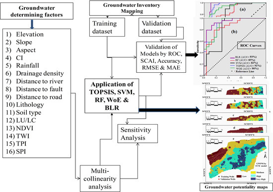
2.2. Methodology
2.3. Data Preparation
2.3.1. Groundwater Inventory Map (GWIM)
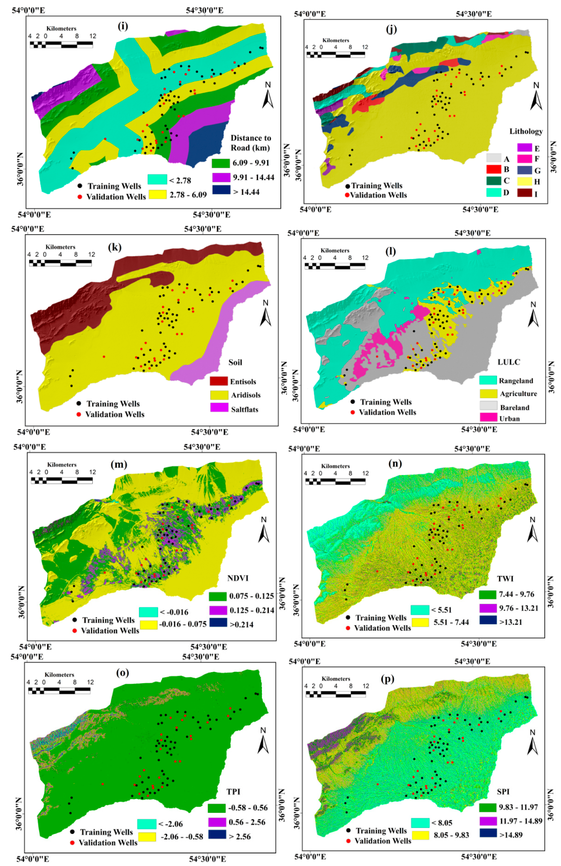
2.3.2. Groundwater Determining Factors (GWDFs)
2.4. Models
2.4.1. Weight of Evidence (WoE) Model
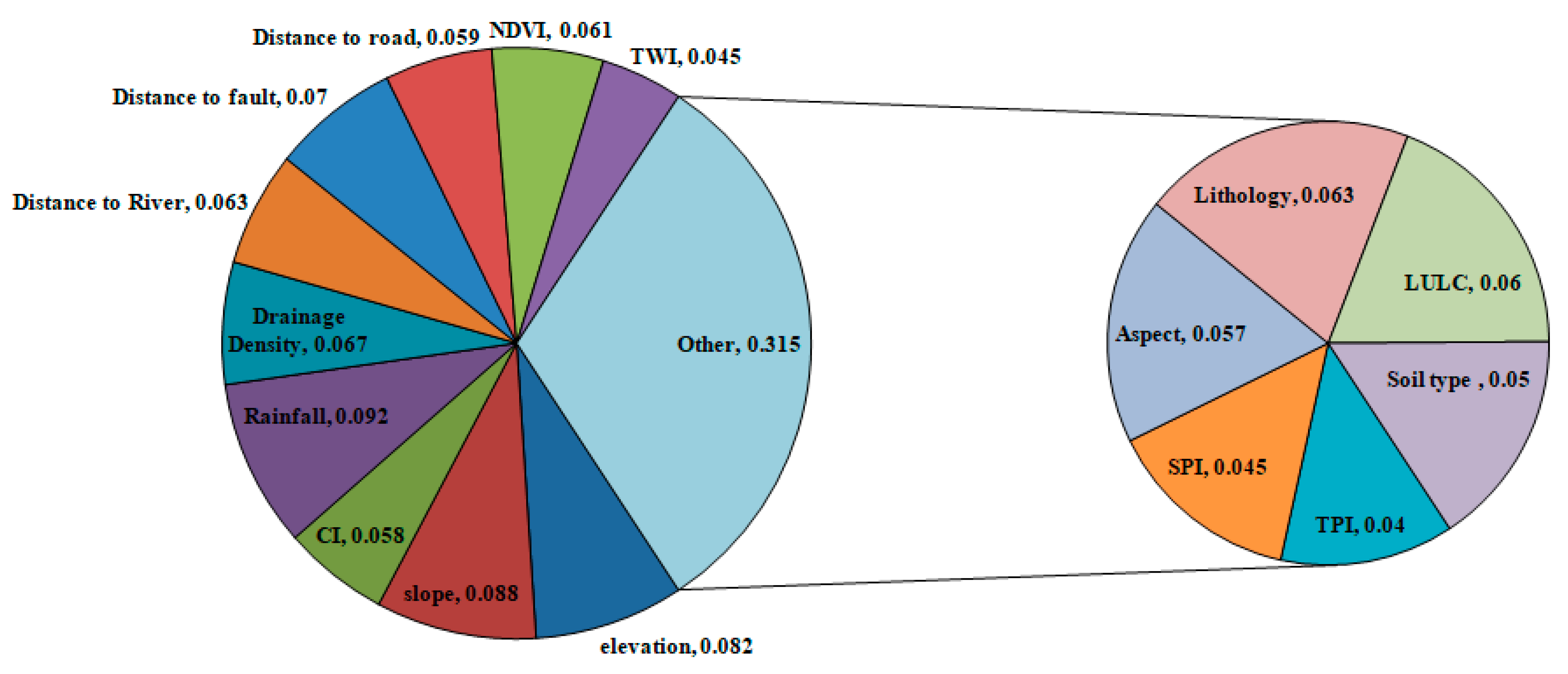
2.4.2. Random Forest (RF)
2.4.3. Binary Logistic Regression (BLR)
2.4.4. Technique for Order Preference by Similarity to Ideal Solution (TOPSIS)
2.4.5. Support Vector Machine (SVM)
2.5. Validation of Models
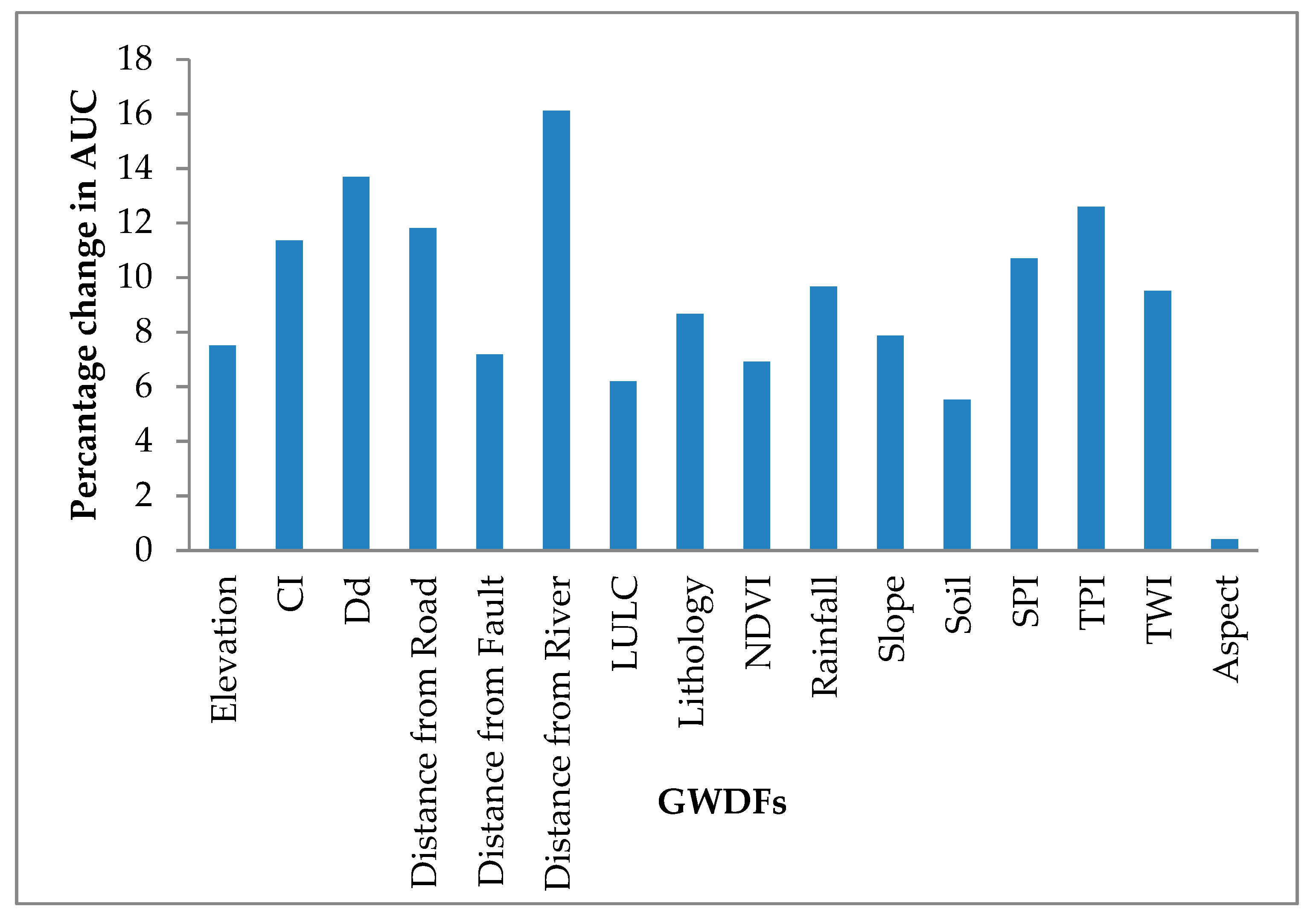
2.6. Sensitivity Analysis (SA)
3. Results
3.1. Analyzing the Multi-Collinearity (MC) of Groundwater Determining Factors
3.2. Application of the Weight of Evidence (WoE)
3.3. Application of Random Forest (RF) Model
3.4. Application of Binary Logistic Regression (BLR)
3.5. Application of TOPSIS
3.6. Application of Support Vector Machine (SVM)
3.7. Validations and Comparison of Models
3.8. Sensitivity Analysis
4. Discussion
5. Conclusions
Author Contributions
Funding
Conflicts of Interest
References
- Berhanu, B.; Seleshi, Y.; Melesse, A.M. Surface Water and Groundwater Resources of Ethiopia: Potentials and Challenges of Water Resources Development; Springer: Dordrecht, The Netherlands, 2014; pp. 97–117. [Google Scholar]
- Zehtabian, G.; Khosravi, H.; Ghodsi, M. High demand in a land of water scarcity: Iran. In Water and Sustainability in Arid Regions, 1st ed.; Graciela, S.M., Courel, M.F., Eds.; Springer: Dordrecht, The Netherlands, 2001; pp. 75–86. [Google Scholar]
- Manap, M.A.; Nampak, H.; Pradhan, B.; Lee, S.; Sulaiman, W.N.A.; Ramli, M.F. Application of probabilistic-based frequency ratio model in groundwater potential mapping using remote sensing data and GIS. Arab. J. Geosci. 2012, 7, 711–724. [Google Scholar] [CrossRef]
- National Geography Society. National Geographic, Almanac of Geography; National Geographic Books; National Geography Society: Washington, DC, USA, 2005. [Google Scholar]
- Jha, M.K.; Kamii, Y.; Chikamori, K. Cost-effective approaches for sustainable groundwater management in alluvial aquifer systems. Water Resour. Manag. 2009, 23, 219. [Google Scholar] [CrossRef]
- Gholizadeh, M.H.; Melesse, A.M.; Reddi, L. A comprehensive review on water quality parameters estimation using remote sensing techniques. Sensors 2016, 16, 1298. [Google Scholar] [CrossRef] [PubMed] [Green Version]
- Razandi, Y.; Pourghasemi, H.R.; SamaniNeisani, N.; Rahmati, O. Application of analytical hierarchy process, frequency ratio, and certainty factor models for groundwater potential mapping using GIS. Earth Sci. Inf. 2015, 8, 867–883. [Google Scholar] [CrossRef]
- Management and Planning Organization (MPO). Water Resources State Report; Management and Planning Organization (MPO): Tehran, Iran, 2004. [Google Scholar]
- Nosrati, K.; Eeckhaut, M.V.D. Assessment of groundwater quality usingmultivariate statistical techniques in Hashtgerd Plain, Iran. Environ. Earth Sci. 2012, 65, 331–344. [Google Scholar] [CrossRef]
- Rahmati, O.; Nazari Samani, A.; Mahdavi, M.; Pourghasemi, H.R.; Zeinivand, H. Groundwater potential mapping at Kurdistan region of Iran using analytic hierarchy process and GIS. Arab. J. Geosci. 2014, 8, 7059–7071. [Google Scholar] [CrossRef]
- Haghizadeh, A.; DavoudiMoghadam, D.; Pourghasemi, H.R. GIS-based bivariate statistical techniques for groundwater potential analysis (an example of Iran). J. Earth Syst. Sci. 2017, 126, 109. [Google Scholar] [CrossRef] [Green Version]
- Agarwal, R.; Garg, P.K. Remote sensing and GIS based groundwater potential & recharge zonesmapping using multi criteria decision making technique. Water Resour. Manag. 2016, 30, 243–260. [Google Scholar]
- Kharazmi, R.; Tavili, A.; Rahdari, M.R.; Chaban, L.; Panidi, E.; Rodrigo-Comino, J. Monitoring and assessment of seasonal land cover changes using remote sensing: A 30-year (1987–2016) case study of Hamoun Wetland, Iran. Environ. Monit. Assess. 2018, 190, 356. [Google Scholar] [CrossRef]
- He, B.; Wang, H.; Huang, L.; Liu, J.; Chen, Z. A new indicator of ecosystem water use efficiency based on surface soil moisture retrieved from remote sensing. Ecol. Indic. 2017, 75, 10–16. [Google Scholar] [CrossRef] [Green Version]
- Thilagavathi, N.; Subramani, T.; Suresh, M.; Karunanidhi, D. Mapping of groundwater potential zones in Salem Chalk Hills, Tamil Nadu, India, using remote sensing and GIS techniques. Environ. Monit. Assess. 2015, 187, 1–17. [Google Scholar] [CrossRef] [PubMed]
- Kordestani, M.D.; Naghibi, S.A.; Hashemi, H.; Ahmadi, K.; Kalantar, B.; Pradhan, B. Groundwater potential mapping using a novel data-mining ensemble model. Hydrogeol. J. 2018, 27, 211–224. [Google Scholar] [CrossRef] [Green Version]
- Golkarian, A.; Naghibi, S.A.; Kalantar, B.; Pradhan, B. Groundwater potential mapping using C5.0, random forest, and multivariate adaptive regression spline models in GIS. Environ. Monit. Assess. 2018, 190, 149. [Google Scholar] [CrossRef] [PubMed]
- Chen, W.; Li, H.; Hou, E.; Wang, S.; Wang, G.; Panahi, M. GIS-based groundwater potential analysis using novel ensemble weights-of-evidence with logistic regression and functional tree models. Sci. Total Environ. 2018, 1, 853–867. [Google Scholar] [CrossRef] [PubMed] [Green Version]
- Golkarian, A.; Rahmati, O. Use of a maximum entropy model to identify the key factors that influence groundwater availability on the Gonabad Plain, Iran. Environ. Earth Sci. 2018, 77, 369. [Google Scholar] [CrossRef]
- Saha, S. Groundwater potential mapping using analytical hierarchical process: A study on Md. Bazar Block of Birbhum District, West Bengal. Spat. Inf. Res. 2017, 25, 615–626. [Google Scholar] [CrossRef]
- Rahmati, O.; Naghibi, S.A.; Shahabi, H.; Tien Bui, D.; Pradhan, B.; Aareh, A.; Rafiei-Sardooi, E.; Samani, A.N.; Melesse, A.M. Groundwater spring potential modelling: Comprising the capability and robustness of three different modeling approaches. Hydrology 2018, 565, 248–261. [Google Scholar] [CrossRef]
- Naghibi, S.A.; Pourghasemi, H.R.; Abbaspour, K. A comparison between ten advanced and soft computing models for groundwater qanat potential assessment in Iran using R and GIS. Appl. Clim. 2018, 131, 967–984. [Google Scholar] [CrossRef]
- Arabameri, A.; Pourghasemi, H.R.; Cerda, A. Erodibility prioritization of subwatersheds using morphometric parameters analysis and its mapping: A comparison among TOPSIS, VIKOR, SAW, and CF multi-criteria decision making models. Sci. Total Environ. 2017, 613, 1385–1400. [Google Scholar]
- Arabameri, A.; Pourghasemi, H.R.; Yamani, M. Applying different scenarios for landslide spatial modeling using computational intelligence methods. Environ. Earth Sci. 2017, 76, 832. [Google Scholar] [CrossRef]
- Arabameri, A.; Pradhan, B.; Pourghasemi, H.R.; Rezaei, K.; Kerle, N. Spatial modeling of gully erosion using GIS and R programing: A comparison among three data mining algorithms. Appl. Sci. 2018, 8, 1369. [Google Scholar] [CrossRef] [Green Version]
- Arabameri, A.; Rezaei, K.; Pourghasemi, H.R.; Lee, S.; Yamani, M. GIS-based gully erosion susceptibility mapping: A comparison among three data-driven models and AHP knowledge-based technique. Environ. Earth Sci. 2018, 77, 628. [Google Scholar] [CrossRef]
- Islamic republic of Iran Meteorological Organization (IRIMO). 2012. Available online: http://www. semnanmet.ir (accessed on 12 August 2018).
- Tang, Q.; Hu, H.; Oki, T. Groundwater recharge and discharge in a hyperarid alluvial plain (Akesu, Taklimakan Desert, China). Hydrol. Processes 2007, 21, 1345–1353. [Google Scholar] [CrossRef]
- Geology Survey of Iran (GSI). 1997. Available online: http://www.gsi.ir/Main/Lang_en/index.html (accessed on 12 August 2018).
- Tehran Regional Water Cooperative (TRWC) Company. Simulation Project for Optimum Excavation of Dasht-e-Damghan; Principal Office of Water Resources: Washington, DC, USA, 2000; p. 46. [Google Scholar]
- UNEP. A Survey of Methods for Groundwater Recharge in Arid and Semi-Arid Regions; UNEP/DEWA/RS: New York, NY, USA; Bilthoven, The Netherlands, 2002; pp. 5–10. [Google Scholar]
- Arabameri, A.; Rezaei, K.; Cerda, A.; Lombardo, L.; Rodrigo-Comino, J. GIS-based groundwater potential mapping in Shahroud plain, Iran. A comparison among statistical (bivariate and multivariate), data mining and MCDM approaches. Sci. Total Environ. 2019, 658, 160–177. [Google Scholar] [CrossRef] [PubMed]
- Jothibasu, A.; Anbazhagan, S. Modeling groundwater probability index in Ponnaiyar River basin of South India using analytic hierarchy process. Model. Earth Syst. Environ. 2016, 2, 109. [Google Scholar] [CrossRef] [Green Version]
- Kiss, R. Determination of drainage network in digital elevation model. Util. Limit. J. Hung. Geomath. 2004, 2, 16–29. [Google Scholar]
- Moore, I.D.; Grayson, R.B.; Ladson, A.R. Digital terrain modeling: A review of hydrological, geomorphological and biological applications. Hydrol. Processes 1991, 5, 3–30. [Google Scholar] [CrossRef]
- Beven, K.J.; Kirkby, M.J. A physically based, variable contributing area model of basin hydrology. Hydrol. Sci. Bull. 1979, 24, 43–69. [Google Scholar] [CrossRef] [Green Version]
- Conforti, M.; Aucelli, P.C.; Robustelli, G.; Scarciglia, F. Geomorphology and GIS analysis for mapping gully erosion susceptibility in the Turbolo stream catchment (Northern Calabria, Italy). Nat. Hazards 2011, 56, 881–898. [Google Scholar] [CrossRef]
- Gómez-Gutiérrez, A.; Conoscenti, C.; Angileri, S.E.; Rotigliano, E.; Schnabel, S. Using topographical attributes to evaluate gully erosion proneness (susceptibility) in two mediterranean basins: Advantages and limitations. Nat. Hazards 2015, 79, 291–314. [Google Scholar] [CrossRef]
- Gallant, J.C.; Wilson, J.P. Primary topographic attributes. In Terrain Analysis: Principles and Applications; Wilson, J.P., Gallant, J.C., Eds.; Wiley: New York, NY, USA, 2000; pp. 51–85. [Google Scholar]
- Grohmann, C.H.; Riccomini, C. Comparison of roving-window and search-windowtechniques for characterising landscape morphometry. Comput. Geosci. 2009, 35, 2164–2169. [Google Scholar] [CrossRef] [Green Version]
- Dahal, R.K.; Hasegawa, S.; Nonomura, A.; Yamanaka, M.; Masuda, T.; Nishino, K. GIS based weights-of-evidence modelling of rainfall-induced landslides in small catchments for landslide susceptibility mapping. Environ. Geol. 2008, 54, 311–324. [Google Scholar] [CrossRef]
- Armas, I. Weights of evidence method for landslide susceptibility mapping; Prahova Subcarpathians, Romania. Nat. Hazards 2012, 60, 937–950. [Google Scholar] [CrossRef]
- Breiman, L. Random Forests. Mach. Learn. 2001, 45, 5–32. [Google Scholar] [CrossRef] [Green Version]
- Micheletti, N.; Foresti, L.; Robert, S.; Leuenberger, M.; Pedrazzini, A.; Jaboyedoff, M.; Kanevski, M. Machine learning feature selection methods for landslide susceptibility mapping. Math. Geosci. 2014, 46, 33–57. [Google Scholar] [CrossRef] [Green Version]
- Strobl, C.; Boulesteix, A.L.; Kneib, T.; Augustin, T.; Zeileis, A. Conditional variable importance for random forests. BMC Bioinf. 2008, 9, 307. [Google Scholar] [CrossRef] [Green Version]
- Caruana, R.; Niculescu-Mizil, A. An empirical comparison of supervised learning algorithms. In Proceedings of the 23rd International Conference on Machine Learning, Pittsburgh, PA, USA, 25–29 June 2006; ACM: New York, NY, USA, 2006; pp. 161–168. [Google Scholar]
- Reif, D.M.; Motsinger, A.A.; McKinney, B.A.; Crowe, J.E.; Moore, J.H. Feature Selection using a random forests classifier for the integrated analysis of multiple data type. In Proceedings of the 2006 IEEE Symposium on Computational Intelligence and Bioinformatics and Computational Biology, Toronto, ON, Canada, 28–29 September 2006. [Google Scholar]
- Kuhnert, P.M.; Henderson, A.K.; Bartley, R.; Herr, A. Incorporating uncertainty in gully erosion calculations using the random forests modelling approach. Environmetrics 2010, 21, 493–509. [Google Scholar] [CrossRef]
- Van Beijma, S.; Comber, A.; Lamb, A. Random forest classification of salt marsh vegetation habitats using quadpolarimetric airborne SAR, elevation and optical RS data. Remote Sens. Environ. 2014, 149, 118–129. [Google Scholar] [CrossRef]
- Archer, K.J.; Kimes, R.V. Empirical characterization of random forest variable importance measures. Comput. Stat. Data Anal. 2008, 52, 2249–2260. [Google Scholar] [CrossRef]
- R Development Core Team. R: A Language and Environment for Statistical Computing; R Foundation for Statistical Computing: Vienna, Austria, 2015; Available online: http://www.Rproject.org (accessed on 12 August 2018).
- Lombardo, L.; Opitz, T.; Huser, R. Point process-based modeling of multiple debris flow landslides using INLA: An application to the 2009 Messina disaster. Stoch. Environ. Res. Risk A 2018, 32, 2179–2198. [Google Scholar] [CrossRef] [Green Version]
- Hwang, C.L.; Yoon, K.P. Multiple Attribute Decision Making: Methods and Applications, 1st ed.; Springer: Berlin/Heidelberg, Germany, 1981. [Google Scholar]
- Zhang, Y.; Xu, Z. Efficiency evaluation of sustainable water management using the HF-TODIM method. Int. Trans. Op. Res. 2019, 26, 747–764. [Google Scholar] [CrossRef]
- Vomm, V.B. TOPSIS with statistical distances: A new approach to MADM. Decis. Sci. Lett. 2017, 6, 49–66. [Google Scholar] [CrossRef]
- Saaty, T.L. The Analytic Hierarchy Process; McGraw Hill: New York, NY, USA, 1980. [Google Scholar]
- Saaty, T.L. Fundamentals of Decision Making and Priority Theory with the Analytic Hierarchy Process; RWS Publications: Pittsburgh, PA, USA, 2000. [Google Scholar]
- Lootsma, F.A. Multi-Criteria Decision Analysis via Ratio and Difference Judgement, 1st ed.; Springer: New York, NY, USA, 2007. [Google Scholar]
- Bai, S.B.; Wang, J.; Lu, G.N.; Kanevski, M.; Pozdnoukhov, A. GIS based landslide susceptibility mapping with comparisons of results from machine learning methods process versus logistic regression in Bailongjiang river basin, China. Geophys. Res. Abstr. EGU 2008, 10, A-06367. [Google Scholar]
- Yao, X.; Tham, L.G.; Dai, F.C. Landslide susceptibility mapping based on support vector machine: A case study on natural slopes of Hong Kong, China. Geomorphology 2008, 101, 572–582. [Google Scholar] [CrossRef]
- Vapnik, V. Nature of Statistical Learning Theory; Wiley: New York, NY, USA, 1995. [Google Scholar]
- Tax, D.; Duin, E. Uniform object generation for optimizing one class classifiers. J. Mach. Learn. Res. 2002, 2, 155–173. [Google Scholar]
- Hastie, T.; Tibshirani, R.; Friedman, J. The Elements of Statistical Learning: Data Mining Inference and Prediction; Springer: New York, NY, USA, 2001. [Google Scholar]
- Pradhan, B. A comparative study on the predictive ability of the decision tree, support vector machine and neuro-fuzzy models in landslide susceptibility mapping using GIS. Comput. Geosci. 2013, 51, 350–365. [Google Scholar] [CrossRef]
- Camilo, D.C.; Lombardo, L.; Mai, P.M.; Dou, J.; Huser, R. Handling high predictor dimensionality in slope-unit-based landslide susceptibility models through LASSO penalized Generalized Linear Model. Environ. Model. Softw. 2018, 97, 145–156. [Google Scholar] [CrossRef] [Green Version]
- Yesilnacar, E.K. The Application of Computational Intelligence to Landslide Susceptibility Mapping in Turkey. Ph.D. Thesis, Department of Geomatics the University of Melbourne, Melbourne, Australia, 2005; p. 423. [Google Scholar]
- Süzen, M.L.; Doyuran, V. A comparison of the GIS based landslide susceptibility assessment methods: Multivariate versus bivariate. Environ. Geol. 2004, 45, 665–679. [Google Scholar] [CrossRef]
- Dao, D.V.; Trinh, S.H.; Ly, H.-B.; Pham, B.T. Prediction of Compressive Strength of Geopolymer Concrete Using Entirely Steel Slag Aggregates: Novel Hybrid Artificial Intelligence Approaches. Appl. Sci. 2019, 9, 1113. [Google Scholar] [CrossRef] [Green Version]
- Dao, D.V.; Ly, H.-B.; Trinh, S.H.; Le, T.-T.; Pham, B.T. Rtificial Intelligence Approaches for Prediction of Compressive Strength of Geopolymer Concrete. Materials 2019, 12, 983. [Google Scholar] [CrossRef] [Green Version]
- Ly, H.-B.; Monteiro, E.; Le, T.-T.; Le, V.M.; Dal, M.; Regnier, G. Prediction and Sensitivity Analysis of Bubble Dissolution Time in 3D Selective Laser Sintering Using Ensemble Decision Trees. Materials 2019, 12, 1544. [Google Scholar] [CrossRef] [PubMed] [Green Version]
- Pham, B.T.; Nguyen, M.D.; Bui, K.-T.T.; Prakash, I.; Chapi, K.; Bui, D.T. A novel artificial intelligence approach based on Multi-layer Perceptron Neural Network and Biogeography-based Optimization for predicting coefficient of consolidation of soil. Catena 2019, 173, 302–311. [Google Scholar] [CrossRef]
- Pham, B.T. A novel classifier based on composite hyper-cubes on iterated random projections for assessment of landslide susceptibility. J. Geol. Soc. India 2018, 91, 355–362. [Google Scholar] [CrossRef]
- Saltelli, A.; Chan, K.; Scott, E.M. Sensitivity Analysis; Wiley: New York, NY, USA, 2000. [Google Scholar]
- Refsgaard, J.C.; Sluijs, J.P.V.D.; Højberg, A.L.; Vanrolleghem, P.A. Uncertainty in the environmental modelling process—A framework and guidance. Water Resour. Manag. 2007, 22, 1543–1556. [Google Scholar] [CrossRef] [Green Version]
- Crosetto, M.; Tarantola, S. Uncertainty and sensitivity analysis: Tools for GIS-based model implementation. Int. J. Geogr. Inf. Sci. 2001, 15, 415–437. [Google Scholar] [CrossRef]
- Ferretti, F.; Saltelli, A.; Tarantola, S. Trends in sensitivity analysis practice in the last decade. Sci. Total Environ. 2016, 568, 666–670. [Google Scholar] [CrossRef]
- Chen, Y.; Yu, J.; Khan, S. Spatial sensitivity analysis of multi-criteria weights in GIS-based land suitability evaluation. Environ. Model. Softw. 2010, 25, 1582–1591. [Google Scholar] [CrossRef]
- Lodwick, W.A.; Monson, W.; Svoboda, L. Attribute error and sensitivity analysis of map operations in geographical information systems: Suitability analysis. Int. J. Geogr. Inf. Syst. 1990, 4, 413–428. [Google Scholar] [CrossRef]
- Oh, H.J.; Kim, Y.S.; Choi, J.K.; Park, E.; Lee, S. GIS mapping of regional probabilistic groundwater potential in the area of Pohang City, Korea. J. Hydrol. 2011, 399, 158–172. [Google Scholar] [CrossRef]
- Fenta, A.A.; Kifle, A.; Gebreyohannes, T.; Hailu, G. Spatial analysis of groundwater potential using remote sensing and GIS-based multi-criteria evaluation in Raya Valley, northern Ethiopia. Hydrogeol. J. 2015, 23, 195–206. [Google Scholar] [CrossRef]
- Tahmassebipoor, N.; Rahmati, O.; Noormohamadi, F.; Lee, S. Spatial analysis of groundwater potential using weights-of-evidence and evidential belief function models and remote sensing. Arab. J. Geosci. 2016, 9, 1–18. [Google Scholar] [CrossRef]
- Convertino, M.; Muñoz-Carpena, R.; Chu-Agor, M.L.; Kiker, G.L.; Linkov, I. Untangling drivers of species distributions: Global sensitivity and uncertainty analyses of MAXENT. Environ. Model. Softw. 2014, 51, 296–309. [Google Scholar] [CrossRef]
- Park, N.W. Using maximum entropymodeling for landslide susceptibility mapping with multiple geoenvironmental data sets. Environ. Earth Sci. 2015, 73, 937–949. [Google Scholar] [CrossRef]
- Tien Bui, D.; Lofman, O.; Revhaug, I.; Dick, O. Landslide susceptibility analysis in the Hoa Binh province of Vietnamusing statistical index and logistic regression. Nat. Hazards 2011, 59, 1413–1444. [Google Scholar]
- Cama, M.; Lombardo, L.; Conoscenti, C.; Rotigliano, E. Improving transferability strategies for debris flow susceptibility assessment. Application to the Saponara and Itala catchments (Messina, Italy). Geomorphology 2017, 288, 52–65. [Google Scholar] [CrossRef]
- Chen, W.; Xie, X.; Wang, J.; Pradhan, B.; Hong, H.; Bui, D.T. A comparative study of logistic model tree, random forest, and classification and regression tree models for spatial prediction of landslide susceptibility. Catena 2017, 151, 147–160. [Google Scholar] [CrossRef] [Green Version]
- Roy, J.; Saha, S. Landslide susceptibility mapping using knowledge driven statistical models in Darjeeling District, West Bengal, India. Geoenvironmental Disasters 2019, 6, 11. [Google Scholar] [CrossRef] [Green Version]
- Regmi, N.R.; Giardino, J.R.; Vitek, J.D. Modeling susceptibility to landslides using the weight of evidence approach: Western Colorado, USA. Geomorphology 2010, 115, 172–187. [Google Scholar] [CrossRef]
- Moghaddam, D.D.; Rezaei, M.; Pourghasemi, H.R.; Pourtaghie, Z.S.; Pradhan, B. Groundwater spring potential mapping using bivariate statistical model and GIS in the Taleghan Watershed, Iraq. Arab. J. Geosci. 2013, 8, 913–929. [Google Scholar] [CrossRef]
- Pope, A.; Murray, T.; Luckman, A. DEM quality assessment for quantification of glacier surface change. Ann. Glaciol. 2014, 46, 189–194. [Google Scholar] [CrossRef] [Green Version]
- Erasmi, S.; Rosenbauer, R.; Buchbach, R.; Busche, T.; Rutishauser, S. Evaluating the quality and accuracy of TanDEM-X digital elevation models at archaeological sites in the Cilician Plain, Turkey. Remote Sens. 2014, 6, 9475–9493. [Google Scholar] [CrossRef] [Green Version]
- Blaschke, T. Object based image analysis for remote sensing. ISPRS J. Photogramm. Remote Sens. 2010, 65, 2–16. [Google Scholar] [CrossRef] [Green Version]
- Alganci, U.; Besol, B.; Sertel, E. Accuracy assessment of different digital surface models. ISPRS Int. J. Geo-Inf. 2018, 7, 114. [Google Scholar] [CrossRef] [Green Version]
- Mohammady, M.; Pourghasemi, H.R.; Pradhan, B. Landslide susceptibility mapping at Golestan Province, Iran: A comparison between frequency ratio, Dempster–Shafer, and weights-of-evidence models. J. Asian Earth Sci. 2012, 61, 221–236. [Google Scholar] [CrossRef]
- Tehrany, M.S.; Pradhan, B.; Jebur, M.N. Spatial prediction of flood susceptible areas using rule based decision tree (DT) and a novel ensemble bivariate and multivariate statistical models in GIS. J. Hydrol. 2013, 504, 69–79. [Google Scholar] [CrossRef]
- Hong, H.; Tsangaratos, P.; Ilia, L.; Chen, W.; Xu, C. Comparing the performance of a logistic regression and a random forest model in landslide susceptibility assessments. The Case of Wuyaun Area, China. In Proceedings of the Workshop World Landslide Forum, Ljubljana, Slovenia, 29 May–2 June 2017; pp. 1043–1050. [Google Scholar]
- Hemasinghe, H.; Rangali, R.S.S.; Deshapriya, N.L.; Samarakoon, L. Landslide susceptibility mapping using logistic regression model (a case study in Badulla District, Sri Lanka). Procedia Eng. 2018, 212, 1046–1053. [Google Scholar] [CrossRef]


| Group | Unit | Description |
|---|---|---|
| A | COm | Dolomite platy and flaggy limestone containing trilobite; sandstone and shale (MILA FM). |
| Cl | Dark red medium-grained arkosic to subarkosic sandstone and micaceous siltstone (LALUN FM). | |
| B | DCkh | Yellowish, thin to thick-bedded, fossiliferous argillaceous limestone, dark grey limestone, greenish marl and shale, locally including gypsum |
| Db | Grey and black, partly nodular limestone with intercalations of calcareous shale (BAHRAM FM). | |
| C | E1s | Sandstone, conglomerate, marl and sandy limestone. |
| Ek | Well bedded green tuff and tuffaceous shale (KARAJ FM). | |
| D | Jl | Light grey, thin-bedded to massive limestone (LAR FM). |
| E | K2m,l | Marl, shale and detritic limestone. |
| K | Cretaceous rocks in general. | |
| F | Murmg | Gypsiferous marl. |
| Murc | Red conglomerate and sandstone. | |
| G | Plc | Polymictic conglomerate and sandstone. |
| PlQc | Fluvial conglomerate, Piedmont conglomerate and sandstone. | |
| P | Undifferentiated Permian rocks. | |
| Pr | Dark grey medium-bedded to massive limestone (RUTEH LIMESTONE). | |
| H | Qft2 | Low level piedmont fan and valley terrace deposits. |
| Qft1 | High level piedmont fan and valley terrace deposits. | |
| Qcf | Clay flat. | |
| Qal | Stream channel, braided channel and flood plain deposits. | |
| I | TRJs | Dark grey shale and sandstone (SHEMSHAK FM). |
| Factors | Min. | Max. | Classes | Methods |
|---|---|---|---|---|
| Elevation (m) | 1043 | 2869 | (1.) <1155, (2.) 1155 –1297, (3.) 1297–1512, (4.) 1512–1993, (5.) >1993 | Natural break (Jenks) |
| Slope (degree) | 0 | 72.32 | (1.) <2.55, (2.) 2.55–9.35, (3.) 9.35–20.70, (4.) 20.70–34.03, (5.) >34.03 | Natural break (Jenks) |
| Aspect | - | - | (1.) Flat (−1), (2.) North (0–22.5), (3.) Northeast (22.5–67.5), (4.) East (67.5–112.5), (5.) Southeast (112.5–157.5), (6.) South (157.5–202.5), (7.) Southwest (202.5–247.5), (8.) West (247.5–292.5), (9.) Northwest (292.5–337.5) | Directional units |
| Convergence index | -100 | 100 | (1.) <−59.21, (2.) −59.21–-18.43, (3.) −18.43–17.64, (4.) 17.64–57.64, (5.) >57.64 | Natural break (Jenks) |
| Rainfall (mm) | 96 | 406 | (1.) <132.95, (2.) 132.95–170.69, (3.) 170.69–226.68, (4.) 226.68–305.81, (5.) >305.81 | Natural break (Jenks) |
| Lithology | - | - | (1.) A, (2.) B, (3.) C, (4.) D, (5.) E, (6.) F, (7.) G, (8.) H, (9.) I | Lithological Units |
| Soil type | - | - | (1.) Aridisols, (2.) Rock outcrops/entisols, (3.) Salt flats | Soil types/ Orders |
| LULC | - | - | (1.) Bare land, (2.) Agriculture land, (3.) Rangeland, (4.) Urban | Supervised Classification |
| Drainage density (km/km2) | 0.15 | 3.18 | (1.) <1.12, (2.) 1.12 –1.54, (3.) 1.54–1.88, (4.) 1.88–2.24, (5.) >2.24 | Natural break (Jenks) |
| Distance to river (km) | 0 | 1.35 | (1.) <0.10, (2.) 0.10–0.21, (3.) 0.21–0.37, (4.) 0.37–0.57, (5.) >0.57 | Natural break (Jenks) |
| Distance to fault (km) | 0 | 16.08 | (1.) <2.20, (2.) 2.20–4.85, (3.) 4.85–7.75, (4.) 7.75–10.91, (5.) >10.91 | Natural break (Jenks) |
| Distance to road (km) | 0 | 22.18 | (1.) <2.78, (2.) 2.78–6.09, (3.) 6.09–9.91, (4.) 9.91–14.44, (5.) >14.44 | Natural break (Jenks) |
| NDVI | −0.24 | 0.54 | (1.) <−0.01, (2.) −0.01–0.07, (3.) 0.07–0.12, (4.) 0.12–0.21, (5.) >0.21 | Natural break (Jenks) |
| TWI | 1.11 | 21.54 | (1.) <5.51, (2.) 5.51–7.44, (3.) 7.44–9.76, (4.) 9.76–13.21, (5.) >13.21 | Natural break (Jenks) |
| TPI | −12.16 | 14.67 | (1.) <−2.06, (2.) −2.06–−0.58, (3.) −0.58–0.56, (4.) 0.56–2.56, (5.) >2.56 | Natural break (Jenks) |
| SPI | 6.27 | 24.44 | (1.) <8.05, (2.) 8.05–9.83, (3.) 9.83–11.97, (4.) 11.97–14.89, (5.) >14.89 | Natural break (Jenks) |
| AUC Values | Accuracy Statements |
|---|---|
| 0.5–0.6 | Low |
| 0.6–0.7 | Moderate |
| 0.7–0.8 | High |
| 0.8–0.9 | Very high |
| 0.9–1 | Excellent |
| Conditioning Factors | Collinearity Statistics | |
|---|---|---|
| Tolerance | VIF | |
| Elevation | 0.281 | 4.275 |
| Slope | 0.256 | 3.908 |
| Convergence Index | 0.816 | 1.226 |
| Rainfall | 0.202 | 4.792 |
| Drainage Density | 0.542 | 1.846 |
| Distance to River | 0.855 | 1.170 |
| Distance to Fault | 0.527 | 1.897 |
| Distance to Road | 0.485 | 2.061 |
| NDVI | 0.704 | 1.420 |
| TWI | 0.201 | 4.911 |
| TPI | 0.891 | 1.122 |
| SPI | 0.202 | 4.713 |
| Aspect | 0.916 | 1.092 |
| Lithology | 0.580 | 1.724 |
| LULC | 0.612 | 1.634 |
| Soil Type | 0.492 | 2.032 |
| Elevation (m) | Pixels | % of Pixel | Well | % of Well | W+ | W− | C | S2W+ | S2W− | S© | C/S© |
|---|---|---|---|---|---|---|---|---|---|---|---|
| <1043–1155 | 855,560 | 49.36 | 53 | 94.64 | 0.65 | −2.25 | 2.90 | 0.02 | 0.33 | 0.59 | 4.88 |
| 1155–1297 | 446,173 | 25.74 | 3 | 5.36 | −1.57 | 0.24 | −1.81 | 0.33 | 0.02 | 0.59 | −3.05 |
| 1297–1512 | 303,221 | 17.50 | 0 | 0.00 | 0.00 | 0.19 | 0.00 | 0.00 | 0.02 | 0.00 | 0.00 |
| 1512–1993 | 101,149 | 5.84 | 0 | 0.00 | 0.00 | 0.06 | 0.00 | 0.00 | 0.02 | 0.00 | 0.00 |
| >1993 | 27,036 | 1.56 | 0 | 0.00 | 0.00 | 0.02 | 0.00 | 0.00 | 0.02 | 0.00 | 0.00 |
| Slope (degree) | |||||||||||
| <2.55 | 126,724,5 | 73.12 | 55 | 98.21 | 0.30 | −2.71 | 3.01 | 0.02 | 1.00 | 1.01 | 2.98 |
| 2.55–9.35 | 335,864 | 19.38 | 1 | 1.79 | −2.38 | 0.20 | −2.58 | 1.00 | 0.02 | 1.01 | −2.56 |
| 9.35–20.70 | 638,68 | 3.69 | 0 | 0.00 | 0.00 | 0.04 | 0.00 | 0.00 | 0.02 | 0.00 | 0.00 |
| 20.70–34.03 | 44,815 | 2.59 | 0 | 0.00 | 0.00 | 0.03 | 0.00 | 0.00 | 0.02 | 0.00 | 0.00 |
| >34.03 | 21,347 | 1.23 | 0 | 0.00 | 0.00 | 0.01 | 0.00 | 0.00 | 0.02 | 0.00 | 0.00 |
| Aspect | |||||||||||
| F | 82,884 | 4.78 | 3 | 5.36 | 0.11 | −0.01 | 0.12 | 0.33 | 0.02 | 0.59 | 0.20 |
| N | 89,279 | 5.15 | 3 | 5.36 | 0.04 | 0.00 | 0.04 | 0.33 | 0.02 | 0.59 | 0.07 |
| NE | 154,448 | 8.91 | 9 | 16.07 | 0.59 | −0.08 | 0.67 | 0.11 | 0.02 | 0.36 | 1.85 |
| E | 296,877 | 17.13 | 10 | 17.86 | 0.04 | −0.01 | 0.05 | 0.10 | 0.02 | 0.35 | 0.14 |
| SE | 431,538 | 24.90 | 8 | 14.29 | −0.56 | 0.13 | −0.69 | 0.13 | 0.02 | 0.38 | −1.80 |
| S | 359,878 | 20.76 | 12 | 21.43 | 0.03 | −0.01 | 0.04 | 0.08 | 0.02 | 0.33 | 0.12 |
| SW | 167,965 | 9.69 | 7 | 12.50 | 0.25 | −0.03 | 0.29 | 0.14 | 0.02 | 0.40 | 0.71 |
| W | 853,21 | 4.92 | 3 | 5.36 | 0.08 | 0.00 | 0.09 | 0.33 | 0.02 | 0.59 | 0.15 |
| NW | 64,949 | 3.75 | 1 | 1.79 | −0.74 | 0.02 | −0.76 | 1.00 | 0.02 | 1.01 | −0.75 |
| Convergence Index | |||||||||||
| <−59.21568627 | 145,566 | 8.40 | 9 | 16.07 | 0.65 | −0.09 | 0.74 | 0.11 | 0.02 | 0.36 | 2.02 |
| −59.21–−18.43 | 368,782 | 21.28 | 14 | 25.00 | 0.16 | −0.05 | 0.21 | 0.07 | 0.02 | 0.31 | 0.68 |
| −18.43–17.64 | 707,982 | 40.85 | 14 | 25.00 | −0.49 | 0.24 | −0.73 | 0.07 | 0.02 | 0.31 | −2.36 |
| 17.64–57.64 | 364,974 | 21.06 | 10 | 17.86 | −0.16 | 0.04 | −0.20 | 0.10 | 0.02 | 0.35 | −0.59 |
| >57.64 | 145,835 | 8.41 | 9 | 16.07 | 0.65 | −0.09 | 0.73 | 0.11 | 0.02 | 0.36 | 2.02 |
| Rainfall (mm) | |||||||||||
| <132 | 429,194 | 24.76 | 22 | 39.29 | 0.46 | −0.21 | 0.68 | 0.05 | 0.03 | 0.27 | 2.47 |
| 132–170 | 100,66,02 | 58.08 | 34 | 60.71 | 0.04 | −0.06 | 0.11 | 0.03 | 0.05 | 0.27 | 0.40 |
| 170–226 | 166,770 | 9.62 | 0 | 0.00 | 0.00 | 0.10 | 0.00 | 0.00 | 0.02 | 0.00 | 0.00 |
| 226–305 | 77,365 | 4.46 | 0 | 0.00 | 0.00 | 0.05 | 0.00 | 0.00 | 0.02 | 0.00 | 0.00 |
| >305 | 53,208 | 3.07 | 0 | 0.00 | 0.00 | 0.03 | 0.00 | 0.00 | 0.02 | 0.00 | 0.00 |
| Lithology | |||||||||||
| A | 7093 | 0.41 | 0 | 0.00 | 0.00 | 0.00 | 0.00 | 0.00 | 0.02 | 0.00 | 0.00 |
| B | 35,899 | 2.07 | 0 | 0.00 | 0.00 | 0.02 | 0.00 | 0.00 | 0.02 | 0.00 | 0.00 |
| C | 57,180 | 3.30 | 0 | 0.00 | 0.00 | 0.03 | 0.00 | 0.00 | 0.02 | 0.00 | 0.00 |
| D | 72,339 | 4.17 | 0 | 0.00 | 0.00 | 0.04 | 0.00 | 0.00 | 0.02 | 0.00 | 0.00 |
| E | 23,837 | 1.38 | 0 | 0.00 | 0.00 | 0.01 | 0.00 | 0.00 | 0.02 | 0.00 | 0.00 |
| F | 24,485 | 1.41 | 0 | 0.00 | 0.00 | 0.01 | 0.00 | 0.00 | 0.02 | 0.00 | 0.00 |
| G | 86,958 | 5.02 | 2 | 3.57 | −0.34 | 0.02 | −0.36 | 0.50 | 0.02 | 0.72 | −0.49 |
| H | 138,8009 | 80.09 | 54 | 96.43 | 0.19 | −1.72 | 1.90 | 0.02 | 0.50 | 0.72 | 2.64 |
| I | 37,340 | 2.15 | 0 | 0.00 | 0.00 | 0.02 | 0.00 | 0.00 | 0.02 | 0.00 | 0.00 |
| Aridisols | 118,6872 | 68.48 | 54 | 96.43 | 0.34 | −2.18 | 2.52 | 0.02 | 0.50 | 0.72 | 3.50 |
| Rock Outcrops/Entisols | 392,588 | 22.65 | 0 | 0.00 | 0.00 | 0.26 | 0.00 | 0.00 | 0.02 | 0.00 | 0.00 |
| Salt Flats | 153,679 | 8.87 | 2 | 3.57 | −0.91 | 0.06 | −0.97 | 0.50 | 0.02 | 0.72 | −1.34 |
| LULC | |||||||||||
| Bareland | 654,072 | 37.74 | 4 | 7.14 | −1.66 | 0.40 | −2.06 | 0.25 | 0.02 | 0.52 | −3.98 |
| Agriculture | 206,538 | 11.92 | 52 | 92.86 | 2.05 | −2.51 | 4.57 | 0.02 | 0.25 | 0.52 | 8.80 |
| Rangeland | 777,361 | 44.85 | 0 | 0.00 | 0.00 | 0.60 | 0.00 | 0.00 | 0.02 | 0.00 | 0.00 |
| Urban | 95,167 | 5.49 | 0 | 0.00 | 0.00 | 0.06 | 0.00 | 0.00 | 0.02 | 0.00 | 0.00 |
| Drainage Density (km/square km) | |||||||||||
| <1.12 | 125,010 | 7.21 | 0 | 0.00 | 0.00 | 0.07 | 0.00 | 0.00 | 0.02 | 0.00 | 0.00 |
| 1.12–1.54 | 360,107 | 20.78 | 6 | 10.71 | −0.66 | 0.12 | −0.78 | 0.17 | 0.02 | 0.43 | −1.81 |
| 1.54–1.88 | 480,396 | 27.72 | 19 | 33.93 | 0.20 | −0.09 | 0.29 | 0.05 | 0.03 | 0.28 | 1.03 |
| 1.88–2.24 | 452,295 | 26.10 | 20 | 35.71 | 0.31 | −0.14 | 0.45 | 0.05 | 0.03 | 0.28 | 1.62 |
| >2.24 | 315,331 | 18.19 | 11 | 19.64 | 0.08 | −0.02 | 0.09 | 0.09 | 0.02 | 0.34 | 0.28 |
| Distance to River (km) | |||||||||||
| <0.10 | 629,316 | 36.31 | 23 | 41.07 | 0.12 | −0.08 | 0.20 | 0.04 | 0.03 | 0.27 | 0.74 |
| 0.10–0.21 | 519,863 | 30.00 | 19 | 33.93 | 0.12 | −0.06 | 0.18 | 0.05 | 0.03 | 0.28 | 0.64 |
| 0.21–0.37 | 360,248 | 20.79 | 9 | 16.07 | −0.26 | 0.06 | −0.32 | 0.11 | 0.02 | 0.36 | −0.87 |
| 0.37–0.57 | 170,585 | 9.84 | 4 | 7.14 | −0.32 | 0.03 | −0.35 | 0.25 | 0.02 | 0.52 | −0.67 |
| >0.57 | 53,127 | 3.07 | 1 | 1.79 | −0.54 | 0.01 | −0.55 | 1.00 | 0.02 | 1.01 | −0.55 |
| Distance to Fault (km) | |||||||||||
| <2.20 | 634,007 | 36.58 | 7 | 12.50 | −1.07 | 0.32 | −1.40 | 0.14 | 0.02 | 0.40 | −3.45 |
| 2.20–4.85 | 339,860 | 19.61 | 12 | 21.43 | 0.09 | −0.02 | 0.11 | 0.08 | 0.02 | 0.33 | 0.34 |
| 4.85–7.75 | 295,667 | 17.06 | 14 | 25.00 | 0.38 | −0.10 | 0.48 | 0.07 | 0.02 | 0.31 | 1.56 |
| 7.75–10.91 | 272,734 | 15.74 | 18 | 32.14 | 0.71 | −0.22 | 0.93 | 0.06 | 0.03 | 0.29 | 3.25 |
| >10.91 | 190,871 | 11.01 | 5 | 8.93 | −0.21 | 0.02 | −0.23 | 0.20 | 0.02 | 0.47 | −0.50 |
| Distance to Road (km) | |||||||||||
| <2.78 | 584,777 | 33.74 | 22 | 39.29 | 0.15 | −0.09 | 0.24 | 0.05 | 0.03 | 0.27 | 0.88 |
| 2.78–6.09 | 503,128 | 29.03 | 24 | 42.86 | 0.39 | −0.22 | 0.61 | 0.04 | 0.03 | 0.27 | 2.25 |
| 6.09–9.91 | 341,304 | 19.69 | 8 | 14.29 | −0.32 | 0.07 | −0.39 | 0.13 | 0.02 | 0.38 | −1.01 |
| 9.91–14.44 | 216,429 | 12.49 | 2 | 3.57 | −1.25 | 0.10 | −1.35 | 0.50 | 0.02 | 0.72 | −1.87 |
| >14.44 | 87,501 | 5.05 | 0 | 0.00 | 0.00 | 0.05 | 0.00 | 0.00 | 0.02 | 0.00 | 0.00 |
| NDVI | |||||||||||
| <−0.01 | 946 | 0.05 | 0 | 0.00 | 0.00 | 0.00 | 0.00 | 0.00 | 0.02 | 0.00 | 0.00 |
| −0.0–0.07 | 995,879 | 57.46 | 8 | 14.29 | −1.39 | 0.70 | −2.09 | 0.13 | 0.02 | 0.38 | −5.48 |
| 0.07–0.12 | 614,296 | 35.44 | 28 | 50.00 | 0.34 | −0.26 | 0.60 | 0.04 | 0.04 | 0.27 | 2.24 |
| 0.12–0.21 | 95,540 | 5.51 | 15 | 26.79 | 1.58 | −0.26 | 1.84 | 0.07 | 0.02 | 0.30 | 6.08 |
| >0.21 | 26,478 | 1.53 | 5 | 8.93 | 1.77 | −0.08 | 1.84 | 0.20 | 0.02 | 0.47 | 3.93 |
| TWI | |||||||||||
| <5.51 | 315,821 | 18.22 | 0 | 0.00 | 0.00 | 0.20 | 0.00 | 0.00 | 0.02 | 0.00 | 0.00 |
| 5.51–7.44 | 793,998 | 45.81 | 32 | 57.14 | 0.22 | −0.23 | 0.46 | 0.03 | 0.04 | 0.27 | 1.69 |
| 7.44–9.76 | 391,225 | 22.57 | 14 | 25.00 | 0.10 | −0.03 | 0.13 | 0.07 | 0.02 | 0.31 | 0.43 |
| 9.76–13.21 | 174,040 | 10.04 | 8 | 14.29 | 0.35 | −0.05 | 0.40 | 0.13 | 0.02 | 0.38 | 1.05 |
| >13.21 | 58,055 | 3.35 | 2 | 3.57 | 0.06 | 0.00 | 0.07 | 0.50 | 0.02 | 0.72 | 0.09 |
| <−2.06 | 11,457 | 0.66 | 0 | 0.00 | 0.00 | 0.01 | 0.00 | 0.00 | 0.02 | 0.00 | 0.00 |
| −2.06–−0.58 | 55,078 | 3.18 | 0 | 0.00 | 0.00 | 0.03 | 0.00 | 0.00 | 0.02 | 0.00 | 0.00 |
| −0.58–0.56 | 160,7635 | 92.76 | 55 | 98.21 | 0.06 | −1.40 | 1.46 | 0.02 | 1.00 | 1.01 | 1.44 |
| 0.56–2.56 | 47,227 | 2.72 | 1 | 1.79 | −0.42 | 0.01 | −0.43 | 1.00 | 0.02 | 1.01 | −0.43 |
| >2.56 | 11,742 | 0.68 | 0 | 0.00 | 0.00 | 0.01 | 0.00 | 0.00 | 0.02 | 0.00 | 0.00 |
| SPI | |||||||||||
| <8.05 | 538,726 | 31.08 | 23 | 41.07 | 0.28 | −0.16 | 0.44 | 0.04 | 0.03 | 0.27 | 1.60 |
| 8.05–9.83 | 595,727 | 34.37 | 20 | 35.71 | 0.04 | −0.02 | 0.06 | 0.05 | 0.03 | 0.28 | 0.21 |
| 9.83− 11.97 | 329,339 | 19.00 | 6 | 10.71 | −0.57 | 0.10 | −0.67 | 0.17 | 0.02 | 0.43 | −1.55 |
| 11.97–14.89 | 171,410 | 9.89 | 4 | 7.14 | −0.33 | 0.03 | −0.36 | 0.25 | 0.02 | 0.52 | −0.69 |
| >14.89 | 95,996 | 5.54 | 3 | 5.36 | −0.03 | 0.00 | −0.04 | 0.33 | 0.02 | 0.59 | −0.06 |
| Models | Potentiality Classes | Area in Square km | % of Area |
|---|---|---|---|
| TOPSIS | Low | 446.1995 | 23.2 |
| Medium | 787.3882 | 40.94 | |
| High | 399.4639 | 20.77 | |
| Very high | 290.222 | 15.09 | |
| WoE | Low | 424.8511 | 22.09 |
| Medium | 617.3708 | 32.1 | |
| High | 583.9059 | 30.36 | |
| Very high | 297.3381 | 15.46 | |
| RF | Low | 1064.34 | 55.34 |
| Medium | 198.6742 | 10.33 | |
| High | 174.4409 | 9.07 | |
| Very high | 485.8189 | 25.26 | |
| BLR | Low | 744.3069 | 38.7 |
| Medium | 594.4839 | 30.91 | |
| High | 286.9524 | 14.92 | |
| Very high | 297.5304 | 15.47 | |
| SVM | Low | 248.6793 | 12.93 |
| Medium | 569.0967 | 29.59 | |
| High | 744.8839 | 38.73 | |
| Very high | 360.4215 | 18.74 |
| Observation | Predicted | Class Error | OOB (%) | |
|---|---|---|---|---|
| 0 | 1 | |||
| 0 | 8273 | 149 | 0.018 | 3.32 |
| 1 | 180 | 1319 | 0.120 | |
| Parameters | Weight |
|---|---|
| Elevation | 0.0237 |
| Slope | 0.5778 |
| CI | 0.0029 |
| Rainfall | 0.0131 |
| Drainage Density | −1.739 |
| Distance to River | −0.0008 |
| Distance to Fault | 0.0001 |
| Distance to Road | 0.0002 |
| NDVI | −7.633 |
| TWI | 0.2892 |
| TPI | 0.0426 |
| SPI | −0.1487 |
| Aspect | −1.3488 |
| Lithology | 2.5531 |
| LULC | 2.2942 |
| Soil types | 6.8088 |
| Training Dataset | Validation Dataset | |||||||||
|---|---|---|---|---|---|---|---|---|---|---|
| Measures | WoE | RF | TOPSIS | SVM | BLR | WoE | RF | TOPSIS | SVM | BLR |
| True positive | 46 | 44 | 45 | 42 | 46 | 20 | 17 | 20 | 18 | 20 |
| True negative | 45 | 45 | 47 | 45 | 48 | 19 | 19 | 21 | 19 | 22 |
| False positive | 10 | 12 | 11 | 12 | 10 | 4 | 6 | 4 | 6 | 4 |
| False negative | 11 | 11 | 9 | 11 | 8 | 5 | 5 | 3 | 5 | 2 |
| Sensitivity | 0.807 | 0.800 | 0.833 | 0.792 | 0.852 | 0.800 | 0.773 | 0.870 | 0.783 | 0.909 |
| Specificity | 0.818 | 0.789 | 0.810 | 0.789 | 0.828 | 0.826 | 0.760 | 0.840 | 0.760 | 0.846 |
| Accuracy | 0.813 | 0.795 | 0.821 | 0.791 | 0.839 | 0.813 | 0.766 | 0.854 | 0.771 | 0.875 |
| RMSE | 0.317 | 0.367 | 0.316 | 0.377 | 0.314 | 0.332 | 0.383 | 0.321 | 0.409 | 0.311 |
| MAE | 0.221 | 0.275 | 0.219 | 0.269 | 0.216 | 0.235 | 0.288 | 0.233 | 0.311 | 0.214 |
| AUC | 0.914 | 0.846 | 0.924 | 0.833 | 0.933 | 0.898 | 0.81 | 0.901 | 0.851 | 0.943 |
| Models | Groundwater Potentiality Classes | % of Pixels | Training Datasets | Validation Datasets | Sum | SCAI | ||
|---|---|---|---|---|---|---|---|---|
| No of Wells | % of Wells | No of Wells | % of Wells | |||||
| TOPSIS | Low | 23.20 | 0 | 0.00 | 0 | 0.00 | 0.00 | 0.00 |
| Medium | 40.94 | 0 | 0.00 | 0 | 0.00 | 0.00 | 0.00 | |
| High | 20.77 | 2 | 3.57 | 4 | 16.67 | 20.24 | 1.03 | |
| Very high | 15.09 | 54 | 96.43 | 20 | 83.33 | 179.76 | 0.08 | |
| WoE | Low | 22.09 | 0 | 0.00 | 0 | 0.00 | 0.00 | 0.00 |
| Medium | 32.10 | 2 | 3.57 | 1 | 4.17 | 4.17 | 7.70 | |
| High | 30.36 | 5 | 8.93 | 2 | 8.33 | 11.90 | 2.55 | |
| Very high | 15.46 | 49 | 87.50 | 21 | 87.50 | 96.43 | 0.16 | |
| RF | Low | 55.34 | 1 | 1.79 | 0 | 0.00 | 1.79 | 30.99 |
| Medium | 10.33 | 4 | 7.14 | 1 | 4.17 | 11.31 | 0.91 | |
| High | 9.07 | 8 | 14.29 | 3 | 12.50 | 26.79 | 0.34 | |
| Very high | 25.26 | 43 | 76.79 | 20 | 83.33 | 160.12 | 0.16 | |
| BLR | Low | 38.70 | 0 | 0.00 | 1 | 4.17 | 4.17 | 9.29 |
| Medium | 30.91 | 0 | 0.00 | 23 | 95.83 | 95.83 | 0.32 | |
| High | 14.92 | 2 | 3.57 | 0 | 0 | 3.57 | 4.18 | |
| Very high | 15.47 | 54 | 96.43 | 0 | 0 | 96.43 | 0.16 | |
| SVM | Low | 12.93 | 0 | 0.00 | 0 | 0.00 | 0.00 | 0.00 |
| Medium | 29.59 | 1 | 1.79 | 6 | 25.00 | 26.79 | 1.10 | |
| High | 38.73 | 14 | 25.00 | 18 | 75.00 | 100.00 | 0.39 | |
| Very high | 18.74 | 41 | 73.21 | 73.21 | 0.26 | |||
| GWDFs | Decrease of AUC (in Percentage) |
|---|---|
| Elevation | 7.5 |
| CI | 11.35 |
| Drainage density | 13.68 |
| Distance from road | 11.81 |
| Distance from fault | 7.18 |
| Distance from river | 16.10 |
| LULC | 6.19 |
| Lithology | 8.66 |
| NDVI | 6.91 |
| Rainfall | 9.67 |
| Slope | 7.86 |
| Soil | 5.52 |
| SPI | 10.70 |
| TPI | 12.58 |
| TWI | 9.51 |
| Aspect | 0.41 |
© 2019 by the authors. Licensee MDPI, Basel, Switzerland. This article is an open access article distributed under the terms and conditions of the Creative Commons Attribution (CC BY) license (http://creativecommons.org/licenses/by/4.0/).
Share and Cite
Arabameri, A.; Roy, J.; Saha, S.; Blaschke, T.; Ghorbanzadeh, O.; Tien Bui, D. Application of Probabilistic and Machine Learning Models for Groundwater Potentiality Mapping in Damghan Sedimentary Plain, Iran. Remote Sens. 2019, 11, 3015. https://doi.org/10.3390/rs11243015
Arabameri A, Roy J, Saha S, Blaschke T, Ghorbanzadeh O, Tien Bui D. Application of Probabilistic and Machine Learning Models for Groundwater Potentiality Mapping in Damghan Sedimentary Plain, Iran. Remote Sensing. 2019; 11(24):3015. https://doi.org/10.3390/rs11243015
Chicago/Turabian StyleArabameri, Alireza, Jagabandhu Roy, Sunil Saha, Thomas Blaschke, Omid Ghorbanzadeh, and Dieu Tien Bui. 2019. "Application of Probabilistic and Machine Learning Models for Groundwater Potentiality Mapping in Damghan Sedimentary Plain, Iran" Remote Sensing 11, no. 24: 3015. https://doi.org/10.3390/rs11243015