Diurnal Evolution of the Wintertime Boundary Layer in Urban Beijing, China: Insights from Doppler Lidar and a 325-m Meteorological Tower

 ,
,  , and
, and 
Abstract
:
1. Introduction
2. Materials and Methods
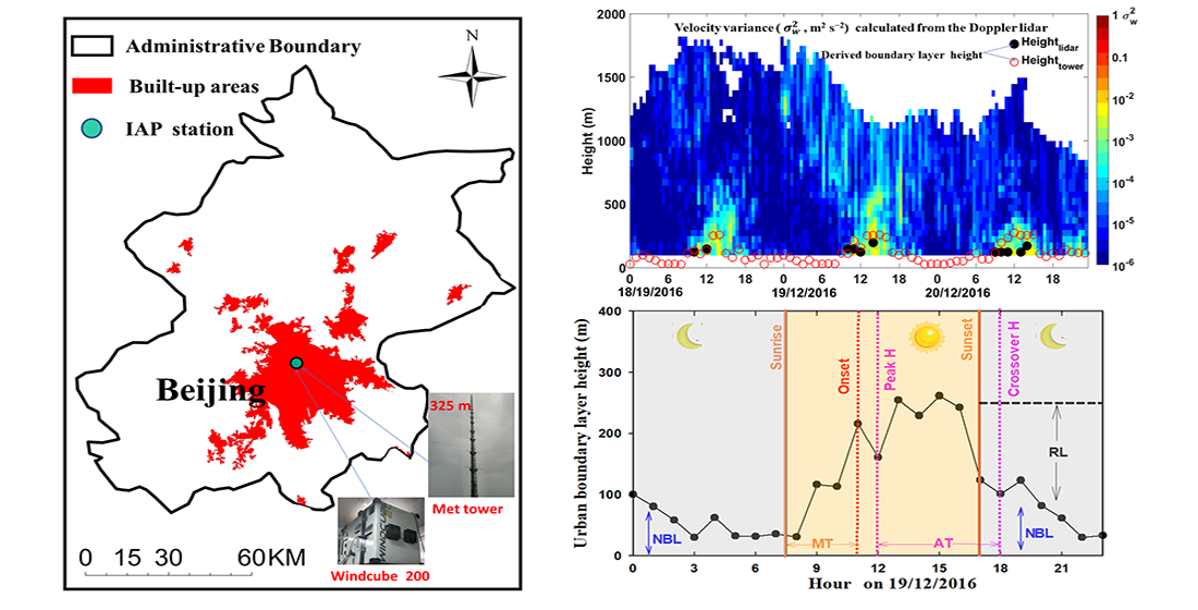
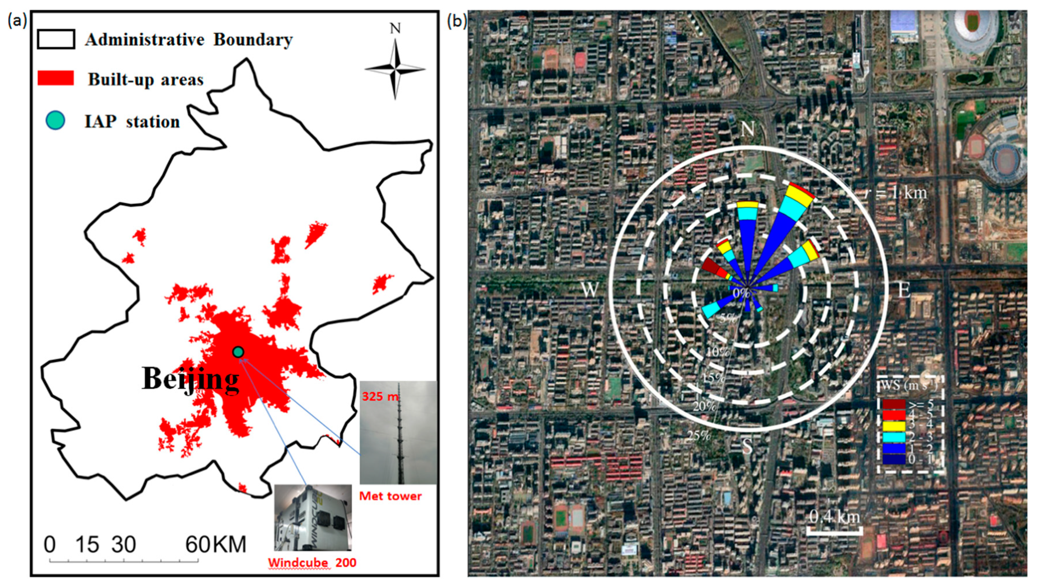
2.1. Experimental Sites and Instrumentation
2.2. Data Processing
2.3. Methods
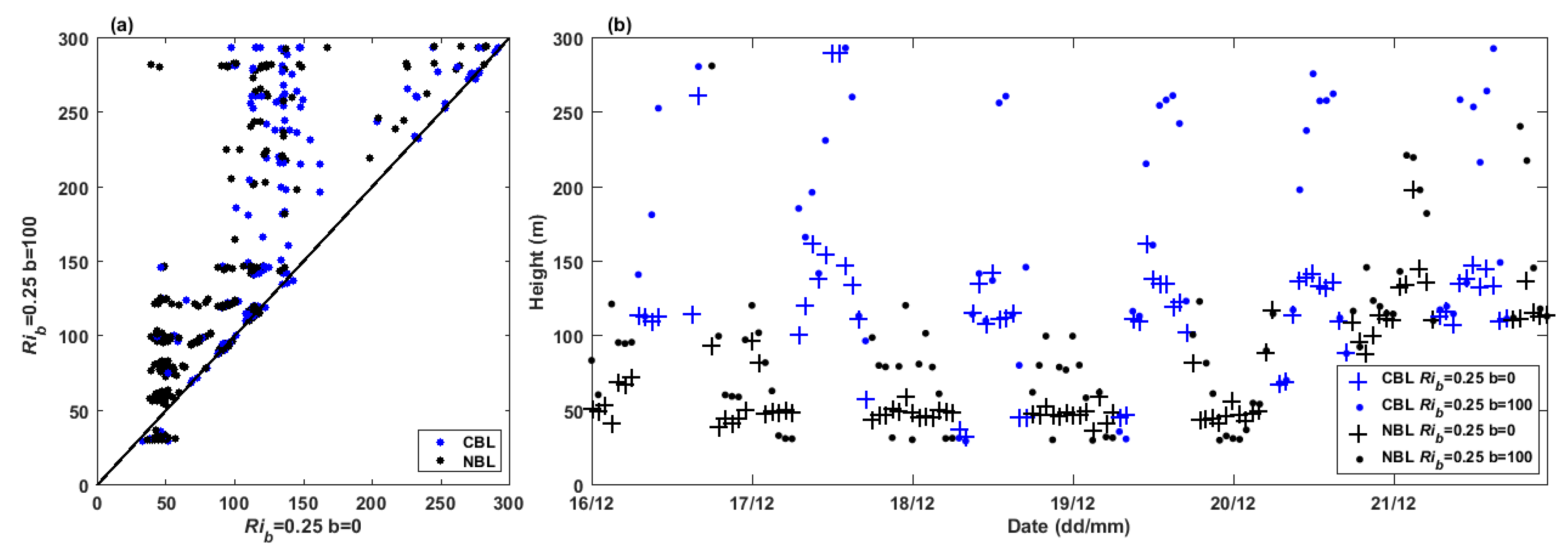
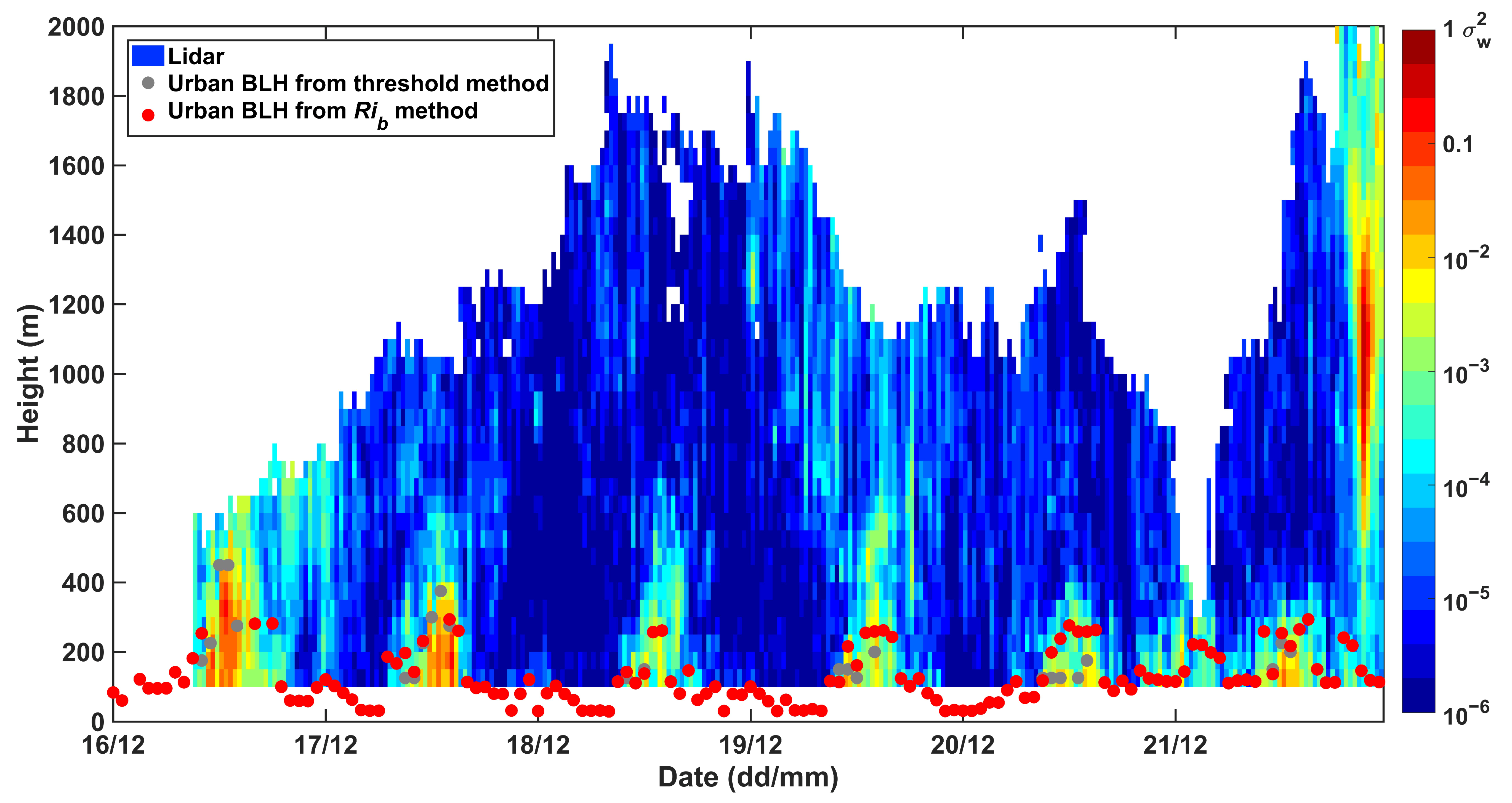
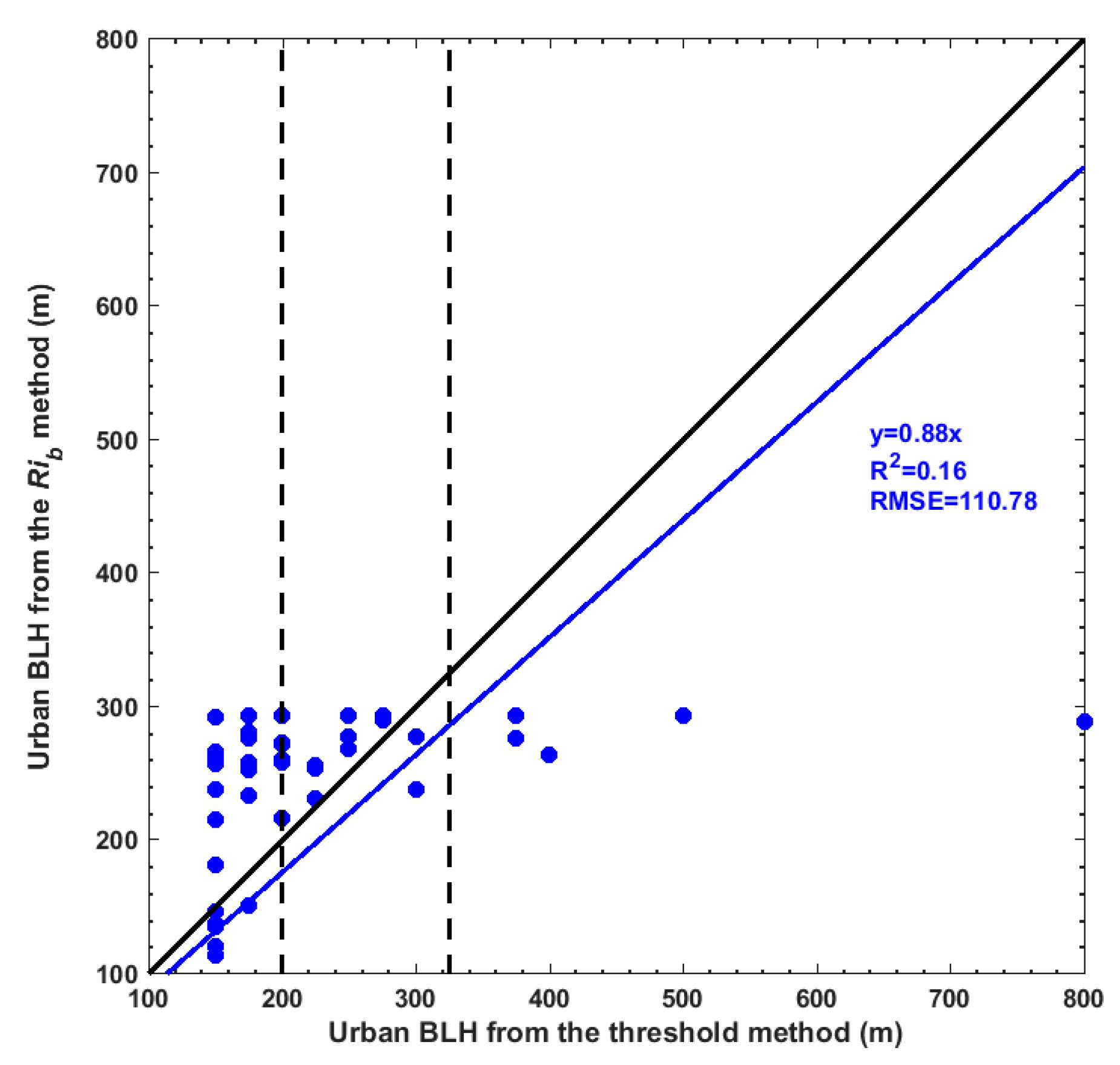
2.3.1. Estimation of Urban BLH
2.3.2. Calculation of Heat Flux
3. Results
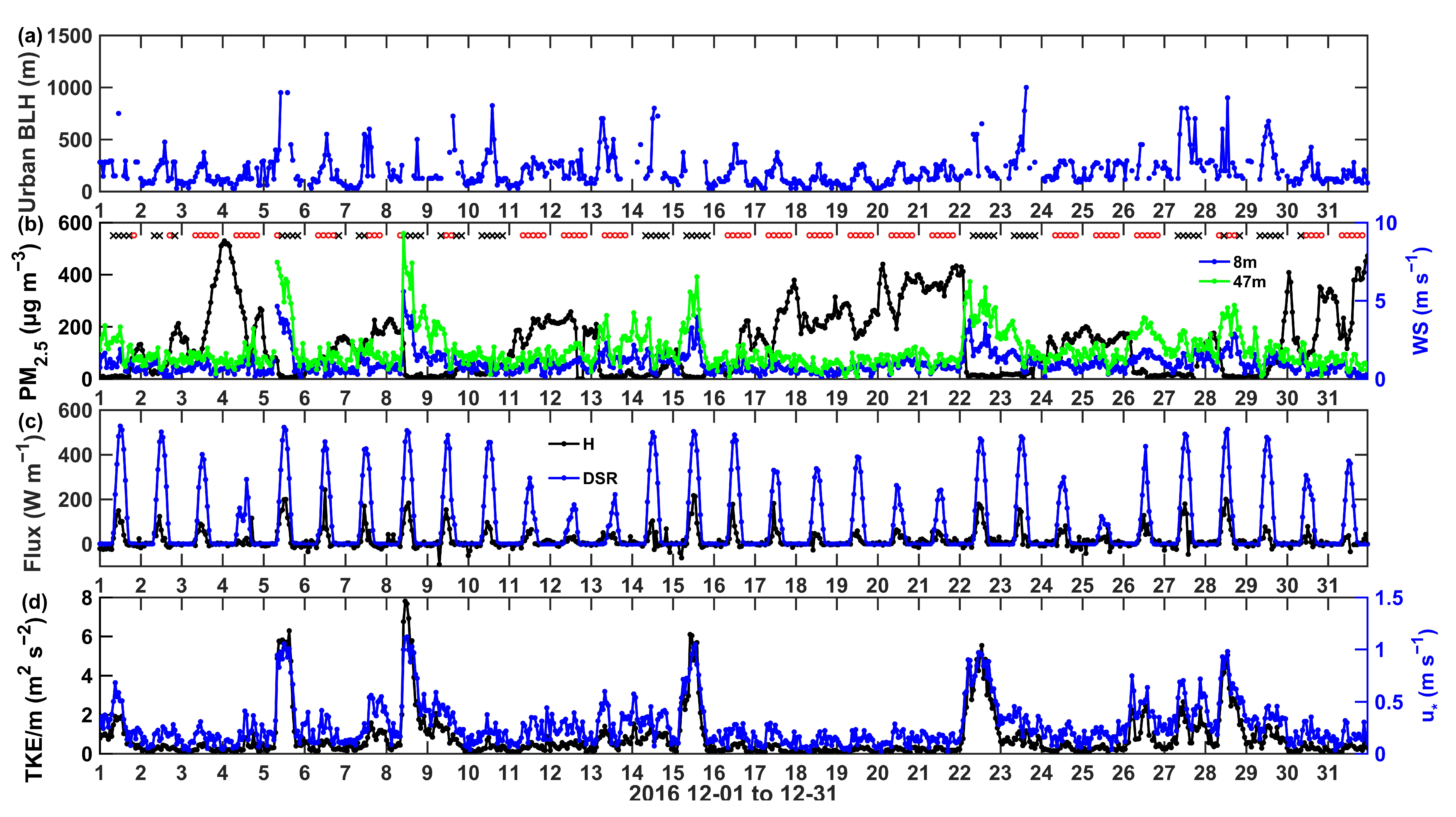
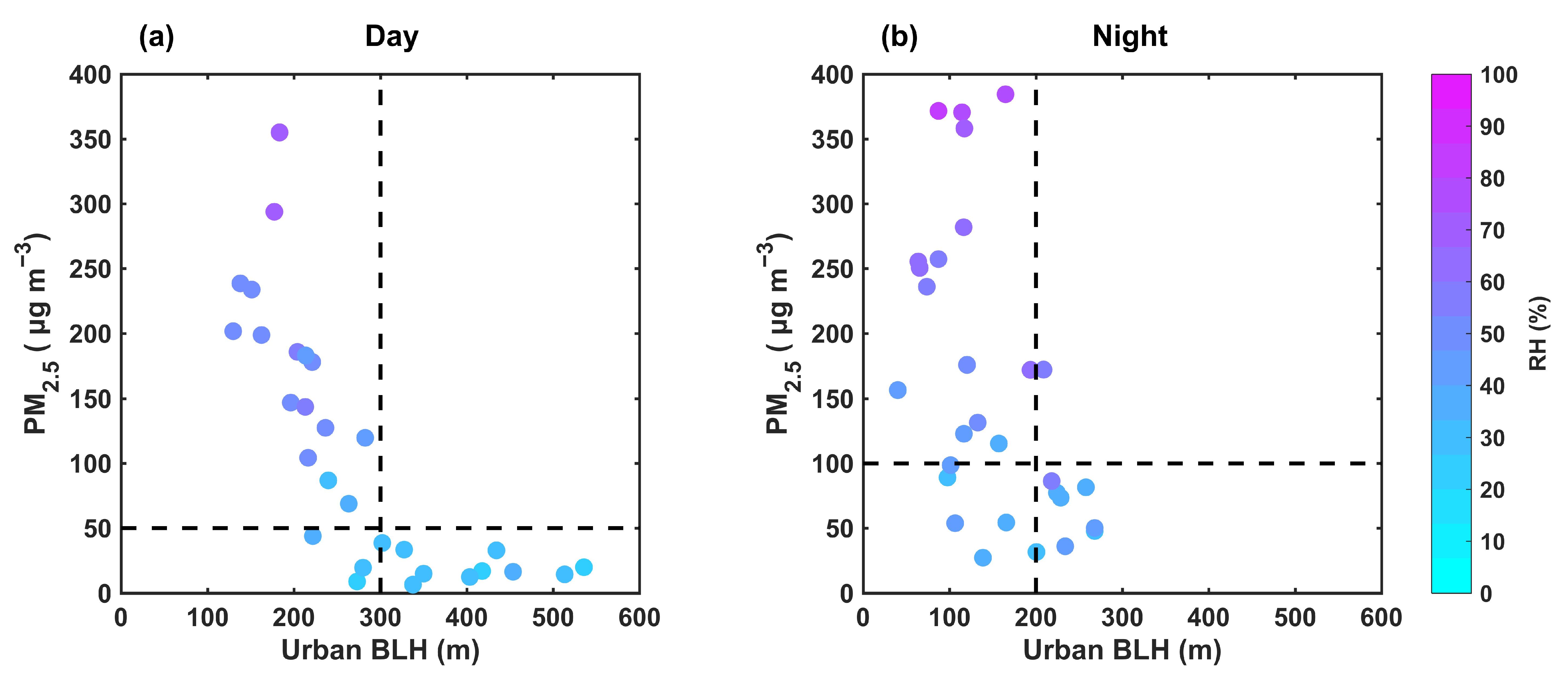
3.1. Urban BLH
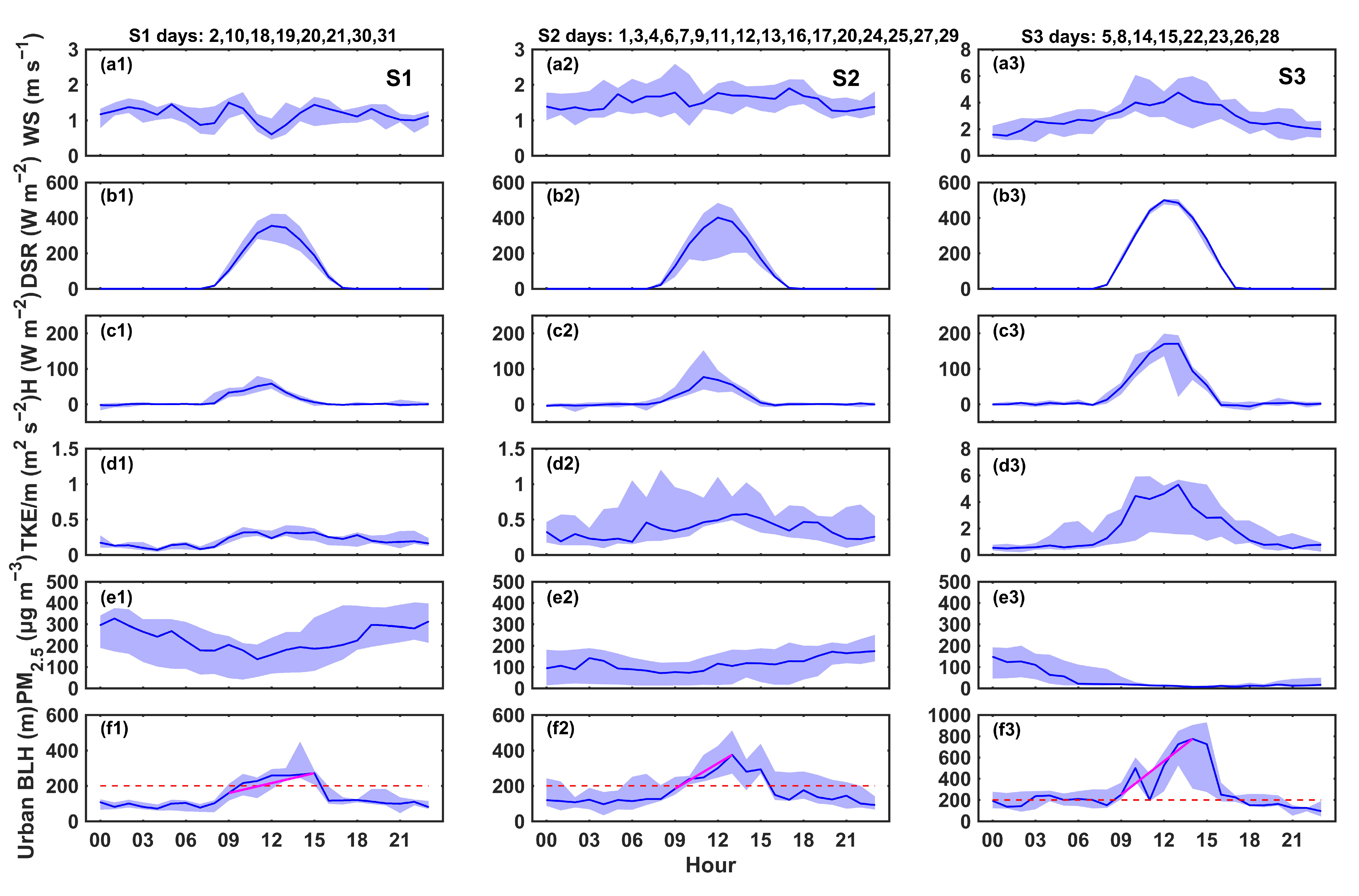
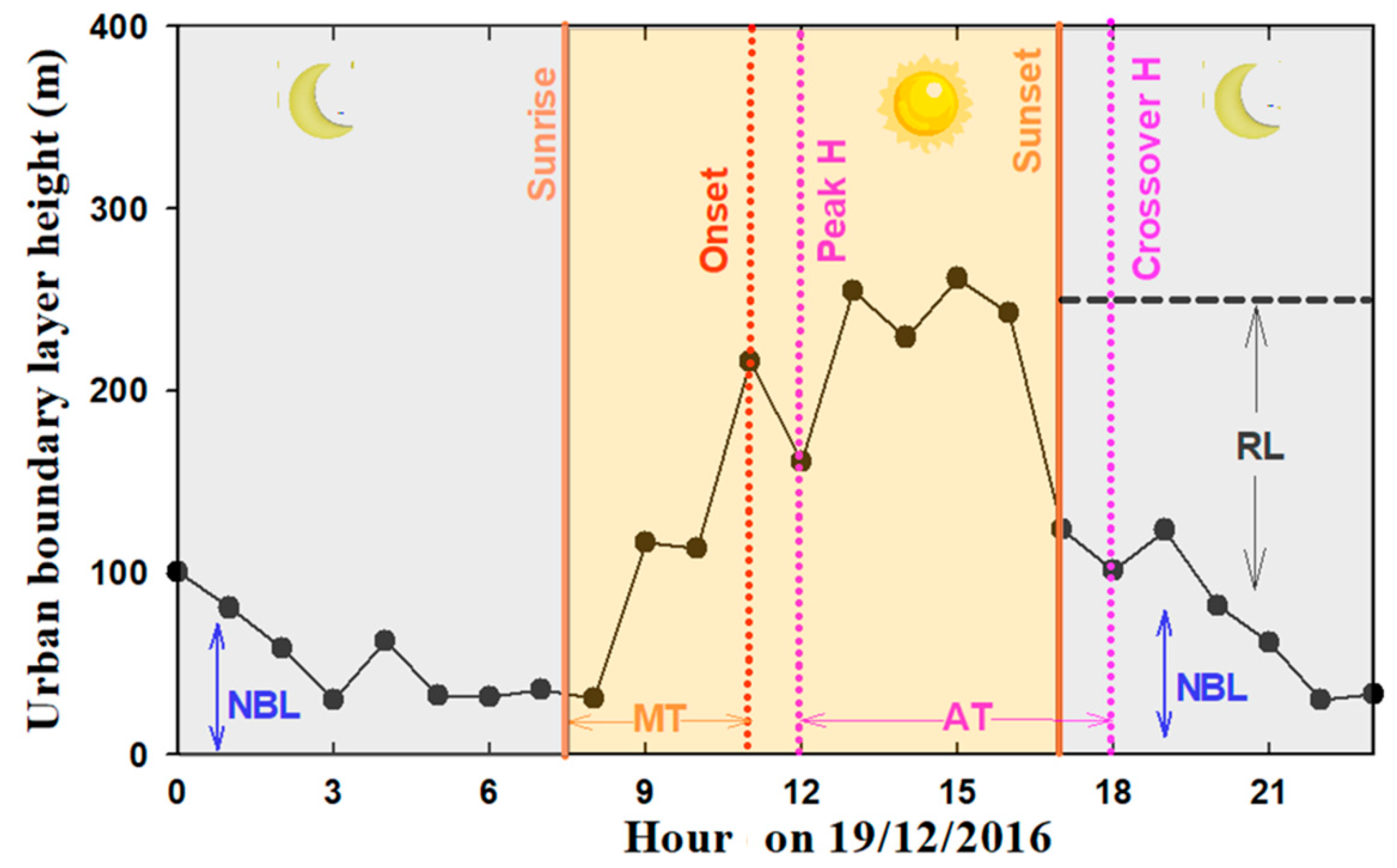
3.2. Diurnal Development of the Urban Boundary Layer
3.3. Morning and Afternoon Transitions of the Urban Boundary Layer
3.3.1. Durations
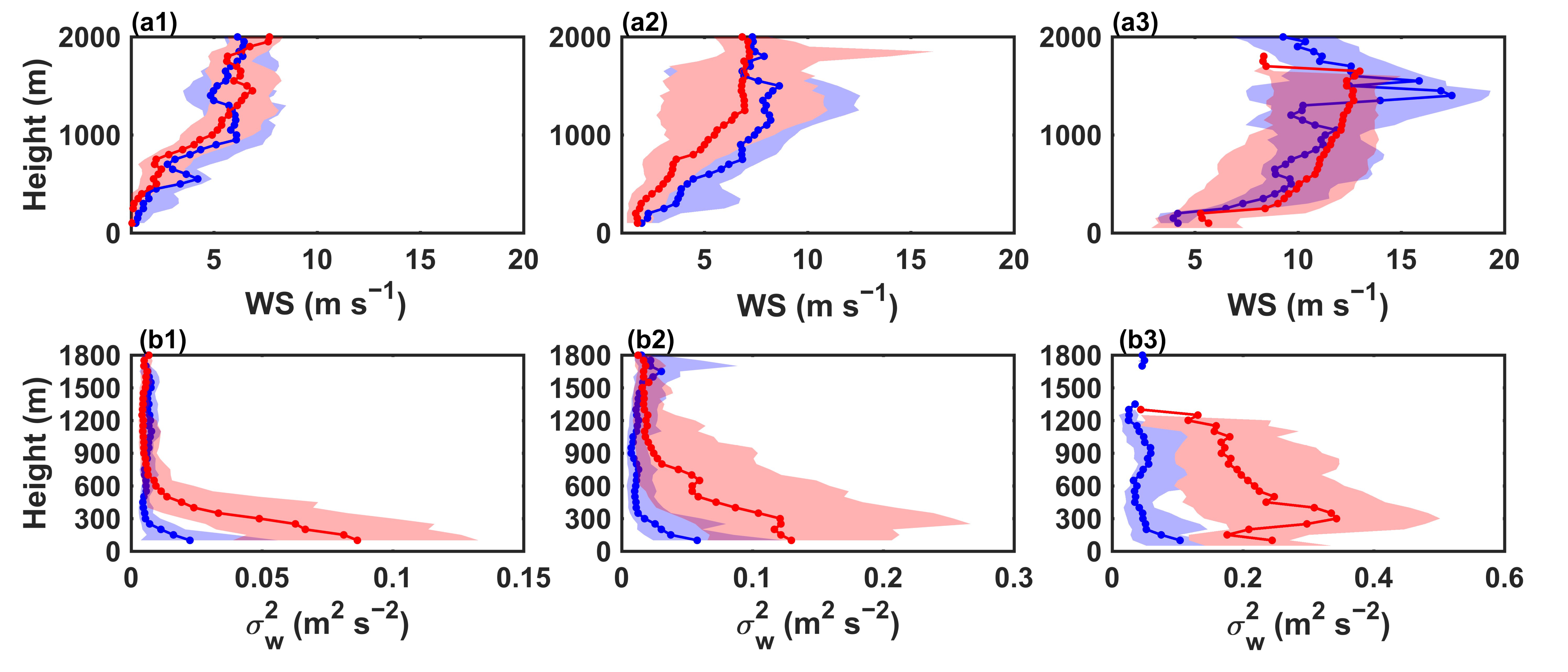
3.3.2. WS and Vertical Variance Profiles
4. Discussions
5. Conclusions
Supplementary Materials
Author Contributions
Funding
Acknowledgments
Conflicts of Interest
References
- Collier, C.; Davies, F.; Bozier, K.; Holt, A.; Middleton, D.; Pearson, G.; Siemen, S.; Willetts, D.; Upton, G.; Young, R. Dual Doppler Lidar Measurements for Improving Dispersion Models. B. Am. Meteorol. Soc. 2005, 86, 825–838. [Google Scholar] [CrossRef]
- White, J.M.; Bowers, J.F.; Hanna, S.R.; Lundquist, J.K. Importance of Using Observations of Mixing Depths in order to Avoid Large Prediction Errors by a Transport and Dispersion Model. J. Atmos. Ocean. Tech. 2009, 26, 22–32. [Google Scholar] [CrossRef]
- Schween, J.H.; Hirsikko, A.; Löhnert, U.; Crewell, S. Mixing-layer height retrieval with ceilometer and Doppler lidar: From case studies to long-term assessment. Atmos. Meas. Tech. 2014, 7, 3685–3704. [Google Scholar] [CrossRef] [Green Version]
- Jia, W.X.; Zhang, X.Y. The role of the planetary boundary layer parameterization schemes on the meteorological and aerosol pollution simulations: A review. Atmos. Res. 2020, 239, 104890. [Google Scholar] [CrossRef]
- Schäfer, K.; Emeis, S.; Hoffmann, H.; Jahn, C. Influence of mixing layer height upon air pollution in urban and sub-urban areas. Meteorol. Z. 2006, 15, 647–658. [Google Scholar] [CrossRef] [Green Version]
- Salamanca, F.; Martilli, A.; Tewari, M.; Chen, F. A study of the urban boundary layer using different urban parameterizations and high-resolution urban canopy parameters with WRF. J. Appl. Meteorol. Clim. 2001, 50, 1107–1128. [Google Scholar] [CrossRef]
- Miao, S.G.; Chen, F.; LeMone, M.A.; Tewari, M.; Li, Q.; Wang, Y. An observational and modeling study of characteristics of urban heat island and boundary layer structures in Beijing. J. Appl. Meteorol. Clim. 2009, 48, 484–501. [Google Scholar] [CrossRef]
- Lothon, M.; Lohou, F.; Pino, D.; Couvreux, F.; Pardyjak, E.R.; Reuder, J.; Vilà-Guerau de Arellano, J.; Durand, P.; Hartogensis, O.; Legain, D.; et al. The BLLAST field experiment: Boundary-Layer Late Afternoon and Sunset Turbulence. Atmos. Chem. Phys. 2014, 14, 10931–10960. [Google Scholar] [CrossRef] [Green Version]
- Piringer, M.; Joffre, S.; Baklanov, A.; Christen, A.; Deserti, M.; Ridder, K.; Emeis, S.; Mestayer, P.; Tombrou, M.; Middleton, D.; et al. The surface energy balance and the mixing height in urban areas—Activities and recommendations of COST-Action 715. Boundary-Layer Meteorol. 2007, 124, 3–24. [Google Scholar] [CrossRef]
- Liu, B.M.; Ma, Y.Y.; Gong, W.; Zhang, M.; Yang, J. Determination of boundary layer top on the basis of the characteristics of atmospheric particles. Atmos. Environ. 2018, 178, 140–147. [Google Scholar] [CrossRef]
- Shi, Y.; Hu, F.; Fan, G.Q.; Zhang, Z. Multiple technical observations of the atmospheric boundary layer structure of a red-alert haze episode in Beijing. Atmos. Meas. Tech. 2019, 12, 4887–4901. [Google Scholar] [CrossRef] [Green Version]
- Banta, R.M.; Senff, C.J.; White, A.B.; Trainer, M.; McNider, R.T.; Valente, R.J.; Mayor, S.D.; Alvarez, R.J.; Hardesty, R.M.; Parrish, D.; et al. Daytime buildup and nighttime transport of urban ozone in the boundary layer during a stagnation episode. J. Geophys. Res. Atmos. 1998, 103, 22519–22544. [Google Scholar] [CrossRef]
- Banta, R.M.; White, A.B. Mixing-height differences between land use types: Dependence on wind speed. J. Geophys. Res. Atmos. 2003, 108, D10. [Google Scholar] [CrossRef]
- Lolli, S.; Paolo, D. Principal component analysis approach to evaluate instrument performances in developing a cost-effective reliable instrument network for atmospheric measurements. J. Atmos. Ocean. 2015, 32, 1642–1649. [Google Scholar] [CrossRef]
- Kotthaus, S.; Halios, C.H.; Barlow, J.F.; Grimmond, C.S.B. Volume for pollution dispersion: London’s atmospheric boundary layer during ClearfLo observed with two ground-based lidar types. Atmos. Environ. 2018, 190, 401–414. [Google Scholar] [CrossRef] [Green Version]
- Yin, J.; Gao, Y.C.; Hong, J.; Gao, Z.Q.; Li, Y.; Li, X.; Zhu, B. Surface meteorological conditions and boundary layer height variations during air pollution episode in Nanjing, China. J. Geophys. Res. Atmos. 2018, 124, 3350–3364. [Google Scholar] [CrossRef]
- Seibert, P.; Beyrich, F.; Gryning, S.E.; Joffre, S.; Rasmussen, A.; Tercier, P. Review and intercomparison of operational methods for the determination of the mixing height. Atmos. Environ. 2000, 34, 1001–1027. [Google Scholar] [CrossRef]
- Contini, D.; Cava, D.; Martano, P.; Donateo, A.; Grasso, F.M. Comparison of indirect methods for the estimation of boundary layer height over fat-terrain in a coast site. Meteorol. Z. 2009, 18, 309–320. [Google Scholar] [CrossRef]
- Lolli, S.; Delaval, A.; Loth, C.; Garnier, A.; Flamant, P.H. 0.355-micrometer direct detection wind lidar under testing during a field campaign in consideration of ESA’s ADM-Aeolus mission. Atmos. Meas. Tech. 2013, 6, 3349–3358. [Google Scholar] [CrossRef] [Green Version]
- Ciofini, M.; Lapucci, A.; Lolli, S. Diffractive optical components for high power laser beam sampling. J. Opt. A-Pure Appl. Op. 2003, 5, 186–191. [Google Scholar] [CrossRef]
- Barlow, J.F.; Dunbar, T.M.; Nemitz, E.G.; Wood, C.R.; Gallagher, M.W.; Davies, F.; O’Connor, E.; Harrison, R.M. Boundary layer dynamics over London, UK, as observed using Doppler lidar during REPARTEE-II. Atmos. Chem. Phys. 2011, 11, 2111–2125. [Google Scholar] [CrossRef] [Green Version]
- Park, S.; Kim, S.W.; Park, M.S.; Song, C.K. Measurement of Planetary Boundary Layer Winds with Scanning Doppler Lidar. Remote Sens. 2018, 10, 1261. [Google Scholar] [CrossRef] [Green Version]
- Yang, Y.J.; Yim, S.H.L.; Haywood, J.; Osborne, M.; Chan, J.C.S.; Zeng, Z.L.; Cheng, J.C.H. Characteristics of Heavy Particulate Matter Pollution Events Over Hong Kong and Their Relationships With Vertical Wind Profiles Using High-Time-Resolution Doppler Lidar Measurements. J. Geophys. Res. Atmos. 2019, 124, 9609–9623. [Google Scholar] [CrossRef] [Green Version]
- Steve, H.L. Development of a 3D Real-Time Atmospheric Monitoring System (3DREAMS) Using Doppler LiDARs and Applications for Long-Term Analysis and Hot-and-Polluted Episodes. Remote Sens. 2020, 12, 1036. [Google Scholar]
- Huang, T.; Yim, S.-L.; Yang, Y.; Lee, O.-M.; Lam, D.-Y.; Cheng, J.-H.; Guo, J. Observation of Turbulent Mixing Characteristics in the Typical Daytime Cloud-Topped Boundary Layer over Hong Kong in 2019. Remote Sens. 2020, 12, 1533. [Google Scholar] [CrossRef]
- Liu, Z.L.; Barlow, J.F.; Chan, P.-W.; Fung, J.H.; Li, Y.G.; Ren, C.; Mak, H.W.L.; Ng, E. A Review of Progress and Applications of Pulsed Doppler Wind LiDARs. Remote Sens. 2019, 11, 2522. [Google Scholar] [CrossRef] [Green Version]
- Huang, M.; Gao, Z.Q.; Miao, S.G.; Chen, F.; LeMone, M.A.; Li, J.; Hu, F.; Wang, L.L. Estimate of boundary-layer depth over Beijing, China, using Doppler Lidar data during SURF-2015. Boundary-Layer Meteorol. 2017, 162, 503–522. [Google Scholar] [CrossRef] [Green Version]
- LeMone, M.A.; Tewari, M.; Chen, F.; Dudhia, J. Objectively Determined Fair-Weather NBL Features in ARW-WRF and Their Comparison to CASES-97 Observations. Mon. Weather Rev. 2014, 142, 2709–2732. [Google Scholar] [CrossRef] [Green Version]
- Wang, L.L.; Liu, J.K.; Gao, Z.Q.; Li, Y.B.; Huang, M.; Fan, S.H.; Zhang, X.Y.; Yang, Y.J.; Miao, S.G.; Zou, H.; et al. Vertical observations of the atmospheric boundary layer structure over Beijing urban area during air pollution episodes. Atmos. Chem. Phys. 2019, 19, 6949–6967. [Google Scholar]
- Li, J.; Sun, J.L.; Zhou, M.Y.; Cheng, Z.G.; Li, Q.C.; Cao, X.Y.; Zhang, J.J. Observational analyses of dramatic developments of a severe air pollution event in the Beijing area. Atmos. Chem. Phys. 2018, 18, 3919–3935. [Google Scholar] [CrossRef] [Green Version]
- Zhong, J.T.; Zhang, X.Y.; Dong, Y.S.; Wang, Y.Q.; Liu, C.; Wang, J.Z.; Zhang, Y.M.; Che, H.C. Feedback effects of boundary-layer meteorological factors on cumulative explosive growth of PM2.5 during winter heavy pollution episodes in Beijing from 2013 to 2016. Atmos. Chem. Phys. 2018, 18, 247–258. [Google Scholar] [CrossRef] [Green Version]
- Pournazeri, S.; Venkatram, A.; Princevac, M.; Tan, S.; Schulte, N. Estimating the height of the nocturnal urban boundary layer for dispersion applications. Atmos. Environ. 2012, 54, 611–623. [Google Scholar] [CrossRef]
- Liu, J.K.; Gao, Z.Q.; Wang, L.L.; Li, Y.B.; Gao, C.Y. The impact of urbanization on wind speed and surface aerodynamic characteristics in Beijing during 1991–2011. Meteorol. Atmos. Phys. 2017, 130, 311–324. [Google Scholar] [CrossRef]
- Wang, L.L.; Fan, S.H.; Hu, F.; Miao, S.G.; Yang, A.Q.; Li, Y.B.; Liu, J.J.; Liu, C.W.; Chen, S.S.; Ho, H.C.; et al. Vertical Gradient Variations in Radiation Budget and Heat Fluxes in the Urban Boundary Layer: A Comparison Study Between Polluted and Clean Air Episodes in Beijing During Winter. J. Geophys. Res. Atmos. 2020, 125, e2020JD032478. [Google Scholar] [CrossRef]
- Detto, M.; Katul, G.G. Simplified expressions for adjusting higher-order turbulent statistics obtained from open path gas analyzers. Boundary-Layer Meteorol. 2007, 122, 205–216. [Google Scholar] [CrossRef]
- Wilczak, J.M.; Oncley, S.P.; Stage, S.A. Sonic anemometer tilt correction algorithms. Boundary-Layer Meteorol. 2001, 99, 127–150. [Google Scholar] [CrossRef]
- Wang, L.L.; Li, D.; Gao, Z.Q.; Sun, T.; Guo, X.F.; Bou-Zeid, E. Turbulent transport of momentum and scalars above an urban canopy. Boundary-Layer Meteorol. 2014, 150, 485–511. [Google Scholar] [CrossRef]
- Seidel, D.J.; Zhang, Y.H.; Beljaars, A.; Golaz, J.-C.; Jacobson, A.R.; Medeiros, B. Climatology of the planetary boundary layer over the continental United States and Europe. J. Geophys. Res. Atmos. 2012, 117, D17106. [Google Scholar] [CrossRef]
- Wang, D.X.; Stachlewska, I.S.; Song, X.Q.; Heese, B.; Nemuc, A. Variability of the Boundary Layer Over an Urban Continental Site Based on 10 Years of Active Remote Sensing Observations in Warsaw. Remote Sens. 2020, 12, 340. [Google Scholar] [CrossRef] [Green Version]
- Vogelezang, D.H.P.; Holtslag, A.A.M. Evaluation and model impacts of alternative boundary-layer height formulation. Boundary Layer Meteorol. 1996, 81, 245–269. [Google Scholar] [CrossRef]
- Zhang, Y.J.; Gao, Z.Q.; Li, D.; Li, Y.B.; Zhang, N.; Zhao, X.; Chen, J. On the computation of planetary boundary-layer height using the bulk Richardson number method. Geosci. Model Dev. 2014, 7, 2599–2611. [Google Scholar] [CrossRef] [Green Version]
- Guo, J.P.; Miao, Y.C.; Zhang, Y.; Liu, H.; Li, Z.Q.; Zhang, W.C.; He, J.; Lou, M.Y.; Yan, Y.; Bian, L.G.; et al. The climatology of planetary boundary layer height in China derived from radiosonde and reanalysis data. Atmos. Chem. Phys. 2016, 16, 13309–13319. [Google Scholar] [CrossRef] [Green Version]
- Zhang, Y.H.; Li, S.Y. Climatological characteristics of planetary boundary layer height over Japan. Int. J. Climatol. 2019, 39, 4015–4028. [Google Scholar] [CrossRef]
- Zhang, Y.J.; Sun, K.; Gao, Z.Q.; Pan, Z.T.; Shook, M.; Li, D. Diurnal climatology of planetary boundary layer height over the contiguous United States derived from AMDAR and reanalysis data. J. Geophys. Res. Atmos. 2020. (under review). [Google Scholar] [CrossRef]
- Angevine, W.M.; Klein, B.H.; Bosveld, F.C. Observations of the morning transition of the convective boundary layer. Boundary-Layer Meteorol. 2001, 101, 209–227. [Google Scholar] [CrossRef]
- Chu, Y.Q.; Li, J.; Li, C.C.; Tan, W.S.; Su, T.N.; Li, J. Seasonal and diurnal variability of planetary boundary layer height in Beijing: Intercomparison between MPL and WRF results. Atmos. Res. 2019, 227, 1–23. [Google Scholar] [CrossRef]
- Wang, L.L.; Wang, H.; Liu, J.K.; Gao, Z.Q.; Yang, Y.J.; Zhang, X.Y.; Li, Y.B.; Huang, M. Impacts of the near-surface urban boundary layer structure on PM2.5 concentrations in Beijing during winter. Sci. Total Environ. 2019, 669, 493–504. [Google Scholar] [CrossRef]
- Stull, R.B. An Introduction to Boundary Layer Meteorology; Kuwer Academic Publishers: Dordrecht, The Netherlands, 1988; pp. 2–189. [Google Scholar]
- Tucker, S.C.; Senff, C.J.; Weickmann, A.M.; Brewer, W.A.; Banta, R.M.; Sandberg, S.P.; Law, D.C.; Hardesty, R.M. Doppler lidar estimation of mixing height using turbulence, shear, and aerosol profiles. J. Atmos. Ocean. Technol. 2009, 26, 673–688. [Google Scholar] [CrossRef]
- Harvey, N.J.; Hogan, R.J.; Dacre, H.F. A method to diagnose boundary-layer type using Doppler lidar. Q. J. Roy. Meteor. Soc. 2013, 139, 1681–1693. [Google Scholar] [CrossRef]
- Angevine, W.M.; Edwards, J.M.; Lothon, M.; LeMone, M.A.; Osborne, S.R. Transition Periods in the Diurnally-Varying Atmospheric Boundary Layer Over Land. Boundary-Layer Meteorol. 2020, 53, 631. [Google Scholar]
- Kotthaus, S.; Grimmond, C.S.B. Atmospheric boundary-layer characteristics from ceilometer measurements. Part 1: A new method to track mixed layer height and classify clouds. Q. J. Roy. Meteor. Soc. 2018, 144, 1525–1538. [Google Scholar] [CrossRef] [Green Version]
- Tang, G.Q.; Zhang, J.Q.; Zhu, X.W.; Song, T.; Munkel, C.; Hu, B.; Schafer, K.; Liu, Z.R.; Zhang, J.K.; Wang, L.L.; et al. Mixing layer height and its implications for air pollution over Beijing, China. Atmos. Chem. Phys. 2016, 16, 2459–2475. [Google Scholar] [CrossRef] [Green Version]
- Miao, Y.C.; Guo, J.P.; Liu, S.H.; Zhao, C.; Li, X.L.; Zhang, G.; Wei, W.; Ma, Y.J. Impacts of synoptic condition and planetary boundary layer structure on the trans-boundary aerosol transport from Beijing-Tianjin-Hebei region to northeast China. Atmos. Environ. 2018, 181, 1–11. [Google Scholar] [CrossRef]
- Sun, Y.L.; Jiang, Q.; Wang, Z.F.; Fu, P.Q.; Li, J.; Yang, T.; Yin, Y. Investigation of the sources and evolution processes of severe haze pollution in Beijing in January 2013. J. Geophys. Res. Atmos. 2014, 119, 4380–4398. [Google Scholar] [CrossRef]
- Li, Z.Q.; Guo, J.P.; Ding, A.J.; Liao, H.; Liu, J.J.; Sun, Y.L.; Wang, T.J.; Xue, H.W.; Zhang, H.S.; Zhu, B. Aerosol and boundary-layer interactions and impact on air quality. Natl. Sci. Rev. 2017, 4, 810–833. [Google Scholar] [CrossRef]
- Tan, S.C.; Zhang, X.; Wang, H.; Chen, B.; Shi, G.Y.; Shi, C. Comparisons of cloud detection among four satellite sensors on severe haze days in eastern china. Atmos. Ocean. Sci. Lett. 2018, 11, 86–93. [Google Scholar] [CrossRef] [Green Version]
- Halios, C.H.; Barlow, J.F. Observations of the Morning Development of the Urban Boundary Layer over London, UK, Taken During the ACTUAL Project. Boundary-Layer Meteorol. 2018, 166, 395–422. [Google Scholar] [CrossRef]
- Price, J. On the formation and development of radiation fog: An observational study. Boundary-Layer Meteorol. 2019, 172, 167–197. [Google Scholar] [CrossRef]
- Bange, J.; Spiess, T.; van den Kroonenberg, A. Characteristics of the early-morning shallow convective boundary layer from Helipod Flights during STINHO-2. Theor. Appl. Climatol. 2007, 90, 113–126. [Google Scholar] [CrossRef]
- Pal, S.; Haeffelin, M.; Batchvarova, E. Exploring a geophysical process-based attribution technique for the determination of the atmospheric boundary layer depth using aerosol lidar and near-surface meteorological measurements. J. Geophys. Res. Atmos. 2013, 118, 9277–9295. [Google Scholar] [CrossRef]
- Nadeau, D.F.; Pardyjak, E.; Higgins, C.W.; Fernando, H.J.S.; Parlange, M.B. A simple model for the afternoon and early evening decay of convective turbulence over different land surfaces. Boundary-Layer Meteorol. 2011, 141, 301–324. [Google Scholar] [CrossRef] [Green Version]
- Beare, R.J. The Role of Shear in the Morning Transition Boundary Layer. Boundary-Layer Meteorol. 2008, 129, 395–410. [Google Scholar] [CrossRef]
- Barbaro, E.; de Arellano, J.V.-G.; Ouwersloot, H.G.; Schröter, J.S.; Donovan, D.P.; Krol, M.C. Aerosols in the convective boundary layer: Shortwave radiation effects on the coupled land-atmosphere system. J. Geophys. Res. Atmos. 2014, 119, 5845–5863. [Google Scholar] [CrossRef]
- Driedonks, A.G.M. Models and observations of the growth of the atmospheric boundary layer. Boundary-Layer Meteorol. 1982, 23, 283–306. [Google Scholar] [CrossRef]
- Donateo, A.; Contini, D.; Belosi, F.; Gambaro, A.; Santachiara, G.; Cesari, D.; Prodi, F. Charaterisation of PM2.5 concentrations and turbulent fluxes on an island of Venice lagoon using high temporal resolution measurements. Meteorol. Z. 2012, 21, 385–398. [Google Scholar] [CrossRef] [Green Version]
- Zhang, X.Y.; Sun, J.Y.; Wang, Y.Q.; Li, W.J.; Zhang, Q.; Wang, W.G.; Quan, J.N.; Cao, G.L.; Wang, J.Z.; Yang, Y.Q.; et al. Factors contributing to haze and fog in china. Chin. Sci. Bull. 2013, 58, 1178. [Google Scholar]
- Han, S.Q.; Hao, T.Y.; Zhang, Y.F.; Liu, J.L.; Li, P.Y.; Cai, Z.; Zhang, M.; Wang, Q.L.; Zhang, H. Vertical observation and analysis on rapid formation and evolutionary mechanisms of a prolonged haze episode over central-eastern China. Sci. Total Environ. 2018, 616–617, 135–146. [Google Scholar] [CrossRef]
- Salmond, J.A.; McKendry, I.G. A review of turbulence in the very stable nocturnal boundary layer and its implications for air quality. Prog. Phys. Geog. 2015, 29, 171–188. [Google Scholar] [CrossRef] [Green Version]
- Miao, Y.C.; Guo, J.P.; Liu, S.H.; Wei, W.; Zhang, G.; Lin, Y.L.; Zhai, P.M. The climatology of low-level jet in Beijing and Guangzhou, China. J. Geophys. Res. Atmos. 2018, 123, 2816–2830. [Google Scholar] [CrossRef]
- Banta, R.M.; Newsom, R.K.; Lundquist, J.K.; Pichugina, Y.L.; Coulter, R.L.; Mahrt, L. Nocturnal low-level jet characteristics over Kansas during cases-99. Boundary-Layer Meteorol. 2002, 105, 221–252. [Google Scholar] [CrossRef]
- Hu, X.M.; Ma, Z.Q.; Lin, W.L.; Zhang, H.L.; Hu, J.L.; Wang, Y.; Xu, X.B.; Fuentes, J.D.; Xue, M. Impact of the Loess Plateau on the atmospheric boundary layer structure and air quality in the North China Plain: A case study. Sci. Total Environ. 2014, 499, 228–237. [Google Scholar] [CrossRef]
- Chen, Y.; An, J.L.; Sun, Y.L.; Wang, X.Q.; Qu, Y.; Zhang, J.W.; Wang, Z.F.; Duan, J. Nocturnal low-level winds and their impacts on particulate matter over the Beijing area. Adv. Atmos. Sci. 2018, 35, 1455–1468. [Google Scholar] [CrossRef]
- Petäjä, T.; Järvi, L.; Kerminen, V.M.; Ding, A.J.; Sun, J.N.; Nie, W.; Kujansuu, J.; Virkkula, A.; Yang, X.Q.; Fu, C.B.; et al. Enhanced air pollution via aerosol-boundary layer feedback in China. Sci. Rep. 2016, 6, 1–6. [Google Scholar] [CrossRef] [Green Version]
- Zhong, J.T.; Zhang, X.Y.; Wang, Y.Q.; Wang, J.Z.; Shen, X.J.; Zhang, H.S.; Wang, T.J.; Xie, Z.Q.; Liu, C.; Zhang, H.D.; et al. The two-way feedback mechanism between unfavorable meteorological conditions and cumulative aerosol pollution in various haze regions of China. Atmos. Chem. Phys. 2019, 19, 3287–3306. [Google Scholar] [CrossRef] [Green Version]
- Yang, Y.J.; Zheng, Z.F.; Yim, S.H.L.; Roth, M.; Ren, G.; Gao, Z.Q.; Wang, T.; Li, Q.; Shi, C.; Ning, G.; et al. PM2.5 pollution modulates wintertime Urban-Heat-Island intensity in the Beijing-Tianjin-Hebei megalopolis, China. Geophys. Res. Lett. 2020, 47, e2019GL084288. [Google Scholar] [CrossRef] [Green Version]
- Ding, A.J.; Fu, C.B.; Yang, X.Q.; Sun, J.N.; Petäjä, T.; Kerminen, V.M.; Wang, T.; Xie, Y.; Herrmann, E.; Zheng, L.F.; et al. Intense atmospheric pollution modifies weather: A case of mixed biomass burning with fossil fuel combustion pollution in eastern China. Atmos. Chem. Phys. 2013, 13, 10545–10554. [Google Scholar] [CrossRef] [Green Version]
- Lolli, S.; Khor, W.Y.; Matjafri, M.Z.; Lim, H.S. Monsoon season quantitative assessment of biomass burning clear-sky aerosol radiative effect at surface by ground-based lidar observations in Pulau Pinang, Malaysia in 2014. Remote Sens. 2019, 11, 2660. [Google Scholar] [CrossRef] [Green Version]


Publisher’s Note: MDPI stays neutral with regard to jurisdictional claims in published maps and institutional affiliations. |
© 2020 by the authors. Licensee MDPI, Basel, Switzerland. This article is an open access article distributed under the terms and conditions of the Creative Commons Attribution (CC BY) license (http://creativecommons.org/licenses/by/4.0/).
Share and Cite
Yang, Y.; Fan, S.; Wang, L.; Gao, Z.; Zhang, Y.; Zou, H.; Miao, S.; Li, Y.; Huang, M.; Yim, S.H.L.; et al. Diurnal Evolution of the Wintertime Boundary Layer in Urban Beijing, China: Insights from Doppler Lidar and a 325-m Meteorological Tower. Remote Sens. 2020, 12, 3935. https://doi.org/10.3390/rs12233935
Yang Y, Fan S, Wang L, Gao Z, Zhang Y, Zou H, Miao S, Li Y, Huang M, Yim SHL, et al. Diurnal Evolution of the Wintertime Boundary Layer in Urban Beijing, China: Insights from Doppler Lidar and a 325-m Meteorological Tower. Remote Sensing. 2020; 12(23):3935. https://doi.org/10.3390/rs12233935
Chicago/Turabian StyleYang, Yuanjian, Sihui Fan, Linlin Wang, Zhiqiu Gao, Yuanjie Zhang, Han Zou, Shiguang Miao, Yubin Li, Meng Huang, Steve Hung Lam Yim, and et al. 2020. "Diurnal Evolution of the Wintertime Boundary Layer in Urban Beijing, China: Insights from Doppler Lidar and a 325-m Meteorological Tower" Remote Sensing 12, no. 23: 3935. https://doi.org/10.3390/rs12233935