Modeling and Evaluation of the Systematic Errors for the Polarization-Sensitive Imaging Lidar Technique

Abstract

Polarization lidar plays a significant role in characterizing the properties of cirrus clouds, classifying aerosol types, retrieving aerosol microphysical properties, etc. However, the retrieval reliability and accuracy of the linear volume depolarization ratio (LVDR) of atmospheric particles rely on many system factors, requiring intensive attention and massive efforts on system calibrations and error evaluations, etc. In this work, a theoretical model based on the Stokes–Mueller formalism has been established for the newly developed polarization-sensitive imaging lidar (PSI-Lidar) technique. The systematic errors introduced by the degree of linear polarization (DoLP) of the emitted laser beam, the offset angle, and the quantum efficiencies (QEs) and polarization extinction ratios (PERs) of the polarization-sensitive image sensor, were evaluated in detail for the PSI-Lidar at 450, 520, and 808 nm. Although the DoLP of typical multimode laser diodes is not very high, the influence of non-ideal polarized laser beam on the LVDR can be reduced to less than 1% by employing a high-PER linear polarizer to improve the DoLP of the transmitted laser beam. Laboratory measurements have revealed that the relative QEs of the image sensor with four polarized directions are independent of the total illumination intensity and indicate a good consistency with the factory relative QEs (less than 2% deviation). Meanwhile, the influence of the relative QEs on the LVDR can be well-calibrated from either experimental or factory relative QEs. Owing to the non-ideal PER of the polarization-sensitive image sensor, e.g., ≈74 at 808 nm, ≈470 at 450 nm, the crosstalk between received signals with different polarization states can significantly deteriorate the measurement accuracy for small LVDRs. A relative error of the LVDR less than 4% can be achieved at 450 and 520 nm with the LVDR varying from 0.004 to 0.3 for a PER uncertainty of ± 5%, by taking the polarization crosstalk effect into account. However, in order to achieve a relative error of less than 10% for a small atmospheric LVDR of 0.004 at 808 nm, the uncertainty of the PER should be less than ± 2.5%. The offset angle can be calculated based on the four polarized lidar signals and the PER values at the four polarization angles. It was found out that the retrieval error of the offset angle is less than 0.15° even with a large PER uncertainty (±20%), giving a negligible systematic error on the LVDR (less than 1%).

1. Introduction

Lidar, as a powerful remote sensing tool featuring high spatial and temporal resolution, greatly contributes to our knowledge of atmospheric radiation [1,2]. Meanwhile, lidar techniques have attracted a large number of worldwide researchers and have made substantial progress in measurements of aerosol, clouds, temperature, humidity, greenhouse gases, wind, and so on during the past decades [3,4,5,6,7,8,9,10,11,12,13,14]. As an important branch of the lidar families, the polarization lidar plays an irreplaceable role in characterizing the properties of cirrus clouds, classifying aerosol types, and retrieving aerosol microphysical properties [15,16].

The first polarization lidar was developed in 1971 by Schotland utilizing a linearly polarized pulsed laser for the discrimination of ice and water clouds [17]. The basic principle of the prevailing pulsed polarization lidar is to transmit a linearly polarized laser beam into the atmosphere and then detect the parallel- and perpendicular-polarized backscattering lights that are separated by a polarization beam splitter (PBS). The linear volume depolarization ratio (LVDR) is often evaluated from the ratio between the perpendicular- and parallel-polarized backscattering signals. In 1973, Pal et al. utilized a ruby laser at 694.3 nm as the light source and simultaneously measured the polarization signals at the parallel, perpendicular, and 45° polarization states. They have observed a wide variation of polarization properties for different cloud types, indicating that polarization signatures could be useful for cloud characterization and classification [18]. Since then, the polarization lidar has been widely employed for cloud phase identification, e.g., water cloud, ice cloud, as well as oriented ice crystals in mixed-phase clouds [19,20,21,22,23,24,25]. Besides, the polarization lidar can also be utilized to retrieve aerosol optical properties and classify aerosol types [26,27,28,29,30,31,32,33,34], e.g., distinguishing nonspherical dust from other types of near-spherical aerosol (e.g., biomass burning aerosol) [33], classification of field/road dust from pesticide drift or diesel exhaust [35,36,37,38,39]. However, the reliability and accuracy of the polarization lidar technique depend on, e.g., the ratio between the responsivities of the two photodetectors (gain ratio), the crosstalk of the PBS, the misalignment between the laser’s polarization plane and the incident plane of the PBS (offset angle), the polarization property of the laser beam and non-ideal characteristics of other lidar optical components, etc. [40,41]. Massive efforts have been devoted to improving the calibration accuracy and evaluating the systematic errors introduced by various factors [42].

There are mainly three types of approaches for the calibration of the gain ratio: the “clean air” method, the unpolarized light method, and the rotating half-wave plate (HWP) method. Freudenthaler et al. estimated linear depolarization ratios in clean air regions at 355 and 532 nm, indicating that the deviation between the measured and the theoretical linear depolarization ratios may be caused by the residual aerosol in the assumed clean air range or/and elliptical polarization of the 532 nm [43]. Guasta et al. calibrated the gain ratio of their polarimetric lidar with unpolarized LED light pulses of 20 μs duration before the PBS [44]. Nevertheless, the most commonly used approach is the HWP method, which places a HWP either in the transmitter side or in the receiver side to rotate the polarization plane of the outgoing/incoming laser beam by 45° and the gain ratio is obtained by assuming equal incident intensities of the two detection channels with orthogonal polarization states [45,46,47].

In 1999, Cairo discussed systematic errors and concluded that any crosstalk between detection channels should be eliminated and the evaluation of the aerosol depolarization ratio may be affected by the molecular depolarization ratio [48]. Biele et al. demonstrated an algorithm for correcting instrumental effects in polarization lidar by considering crosstalk between the perpendicular and parallel polarization channels and imperfect polarization of the transmitted laser beam [49]. In 2005, Alvarez et al. used a rotatable HWP by inserting into the optical path of the lidar receiver to introduce controlled amounts of polarization crosstalk into a sequence of atmospheric measurements, from which the gain ratio and the offset angle can be obtained for deriving the volume depolarization ratio. Simulations and error propagation studies showed the method to be reliable [50]. In 2009, Freudenthaler et al. developed a ±45°-calibration method to estimate the gain ratio and the effect of the PBS by placing a rotatable HWP upon the PBS to make the angle between the polarization plane of the laser beam and the incident plane of the PBS to be 45° and −45°. Trustworthy error estimations for the linear depolarization ratio have been achieved [45]. In 2012, Hayman et al. introduced the Stokes Vector Lidar Equation (SVLE) to act as a theoretical basis for describing polarization in lidar from the laser output to the detector [51]. They described polarization attributes of the instruments for the lidar measurements, including coupling effects due to the retarding and depolarization attributes of the receiver [51]. Di et al. analyzed the polarization effect of a telescope on the basis of the Mueller formalism and presented an algorithm for correcting the measured depolarization parameter of aerosol in 2015 [52]. Meanwhile, they have also provided detailed analysis and correction methods to remove systematic biases in estimating depolarization values from a polarization lidar owing to multiple optical components through Mueller matrices [53]. In 2016, Freudenthaler proposed a model for assessing the effects of polarizing optics on the signals of typical lidar system by means of the Mueller–Stokes formalism and calculated systematic errors caused by non-ideal optical elements, rotational misalignment, and the non-ideal laser polarization [42]. In 2016, Bravo-Aranda et al. presented a new tool to assess the systematic error of the linear depolarization ratio combining the Stokes–Mueller formalism, which has also been applied to a synthetic lidar system and several EARLINET lidar systems with depolarization detection capabilities at 355 or 532 nm [54].

In recent years, imaging lidar techniques have been developed for atmospheric remote sensing [55,56] and all-day measurements can also be achieved by employing the Scheimpflug configuration with a large receiving aperture, which is thus referred to as the Scheimpflug lidar (SLidar) [57,58]. By employing continuous-wave (CW) laser diodes (e.g., 450, 520, 808 nm) as laser sources and highly integrated image sensors as the detectors, the SLidar technique features low-cost, low-maintenance, and shows great potential for atmospheric aerosol sensing particularly in the boundary layer. The time-multiplexing based polarization SLidar technique has also be demonstrated in the near-infrared region (e.g., 808 nm) for atmospheric sensing by alternately transmitting two orthogonally polarized laser beams into the atmosphere and measuring the depolarized backscattering signals with a single detector with a linear polarizer based on a time-multiplexing detection scheme [59,60,61]. However, these polarization SLidar techniques are also subject to the influence of the PBS used for the combination of the orthogonally polarized laser beams and the offset angle, etc., requiring much attention to the calibration process. Recently, a polarization-sensitive imaging lidar (PSI-Lidar) utilizing a high-power multimode laser diode with a linearly polarized laser and a polarization-sensitive image sensor with four-directional on-chip linear polarizers has been developed for atmospheric depolarization studies. The PSI-Lidar technique is able to measure four polarized atmospheric backscattering signals with 0°, 45°, 90°, and 135° polarization angles simultaneously. The LVDR as well as the offset angle can then be retrieved without additional polarization optical components and sophisticated system alignments, which is of great interest for atmospheric depolarization studies [62]. However, the systematic errors introduced by various optical components such as the polarization-sensitive image sensor and the polarization property of the multimode laser, etc. have not been evaluated for the PSI-Lidar technique, which is of great importance for the accurate determination of the LVDR. In this work, a theoretical model of the PSI-Lidar technique was established based on the Stokes–Mueller formalism. The systematic errors introduced by the degree of linear polarization (DoLP) of the emitted laser diode, the offset angle, the quantum efficiency (QE) and the polarization extinction ratio (PER) of the polarization-sensitive image sensor, were evaluated in detail for several wavelengths from the visible to the near-infrared region.

2. Principle of the Polarization-Sensitive Imaging Lidar

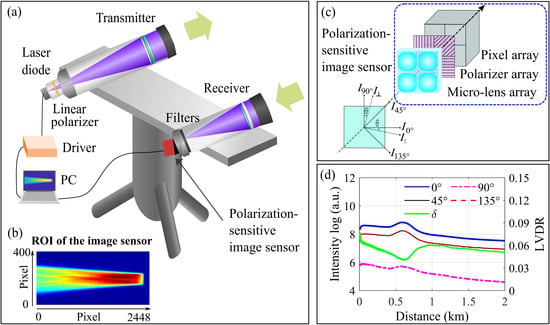
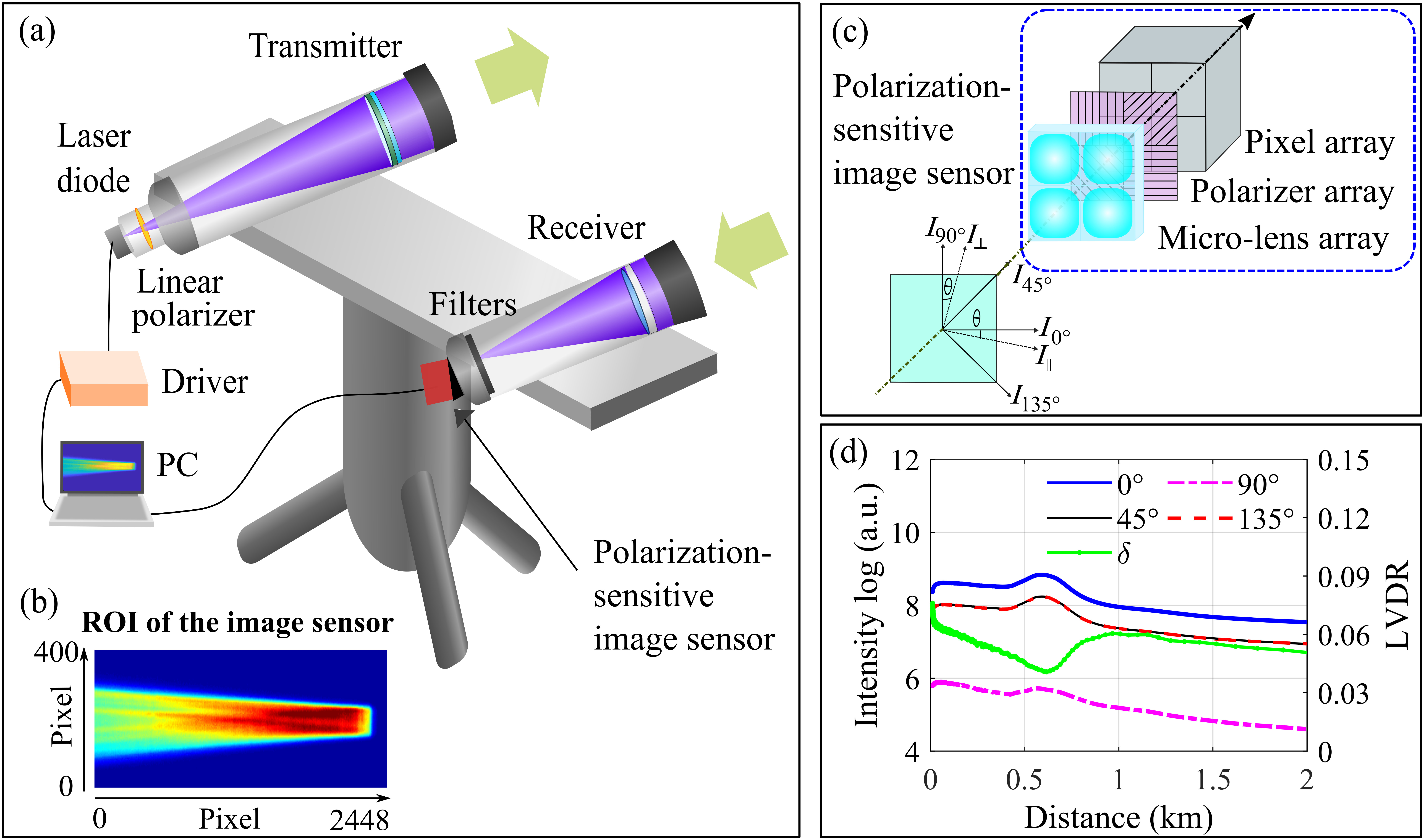
2.1. The Experimental Setup of the PSI-Lidar

The principle as well as the system schematic of the PSI-Lidar is shown in Figure 1a. A high-power multimode laser diode is utilized as the laser source. The linearly polarized laser beam emitted from the laser diode first passes through a linear polarizer with the polarization axis parallel to the polarization plane of the laser beam to improve the DoLP of the laser beam. The laser beam with a high-DoLP is then collimated by a refractor telescope using an achromatic lens and then transmitted into the atmosphere. The backscattering signals are collected by a receiving telescope (e.g., Newtonian telescope, refractor telescope) and then detected by a polarization-sensitive image sensor (Sony, IMX250MZR, 2448 × 2048, 3.45 μm). The polarization plane of the 0°-directional polarizer of the image sensor is often aligned with the polarization plane of the transmitted laser beam. The polarization image sensor, fabricated with four-directional on-chip polarizers at 0°, 45°, 90°, and 135°, as shown in Figure 1c, can capture a four-directional polarized image of the transmitted laser beam in one shot in Figure 1b. Four individual images with different polarization angles can be decoupled from the measured four-directional polarized image. Thus, lidar signals with four different polarization angles of 0°, 45°, 90°, and 135° can be simultaneously obtained from the corresponding polarization image after pixel binning and pixel-distance transform, from which the LVDR can be evaluated. In order to suppress the background signal, a band-pass interference filter can be installed in the optical path of the receiver. The intensity-modulation of the laser diode is synchronized with the exposure of the image sensor. The background image with the laser diode turned off can also be recorded, allowing real-time subtraction of the background signal. The pixel-range relationship is calibrated according to geometrical optics by measuring the backscattering signal from a tall building with a known distance from the lidar system [63]. Owing to the wide wavelength availability of the high-power multimode laser diodes and broadband responsivity of the polarization-sensitive image sensor, the PSI-Lidar technique can be implemented at various wavelengths from the visible to the near-infrared region, e.g., 450, 520, and 808 nm.

In previous work, a 450-nm PSI-Lidar prototype has been developed for atmospheric depolarization studies and a promising result has been achieved [62]. We hereby briefly introduce the PSI-Lidar system as an example. The 450-nm laser diode utilized has an output power of about 3.5 W. The laser beam is collimated by an achromatic lens (f = 600 mm, Φ = 100 mm), and the backscattering signal is collected by an achromatic lens (f = 100 mm, Φ = 50 mm). The polarization- sensitive image sensor is tilted for 7° with respect to the optical axis of the receiving lens. The receiver and the transmitter are mounted with an approximately 806 mm separation to each other to satisfy the Scheimpflug principle [56,57,64]. Figure 1d shows the lidar signals at different polarization angles measured by the 450-nm PSI-Lidar system as well as the corresponding LVDR profiles.

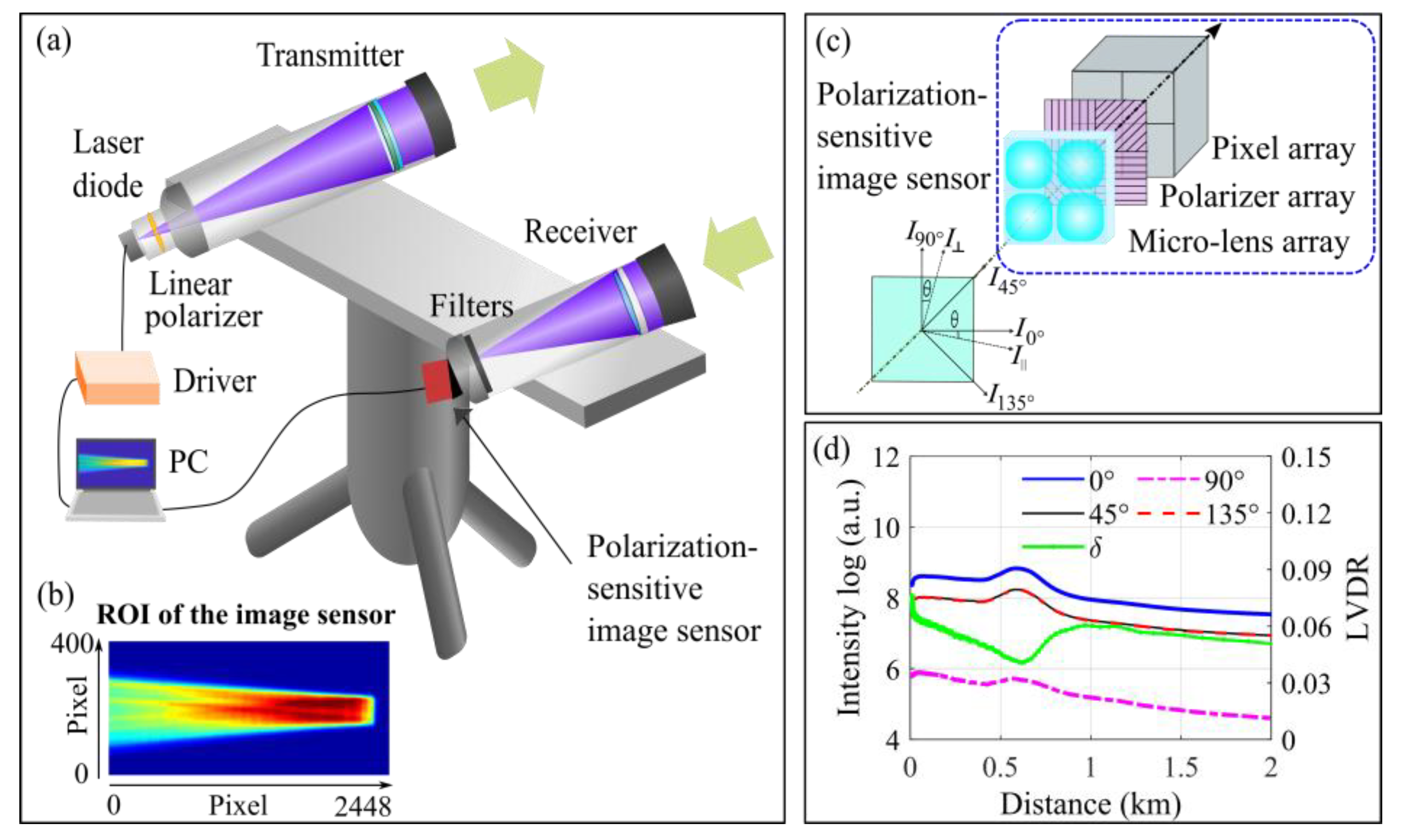
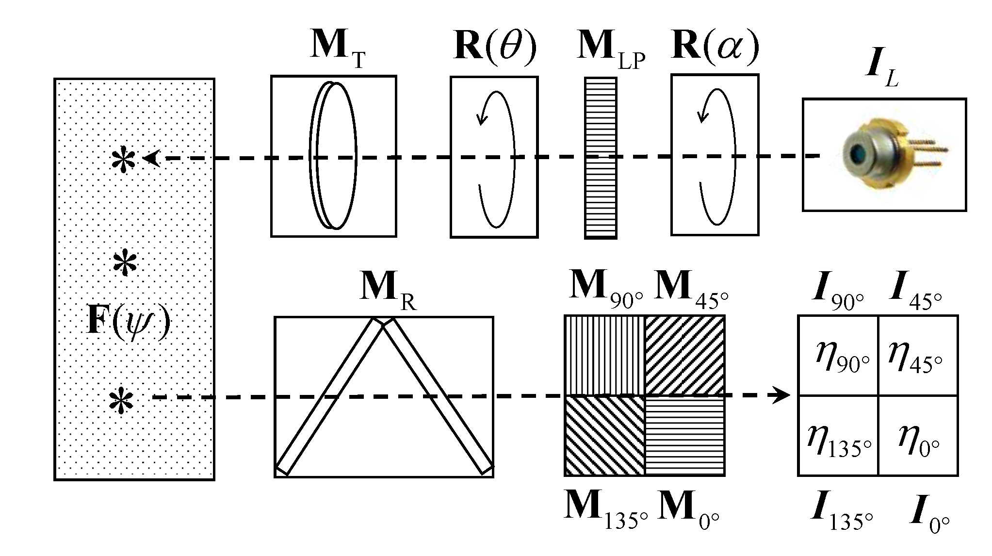
2.2. Theoretical Modeling of the PSI-Lidar

The PSI-Lidar system, from the emitted laser beam to the image sensor, can be interpreted as multiple functional modules with the corresponding Stokes vectors and Mueller matrices, as depicted in Figure 2. The Mueller matrices describe how the optical elements and the atmospheric constituents change the Stokes vectors of the laser beam. A polarization element can be described by a Mueller matrix with a combination of diattenuation, retardance, and the depolarization in general [65]. According to the principle of the polarization lidar technique and the Stokes–Mueller formalism, the Mueller matrix of the PSI-Lidar can be described as

$${\mathit{I}}_x={\eta }_x{\mathbf{M}}_x{\mathbf{M}}_{\mathbf{R}}\mathbf{F}(\psi ){\mathbf{M}}_{\mathrm{T}}\mathbf{R}(\theta ){\mathbf{M}}_{\mathrm{LP}}\mathbf{R}(\alpha ){\mathit{I}}_L$$

(1)

Here ${\mathit{I}}_{\mathrm{L}}$ is the Stokes vector describing the polarization state of the emitted laser beam from the multimode laser diode, $R(\alpha )$ and $R(\theta )$ are the rotation Mueller matrices, $\alpha$ is the rotation angle of the polarization plane of the linear polarizer with respect to the polarization plane of the laser beam, $\theta$ is the rotation angle between the polarization plane of the laser beam after passing through the linear polarizer and the 0°-directional on-chip polarizer of the polarization-sensitive image sensor, $M_{\mathrm{LP}}$ is the Mueller matrix of the linear polarizer, $M_{\mathrm{T}}$ is the Mueller matrix of the transmitter (e.g., the refractor telescope), $F(\psi )$ is the atmospheric scattering matrix with a scattering angle of $\psi$, $M_{\mathrm{R}}$ is the Mueller matrix of the receiver including the receiving telescope and the interference filters, the Mueller matrix of the polarization-sensitive image sensor can be expressed as the product between the Mueller matrix of the linear polarizer ($M_x$) and the QE of the pixel below the on-chip polarizer (${\eta }_x$), where the subscript x refers to 0°, 45°, 90°, and 135° polarization angles. In the following sections, each functional block will be described by means of Stokes-Mueller formalism.

The emitted light of the laser diode is often linearly polarized with a non-ideal PER varying in a wide range. In order to be consistent with the defined PER of the linear polarizer [65], the PER of the laser beam is defined by the ratio between the light intensity at the supposed polarization state (referred to as the parallel polarization) and the light intensity with an orthogonal polarization state (perpendicular polarization), namely

$$E{R}_L=\raisebox{1ex}{$I_0^{\parallel }$}\!\left/ \!\raisebox{-1ex}{$I_0^{\perp }$}\right.$$

(2)

Here, $I_0^{\parallel }$ and $I_0^{\perp }$ are the parallel and perpendicular polarized light intensities. The total radiation intensity ($I_0$) of the laser diode can be regarded as the sum of the parallel and perpendicular polarized lights

$$I_0=I_0^{\parallel }+I_0^{\perp }$$

(3)

The Stokes vector, describing the flux and the polarization state of a laser beam, can be generally written as $S={\left[S_0,S_1,S_2,S_3\right]}^{\mathrm{T}}$. The four elements in the vector describe the total intensity ($S_0$), the intensity difference on the x (parallel) and y (perpendicular) axes ($S_1$), the intensity difference on the +45° and −45° axes ($S_2$), and the intensity that is right-hand circular (RHC) or left-hand circular (LHC) ($S_3$), respectively [51,65]. Another parameter describing the polarization property of a laser beam is the DoLP, which is mathematically given by [66]

$$p_{\mathrm{Laser}}=\frac{\sqrt{S_1^2+S_2^2}}{S_0}=\frac{I_0^{\parallel }-I_0^{\perp }}{I_0^{\parallel }+I_0^{\perp }}=\frac{E{R}_L-1}{E{R}_L+1}$$

(4)

For the laser beam emitted by a laser diode, the Stokes vector can be written by

$${\mathit{I}}_L=I_0\left(\begin{array}{c}1\\ p_{\mathrm{Laser}}\\ 0\\ 0\end{array}\right)$$

(5)

In the PSI-Lidar technique, a linear polarizer with a high-PER may be used to improve the DoLP of the transmitted laser beam. However, most likely the polarization plane of the laser beam is not perfectly aligned with the polarization axis of the linear polarizer. If the angle between the polarization axis of the linear polarizer and the polarization plane of the emitted laser beam from the multimode laser diode is denoted as $\alpha$, the rotation Mueller matrix of the linear polarizer can be written as [54]

$$\mathit{R}(\alpha )=\left(\begin{array}{cccc}1& 0& 0& 0\\ 0& \cos 2\alpha & -\sin 2\alpha & 0\\ 0& \sin 2\alpha & \cos 2\alpha & 0\\ 0& 0& 0& 1\end{array}\right)$$

(6)

A non-idealized linear polarizer in practice has diattenuation and retardance, which can be described by the combination of the diattenuator and retarder through the Mueller matrix [65]

$$M_{\mathrm{LP}}{=\mathrm{T}}_{\mathrm{LP}}\left(\begin{array}{cccc}1& D_{\mathrm{LP}}& 0& 0\\ D_{\mathrm{LP}}& 1& 0& 0\\ 0& 0& \sqrt{1-{D_{\mathrm{LP}}}^2}\cos {\mathsf{\Delta }}_{\mathrm{LP}}& \sqrt{1-{D_{\mathrm{LP}}}^2}\sin {\mathsf{\Delta }}_{\mathrm{LP}}\\ 0& 0& -\sqrt{1-{D_{\mathrm{LP}}}^2}\sin {\mathsf{\Delta }}_{\mathrm{LP}}& \sqrt{1-{D_{\mathrm{LP}}}^2}\cos {\mathsf{\Delta }}_{\mathrm{LP}}\end{array}\right)$$

(7)

$${\mathrm{T}}_{\mathrm{LP}}=\frac{{\mathrm{T}}_{\mathrm{LP}}^{\max }+{\mathrm{T}}_{\mathrm{LP}}^{\min }}{2}=\frac{{\mathrm{T}}_{\mathrm{LP}}^{\max }\left(1+1/E{R}_{\mathrm{LP}}\right)}{2}$$

(8)

$$D_{\mathrm{LP}}=\frac{{\mathrm{T}}_{\mathrm{LP}}^{\max }-{\mathrm{T}}_{\mathrm{LP}}^{\min }}{{\mathrm{T}}_{\mathrm{LP}}^{\max }+{\mathrm{T}}_{\mathrm{LP}}^{\min }}=\frac{E{R}_{\mathrm{LP}}-1}{E{R}_{\mathrm{LP}}+1}$$

(9)

Here, ${\mathrm{T}}_{\mathrm{LP}}$ is the intensity transmittance, ${\mathrm{T}}_{\mathrm{LP}}^{\max }$ and ${\mathrm{T}}_{\mathrm{LP}}^{\min }$ are the maximum and minimum intensity transmittances of the linear polarizer with respect to the incident plane, $D_{\mathrm{LP}}$ is the diattenuation, ${\mathsf{\Delta }}_{\mathrm{LP}}$ is the phase retardance.

The polarization plane of the laser beam passing through the linear polarizer may have an offset angle of $\theta$ with respect to the 0°-directional on-chip polarizer of the polarization image sensor, which can be described by a rotation Mueller matrix

$$R(\theta )=\left(\begin{array}{cccc}1& 0& 0& 0\\ 0& \cos 2\theta & -\sin 2\theta & 0\\ 0& \sin 2\theta & \cos 2\theta & 0\\ 0& 0& 0& 1\end{array}\right)$$

(10)

In the PSI-Lidar technique, the laser beam emitted from the high-power laser diode is often collimated by an achromatic lens (or refractor telescope with achromatic lens) in order to reduce the divergence of the transmitted laser beam. The Mueller matrix of achromatic lenses is given by

$$M_{\mathrm{T}}{=\mathrm{T}}_{\mathrm{T}}\left(\begin{array}{cccc}1& D_{\mathrm{T}}& 0& 0\\ D_{\mathrm{T}}& 1& 0& 0\\ 0& 0& \sqrt{1-{D_{\mathrm{T}}}^2}\cos {\mathsf{\Delta }}_{\mathrm{T}}& \sqrt{1-{D_{\mathrm{T}}}^2}\sin {\mathsf{\Delta }}_{\mathrm{T}}\\ 0& 0& -\sqrt{1-{D_{\mathrm{T}}}^2}\sin {\mathsf{\Delta }}_{\mathrm{T}}& \sqrt{1-{D_{\mathrm{T}}}^2}\cos {\mathsf{\Delta }}_{\mathrm{T}}\end{array}\right)$$

(11)

Here, ${\mathrm{T}}_{\mathrm{T}}$ is the intensity transmittance of the achromatic lens, $D_{\mathrm{T}}$ and ${\mathsf{\Delta }}_{\mathrm{T}}$ are the diattenuation and the phase retardance of the achromatic lens, respectively.

The atmospheric scattering volume can be described by the size, shape, composition, orientation, and symmetry of the particles [67]. In this work, the atmospheric scattering volume is assumed as randomly oriented, axially symmetric scatterers [68], and the scattering angle ($\psi$) is approximately equal to 180° for typical PSI-Lidar systems that can be considered as constant. The corresponding scattering matrix can be written by [69]

$$\mathrm{F}(\pi {)=\mathrm{F}}_{11}\left(\begin{array}{cccc}1& 0& 0& 0\\ 0& 1-d& 0& 0\\ 0& 0& d-1& 0\\ 0& 0& 0& 2d-1\end{array}\right)$$

(12)

$$d=\frac{2\delta }{1+\delta }$$

(13)

Here, F₁₁ is the volume backscatter coefficient ($\beta$) and d is the depolarization parameter related to the propensity of the scattering medium to preserve the incident polarization with a range of 0–1 [69]. $\delta$ is the atmospheric LVDR, which is the primary parameter obtained from the PSI-Lidar.

Since the receiver module consists of the receiving telescope and narrowband interference filter, the Mueller matrix of the receiver module is the matrix product of the two matrices as

$$M_R=M_{\mathrm{Tel}.}{M}_{\mathrm{Filter}}{=\mathrm{T}}_R\left(\begin{array}{cccc}1& D_R& 0& 0\\ D_R& 1& 0& 0\\ 0& 0& Z_R\cos {\mathsf{\Delta }}_R& Z_R\sin {\mathsf{\Delta }}_R\\ 0& 0& -Z_R\sin {\mathsf{\Delta }}_R& Z_R\cos {\mathsf{\Delta }}_R\end{array}\right)$$

(14)

Here, ${\mathrm{T}}_R$, $D_R$, $Z_R$ and ${\mathsf{\Delta }}_R$ are given by

$${\mathrm{T}}_R={\mathrm{T}}_{\mathrm{Tel}.}{\mathrm{T}}_{\mathrm{Filter}}(1+D_{\mathrm{Tel}.}{D}_{\mathrm{Filter}})$$

(15)

$$D_R=\frac{D_{\mathrm{Tel}.}+D_{\mathrm{Filter}}}{1+D_{\mathrm{Tel}.}{D}_{\mathrm{Filter}}}$$

(16)

$$Z_R=\frac{\sqrt{1-D_{\mathrm{Tel}.}^2}\sqrt{1-D_{\mathrm{Filter}}^2}}{1+D_{\mathrm{Tel}.}{D}_{\mathrm{Filter}}}$$

(17)

$${\mathsf{\Delta }}_R={\mathsf{\Delta }}_{\mathrm{Tel}.}+{\mathsf{\Delta }}_{\mathrm{Filter}}$$

(18)

Here, ${\mathrm{T}}_{\mathrm{Tel}.}$ and ${\mathrm{T}}_{\mathrm{Filter}}$ are the intensity transmittances of the receiving telescope and narrowband interference filter, respectively. $D_R$ and ${\mathsf{\Delta }}_R$ are the diattenuation and the phase retardance of the receiving module, respectively.

The polarization-sensitive image sensor consists of pixel (photo-detector) arrays and on-chip linear polarizers that are fabricated between the micro-lens and the photodetector. The linear polarizer for a specific polarization angle can be described by the Mueller matrix

$${{\rm M}}_x{=\mathrm{T}}_x\left(\begin{array}{cccc}1& D_x& 0& 0\\ D_x& 1& 0& 0\\ 0& 0& \sqrt{1-{D_x}^2}\cos {\mathsf{\Delta }}_x& \sqrt{1-{D_x}^2}\sin {\mathsf{\Delta }}_x\\ 0& 0& -\sqrt{1-{D_x}^2}\sin {\mathsf{\Delta }}_x& \sqrt{1-{D_x}^2}\cos {\mathsf{\Delta }}_x\end{array}\right)$$

(19)

Here, the subscript x refers to 0°, 45°, 90°, and 135° polarization angle, ${\mathrm{T}}_x$ is the intensity transmittances of the linear polarizer, respectively, $D_x$ and ${\mathsf{\Delta }}_x$ are the diattenuation and the phase retardance of the linear polarizer, respectively.

According to the above equations, the relationship between the detected lidar signals (${\mathit{I}}_x$) at four different polarization angles and the LVDR can be established by the Stokes vectors and the Mueller matrices. The measurement errors introduced by the DoLP of the laser beam, the offset angle between the polarization plane of the transmitted laser beam and the 0°-directional polarizer of the image sensor, the QE and the PER of the image sensor can thus be evaluated through the Stokes–Mueller formalism.

3. Optical Parameters of the PSI-Lidar

The polarization-sensitive image sensor can capture a four-directional polarized image in one shot. Thus, lidar signals at four different polarization angles can be simultaneously obtained from the polarization-sensitive image sensor, from which the LVDR can be evaluated according to the Stokes–Mueller formulas. Nevertheless, as discussed in Section 2, the retrieval of the LVDR depends on many system factors of the PSI-Lidar system, such as the DoLP of the laser beam, the QE and the PER of the polarization-sensitive image sensor, etc. The systematic errors of the PSI-Lidar technique thus arise from the uncertainties of these system parameters, which should be determined.

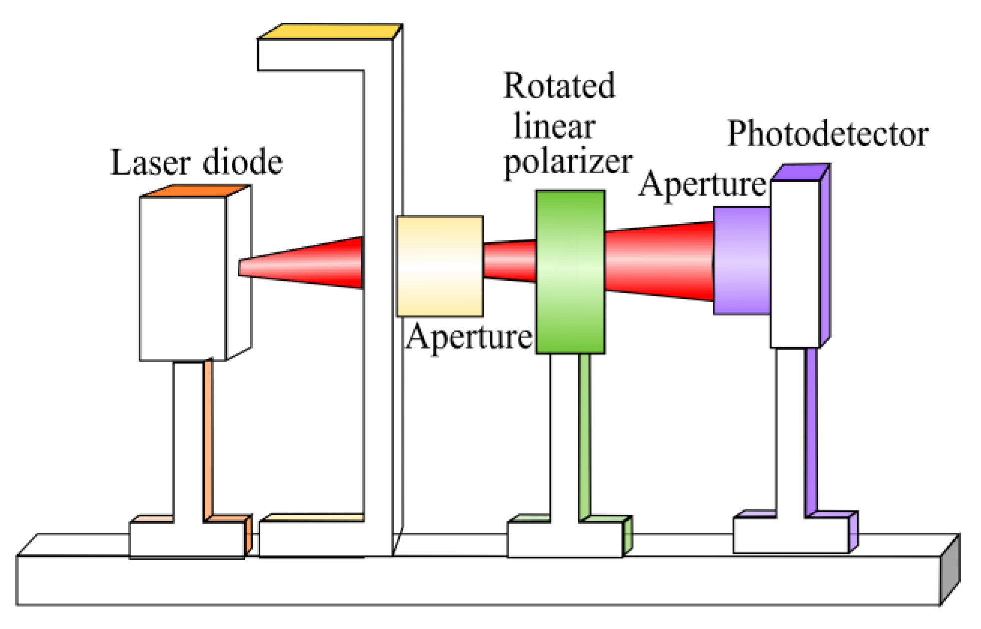
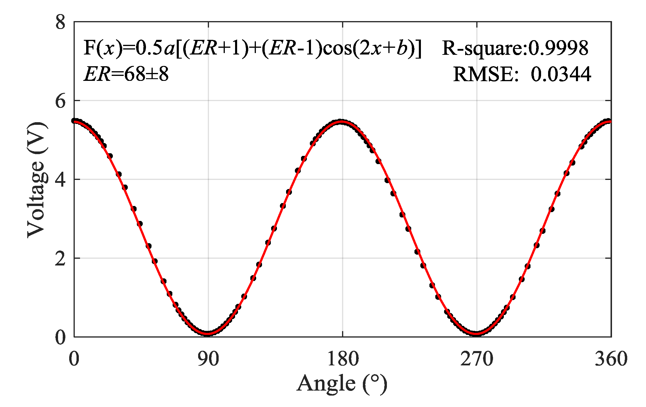
3.1. The DoLP of the Laser Beam

Table 1. The PER as well as the corresponding DoLP for multimode laser diodes at different wavelengths. The PER and DoLP of 808 nm were measured by the experimental setup shown in Figure 3.

Laser Diode	450 nm	450 nm	520 nm	808 nm
Supplier	Osram	Thorlabs	Thorlabs	Huaguang Optoelectronics
Model	PL TB450B	L450G1	L520G1	C-mount
Output power	1.6 W	3.2 W	0.9 W	5 W
PER	400:1	100:1	300:1	68 ± 8:1
DoLP	0.9950	0.9802	0.9934	>0.9672

gives the PER as well as the corresponding DoLP of multimode laser diodes at different wavelengths, which are obtained from datasheets provided by the suppliers. As can be seen, the PER of multimode laser diodes at 450 and 520 nm are typically in the region of 100-400 leading to a DoLP beyond 0.98. However, the PER value of the 808-nm laser diode is seldom provided by manufacturers. Thus, an experimental setup was developed to measure the PER (DoLP) of the laser beam emitted from the 808-nm laser diode. As shown in Figure 3, the laser beam emitted by the laser diode first passed through an 1-mm aperture and then a high-PER linear polarizer (>10,000:1), which can be considered as an ideal polarizer. A second aperture was installed in front of the amplified photodetector to suppress the stray light. The transmission intensity of the polarized laser beam through the linear polarizer was detected by the photodetector and then acquired by a data acquisition (DAQ) card for data analysis. The linear polarizer was manually rotated through a rotational polarizer mount from 0° to 360° with a step of 2°, and the transmission intensity through the linear polarizer is recorded for 8 s at each rotation angle of the linear polarizer. Figure 4 shows the relationship between the detected intensities and the rotation angles of the linear polarizer. The PER can be obtained by fitting the polarization response curve according to a cosine function. It has been found out that the PER of the 808 nm laser diode is about 68 ± 8, which is much smaller than those at shorter wavelengths.

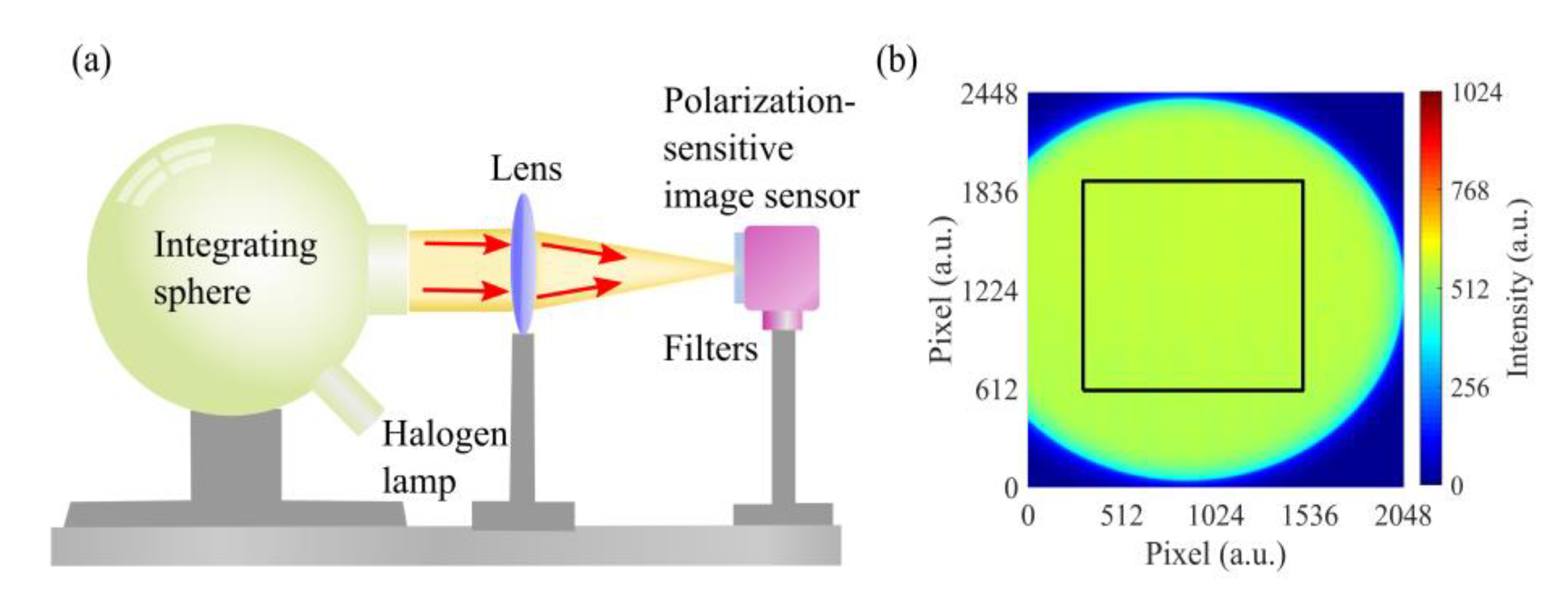
3.2. The Relative Quantum Efficiencies (QEs) of the Polarization-Sensitive Image Sensor

The relative QEs of the four polarization channels of the image sensor also has a direct impact on the measurement results, as indicated by Equation (1). Although the relative QEs of the image sensor can be obtained directly from its datasheet, it is worthwhile to further investigate the dependency of the relative QEs on the total illumination intensity of the incoming light, which can vary substantially during atmospheric measurements. The experimental setup for measuring the relative QE of the four-directional polarization channels is shown in Figure 5a. An integrating sphere with a halogen light source is utilized to create a near-ideal unpolarized light. A convex lens with a diameter of 50 mm and a focal length of 100 mm can focus the unpolarized light emitted by the integrating sphere on the polarization-sensitive image sensor. As the halogen light source has a wide emission spectrum from 400–1000 nm, different interference filters were utilized to select the emission spectrum, e.g., 450 nm interference filter (FWHM = 10 nm), 520 nm interference filter (FWHM = 10 nm), and 808 nm interference filter (FWHM = 3.1 nm) with an RG780 long-pass filter, which were placed in front of the image sensor. The cone half-angle (CHA) of the incident light to the image sensor was about ±5°.

The image of the unpolarized light was recorded with different exposure times ranging from 20 to 400 ms to investigate the influence of different illumination intensities. Meanwhile, 20 frames were acquired at each exposure time to perform image averaging and thus to improve the signal-to-noise ratio (SNR). Figure 5b shows a typical image recorded by the image sensor. The uniform part of the image, marked with a rectangle, referred to as the region of interest (ROI), was chosen to evaluate the relative QEs. The image in the ROI was decoupled into four directional polarized images. The relative QE for each individual pixel in the ROI was then evaluated from the ratio between the light intensity for a specific polarization angle and the mean light intensity of all polarization angles. The relative QEs for all pixels in the ROI may deviate slightly owing to the photon-response nonuniformity (PRNU) of the image sensor, which is also susceptive to the illumination intensity [70]. The measurement result revealed that the standard deviation of the relative QEs for the pixels in the ROI is less than 0.8% for high light-level condition (incoming light intensity is more than 10% of the full well capacity of each pixel), while it could increase to 1.3% for low light level condition. Nevertheless, the pixel-to-pixel variation of the relative QE is considered as random noise for lidar signal. Meanwhile, the image of the laser beam is vertically binned to obtain the lidar profile in practical lidar measurements, which can also greatly suppress the influence of the PRNU. Thus, the mean value of the relative QE for all pixels in the ROI is more appropriate for the evaluation of the depolarization ratio. The final relative QE is taken from the average value of the six-time measurements with different exposure times, and the standard deviation indicates the variation of the relative QE with the illumination intensity.

The measured relative QEs as well as the values from the datasheet at three different wavelengths are shown in

Table 2. The measured relative QEs as well as the relative QEs obtained from the manufacture datasheet (factory relative QEs) at 450, 520, and 808 nm. The deviations of the measured relative QEs are evaluated from six-time measurements with different exposure times varying from 20 to 400 ms.

Wavelengths	Polarized Channel	Relative QEs Calculated from Measurements	Relative QEs from Datasheet	Relative Bias
450 nm with a bandwidth of 10 nm	0°	0.9832 ± 0.0002	0.982	0.12%
	90°	0.9805 ± 0.0004	0.981	0.05%
	45°	1.0242 ± 0.0003	1.024	0.02%
	135°	1.0121 ± 0.0002	1.013	0.08%
520 nm with a bandwidth of 10 nm	0°	0.9897 ± 0.0001	0.988	0.17%
	90°	0.9844 ± 0.0003	0.985	0.06%
	45°	1.0168 ± 0.0002	1.020	0.31%
	135°	1.0091 ± 0.0002	1.006	0.31%
808 nm with a bandwidth of 3.1 nm	0°	0.9937 ± 0.0001	0.980	1.40%
	90°	0.9823 ± 0.0003	0.999	1.67%
	45°	1.0050 ± 0.0001	1.014	0.89%
	135°	1.0190 ± 0.0003	1.007	1.19%

. In general, the measured relative QEs were in good agreement with those provided by the datasheet. The deviations of the relative QEs between the measured values and the factory values at 450, 520, and 808 nm are less than 0.2%, 0.31%, and 2%, respectively. Meanwhile, the fluctuation of the measured relative QE is less than 0.04% when the total illumination intensity varied from 5% to 80% of the full-well capacity (FWC) of the image sensor. This implies that the relative QE is independent of the illumination intensity, which is of great benefit for employing the polarization-sensitive image sensor for depolarization studies.

3.3. The Polarization Extinction Ratios (PERs) of the Polarization-Sensitive Image Sensor

According to the datasheet of the polarization-sensitive image sensor, the PER varies from 40 to 470 in the region of 400–900 nm and it could also deviate at different polarization angles.

Table 3. The PERs of the image sensor at different wavelengths, obtained from the datasheet of the polarization-sensitive image sensor.

Polarization Angle	450 nm	520 nm	808 nm
0°	467	338	74
90°	469	331	74
45°	414	306	107
135°	434	301	60

shows the PERs of different polarization angles at three different wavelengths, obtained from the datasheet of the polarization-sensitive image sensor. As can be seen, the PER at 808 nm is significantly smaller than those in the blue-green region. Due to the non-ideal PER, crosstalk between different polarization states could occur. For instance, the 90° polarization channel (or pixel) may detect the parallel polarized backscattering signal, leading to the overestimation of the 90° polarization signal. The overestimation can result in a measurement error comparable to the molecular depolarization ratio (typically about 0.004). Thus, it is of great importance to investigate the polarization crosstalk effect on the polarized lidar signals.

4. Evaluation and Discussion of Systematic Errors for the PSI-Lidar

In this section, systematic errors introduced by various factors, e.g., the DoLP of the emitted laser beam, the offset angle, the QEs and the PERs of the polarization-sensitive image sensor, were analyzed and discussed. The systematic errors introduced by the transmitter, e.g., the small depolarizing effect of the achromatic lens, are neglected as the uncertainty introduced by possible birefringence is very difficult to analyze and estimate [54]. Furthermore, the polarization effects of the receiver, e.g., telescope, are neglected in this work [71,72]. Even so, the analysis framework presented below is feasible to include such effects. It should be noted that the polarization crosstalk of a Cassegrain telescope with small incidence angles of the incoming light in lidar is negligible, guiding us to choose an optimal receiving telescope to reduce the systematic error [52].

4.1. The Systematic Error Introduced by the DoLP of the Transmitted Laser Beam

The LVDR can be significantly influenced by the crosstalk between lights with different polarization states originating from the non-ideal polarization property (DoLP < 1) of the laser beam that has been transmitted into the atmosphere. According to Stokes–Mueller formalism, the DoLP-related relative error of the LVDR can be deduced by neglecting the influence from other factors

$${\epsilon }_{\mathrm{DoLP}}=\left|{\delta }_0-\frac{\left(1+{\delta }_0\right)-\left(1-{\delta }_0\right)p_{\mathrm{Trans}.}}{\left(1+{\delta }_0\right)+\left(1-{\delta }_0\right)p_{\mathrm{Trans}.}}\right|/{\delta }_0$$

(20)

Here, $p_{\mathrm{Trans}.}$ is the DoLP of the laser beam that is transmitted into the atmosphere, ${\delta }_0$ is the true value of the LVDR, which is only dependent on the optical properties of the scatters (see Equation (12)). Figure 6 illustrates the relationship between the relative error and the DoLP of the transmitted laser beam at typical atmospheric LVDRs for molecules (0.004), anthropogenic aerosol (0.05), and dust (0.3) [35,73,74]. As can be seen, the relative error decreases with the increasing of the DoLP, and increases when the LVDR becomes smaller. It can be concluded that the relative error of the LVDR would be limited to 1% even in the case of molecular depolarization ratio (≈0.004) if the DoLP of the transmitted laser beam can reach up to 99.992%.

According to the PERs of the multimode laser diode shown in Table 1, the relative error can reach up to 250% at 450 nm (3.2 W), 83% at 520 nm, and 417% at 808 nm with a molecular depolarization ratio of about 0.004. Thus, a linear polarizer has to be utilized to improve the DoLP of the transmitted laser beam as well as the systematic error. The DoLP of the laser beam after passing through a linear polarizer is given by

$$p_{\mathrm{Trans}.}=\frac{(E{R}_{\mathrm{LP}}-1)+(E{R}_{\mathrm{LP}}+1)p_{\mathrm{Laser}}\cos (2\alpha )}{(E{R}_{\mathrm{LP}}+1)+(E{R}_{\mathrm{LP}}-1)p_{\mathrm{Laser}}\cos (2\alpha )}$$

(21)

Here, $p_{\mathrm{Laser}}$ is the DoLP of the laser beam emitted from the multimode laser diode. As can be seen, the DoLP of the transmitted laser beam is primarily determined by the PER of the linear polarizer ($E{R}_{\mathrm{LP}}$), the rotation angle ($\alpha$) as well as the original DoLP of the emitted laser beam from the multimode laser diode. The rotation angle can be readily controlled to ±2° through manual alignment with a fine dial. For a laser diode with a small PER of 68 (e.g., 808-nm laser diode), the DoLP of the transmitted laser beam can reach up to 99.992% by using a linear polarizer with a PER of 500:1, which is widely available. In summary, the systematic error introduced by the non-ideal polarized laser beam of multimode laser diodes can be neglected by employing a relatively high-PER linear polarizer to improve the DoLP of the transmitted laser.

4.2. The Systematic Error Introduced by the Polarization-Sensitive Image Sensor

4.2.1. The Systematic Error Introduced by the Relative QEs of the Four Polarization Channels

The relative QEs directly influence the ratio between lidar signals measured at different polarization angles and thus the value of the LVDR. In order to investigate the potential systematic error introduced by the relative QEs, the LVDRs are evaluated with the measured relative QEs and the factory relative QEs, respectively, while the contributions from other optical components are not taken into account. The deviation of the LVDR evaluated with different relative QEs is given by

$${\epsilon }_{\mathrm{QE}}=\frac{\left|{\delta }_{\mathrm{Meas}.}-{\delta }_{\mathrm{Data}}\right|}{{\delta }_{\mathrm{Meas}.}}=\frac{\left|\left({\eta }_{0°}^{\mathrm{Meas}.}{\eta }_{90°}^{\mathrm{Data}}-{\eta }_{0°}^{\mathrm{Data}}{\eta }_{90°}^{\mathrm{Meas}.}\right){\eta }_{90°}^{\mathrm{Meas}.}\right|}{{\eta }_{90°}^{\mathrm{Meas}.}{\eta }_{90°}^{\mathrm{Data}}{\eta }_{0°}^{\mathrm{Meas}.}}$$

(22)

Here, ${\delta }_{\mathrm{Meas}.}$ is the LVDR evaluated with the measured relative QEs (${\eta }_{0°}^{\mathrm{Meas}.}$, ${\eta }_{90°}^{\mathrm{Meas}.}$), and ${\delta }_{\mathrm{Data}}$ is the LVDR calculated with the factory relative QEs (${\eta }_{0°}^{\mathrm{Data}}$, ${\eta }_{90°}^{\mathrm{Data}}$). The deviation of the LVDR is generally less than 0.3% at 450 and 520 nm, but slightly larger at 808 nm, i.e., about 3%. Nevertheless, these small deviations can be neglected for practical measurements of LVDR. Moreover, the influence of different illumination intensities is also negligible, since the relative QEs is independent of the illumination intensity, as was discussed in Section 3.2. The small deviations also imply that the influence of the relative QEs on the LVDR can be well-calibrated from either experimental or factory relative QEs.

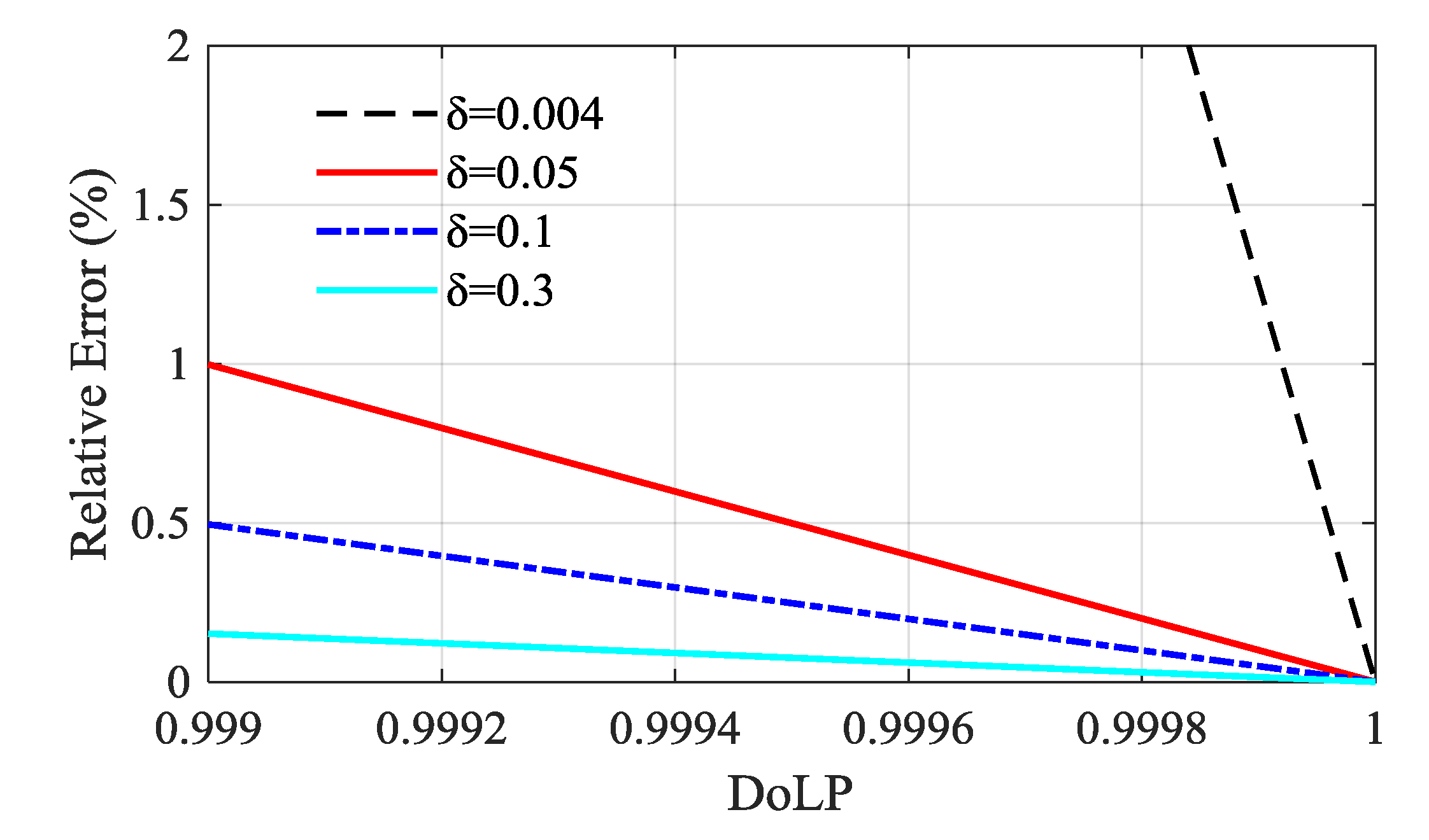
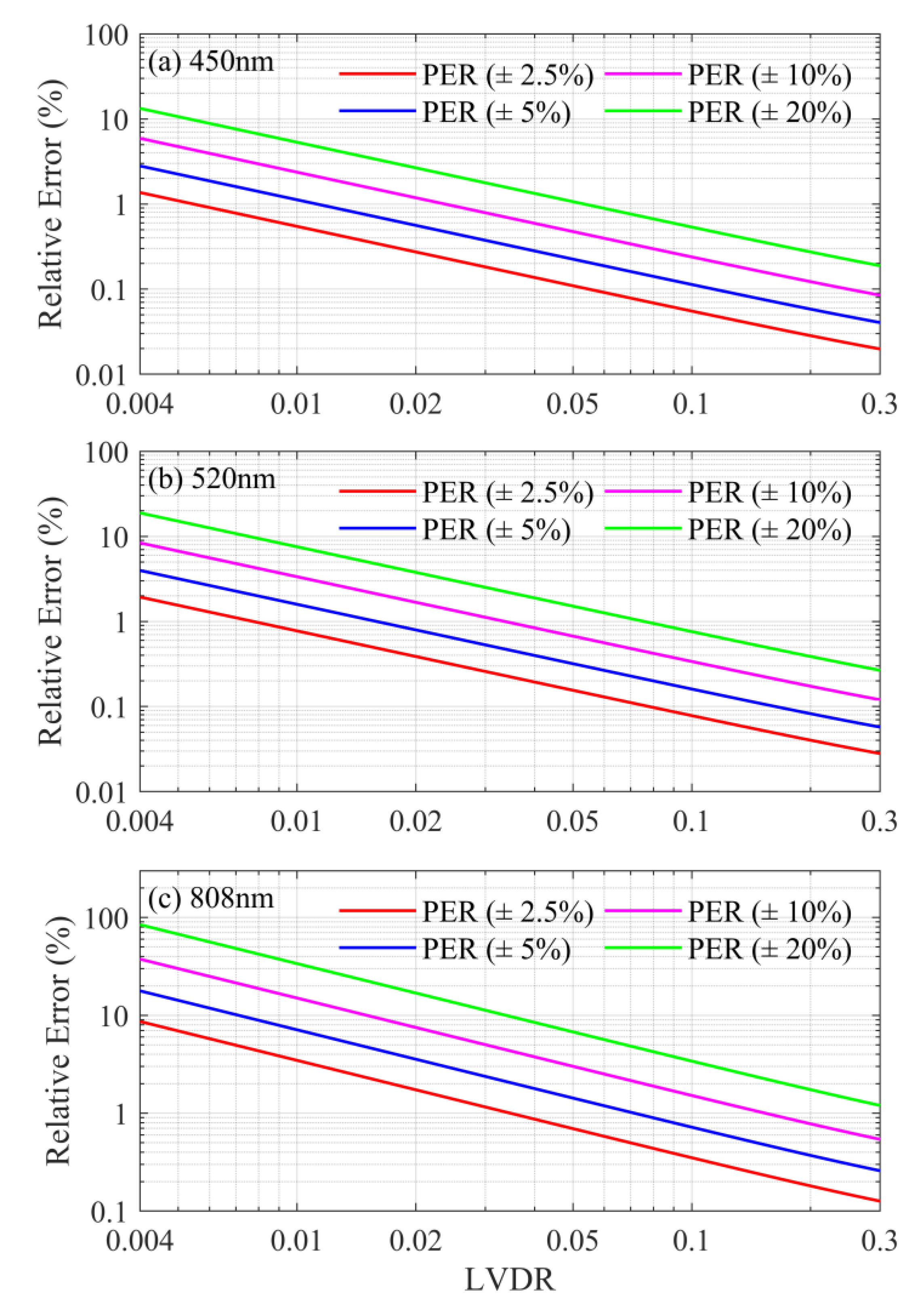
4.2.2. The Systematic Error Introduced by the Non-Ideal PERs of the Image Sensor

Owing to the non-ideal PERs of the image sensor, there would be crosstalk for the lidar signals detected at different polarization angles, leading to considerable systematic errors. However, there are some differences between the crosstalk effect of the conventional polarization pulsed lidar technique based on the PBS and the PSI-Lidar technique, which are worthwhile to elaborate. In conventional polarization lidar technique, the backscattering beam is divided into parallel and perpendicular polarized beams through a PBS. Owing to the non-ideal PER of the PBS, crosstalk can occur, e.g., the parallel polarized laser beam may contain the light with perpendicular polarization state and vice versa. Nevertheless, the sum intensity of the two orthogonally polarized laser beams is equal to the intensity of the backscattering beam before entering the PBS. On the other hand, in the PSI-Lidar technique, the backscattering laser beam is detected simultaneously by many polarized pixels that are spatially spaced as shown in Figure 1c. The incident light on a specific pixel will have a maximum transmission if its polarization state is parallel to the polarization angle of the corresponding on-chip linear polarizer, and a minimum transmission for the light with perpendicular polarization. The primary part of the perpendicular polarized light is rejected by the on-chip linear polarizer, which will not be detected by the photodiode fabricated below the linear polarizer. The crosstalk effect is mainly determined by the PER value of the on-chip linear polarizer. Assuming that other optical components are ideal and the atmospheric particles are randomly oriented, axially symmetric scatterers, the relative error (${\epsilon }_{\mathrm{ER}}$) of the LVDR introduced by ignoring the crosstalk effect can be expressed by

$${\epsilon }_{\mathrm{ER}}=\left|{\delta }_0-\frac{{\delta }_0+1/E{R}_{90°}}{1+{\delta }_0/E{R}_{0°}}\right|/{\delta }_0$$

(23)

Here, ${\delta }_0$ is the true value of the LVDR, $E{R}_{0°}$ and $E{R}_{90°}$ are the extinction ratios of the 0°- and 90°-linear polarizers, described by ${\mathrm{T}}_{0°}^{\max }/{\mathrm{T}}_{0°}^{\min }$ and ${\mathrm{T}}_{90°}^{\max }/{\mathrm{T}}_{90°}^{\min }$, respectively. In the following discussions, $E{R}_{0°}$ and $E{R}_{90°}$ are also referred to as 0°-PER and 90°-PER, respectively.

Table 4. The relative errors introduced by ignoring the crosstalk effect owing to the non-ideal PERs of the on-chip linear polarizer at different LVDRs.

LVDR	PER: 467 at 0° 469 at 90° at 450 nm	PER: 338 at 0° 331 at 90° at 520 nm	PER: 74 at 0° 74 at 90° at 808 nm
0.004	53%	76%	338%
0.05	4%	6%	27%
0.1	2%	3%	13%
0.3	0.7%	0.9%	4%

shows the relative error of the LVDR introduced by ignoring the crosstalk effect due to non-ideal PERs. If the value of the LVDR is beyond 0.05, the relative error introduced by ignoring the crosstalk effect is less than 6% in the blue-green region and less than 27% in the near-infrared region. Meanwhile, the relative error at 808 nm considerably decreases with the increasing of the LVDR, and it is about 4% for a LVDR of 0.3. In clean atmospheric conditions dominated by molecules, the value of the LVDR could be smaller than 0.01, e.g., 0.004. In this case, the relative errors for all wavelengths increase significantly, up to about 338% at 808 nm, 76% at 520 nm, and 53% at 450 nm, as the crosstalk effect is comparable to the atmospheric depolarization effect, which should be carefully considered. In fact, the relative error of the LVDR is the tradeoff result between the crosstalk effect and the atmospheric depolarization effect.

If the crosstalk effect is taken into account, the measured LVDR can be mathematically given by

$${\delta }_{\mathrm{Meas}.}=\frac{\left(I_{90°}/I_{0°}\right)-1/E{R}_{90°}}{1-\left(I_{90°}/I_{0°}\right)/E{R}_{0°}}$$

(24)

In principle, as long as the PER of the image sensor can be precisely obtained, the influence of the crosstalk effect on the measured LVDR can be readily eliminated according to Equation (24). In other words, ${\delta }_{\mathrm{Meas}.}$ is equal to the true value of the LVDR, namely ${\delta }_{\mathrm{Meas}.}={\delta }_0$. Although the PER values can be obtained from the datasheet provided by the manufacturer, the polarization characteristic may not be guaranteed the same for every product due to differences in production batches. The uncertainty or deviation of the PER with respect to the factory or true value can thus introduce a certain amount of error on the retrieved LVDR. The relative error of the LVDR due to the uncertainty of the PERs of the image sensor can thus be expressed by

$${\epsilon }_{\mathrm{ER}}=\left|{\delta }_{\mathrm{Meas}.}(ER)-{\delta }_0\right|/{\delta }_0$$

(25)

Here, ${\delta }_{\mathrm{Meas}.}(ER)$ is the LVDR evaluated with an arbitrary PER in the uncertainty region of the true PER.

Simulation studies were carried out to investigate the influence of the PER uncertainty on the basis of the factory or true PER value. The relative errors of the LVDR due to the uncertainties of the PERs were calculated with a LVDR value varying from 0.004 to 0.3, as shown in Figure 7. For urban aerosols or dust, the value of LVDR is often larger than 0.05 and can reach up to 0.3 [35,74]. Under these circumstances, the relative error can be limited to 1.5% at 450 and 520 nm even if the uncertainty of the PER reaches up ±20%, while the relative error is less than 7% at 808 nm. In order to achieve the above relative error level (e.g., 1.5%) at around 808 nm, the PER uncertainty at 808 nm should be limited to ±5%. If the atmosphere is dominated by molecules, the value of the LVDR is often less than 0.01 (e.g., 0.004) depending on ambient temperature, spectral width, wavelength, etc. [73]. For such a small LVDR, the relative errors at 450 and 520 nm would be less than 4% for a PER uncertainty less than ±5%. However, the relative error at 808 nm varies from 7% to 18% under the same conditions. To achieve a relative error of less than 10% for an LVDR of 0.004, the uncertainty of the PER at 808 nm should not be larger than ±2.5%. Clearly, the relative errors can be substantially reduced by taking the polarization crosstalk effect into account, particularly for the cases with small LVDRs. It can be concluded that precise information regarding the PER value of the polarization-sensitive image sensor is critical for accurate measurements of small LVDRs, particularly at 808 nm.

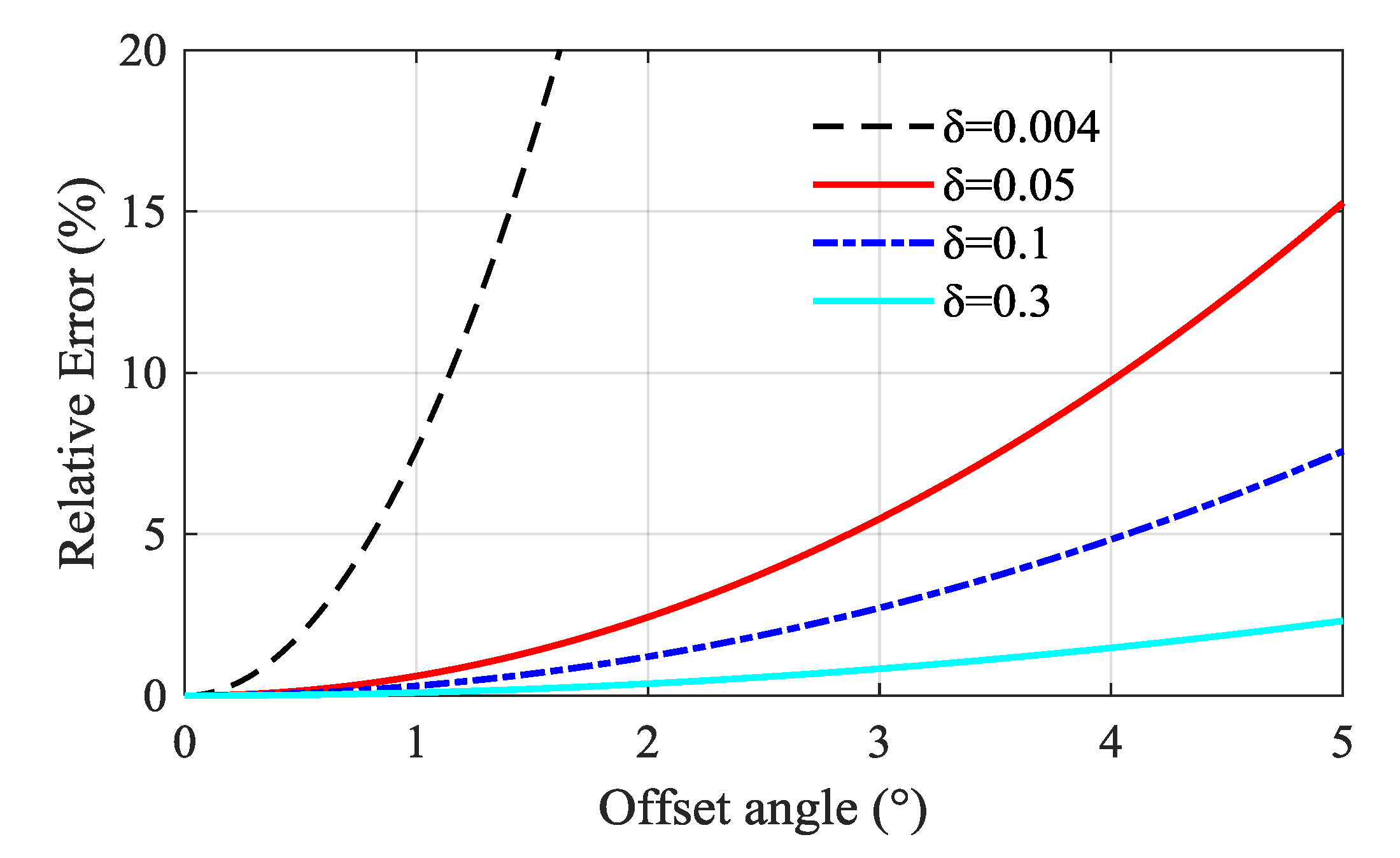
4.3. The Systematic Error Introduced by the Offset Angle

In an ideal PSI-Lidar system, the polarization plane of the transmitted laser beam would be aligned perfectly with the 0°-directional on-chip polarizer of the polarization-sensitive image sensor. However, perfect alignment is very difficult to achieve. There could be a misalignment (offset) angle ($\theta$) between the polarization plane of the transmitted laser beam and the polarization plane of the 0°-directional on-chip polarizer of the polarization-sensitive image sensor. The misalignment can cause the leakage of the parallel-polarized signal to the cross-polarized signal, leading to overestimation of the LVDR.

Assuming that the atmospheric particles are randomly oriented axially symmetric scatterers and neglecting the influence of other optical components, the relative error of the LVDR introduced by the offset angle can be deduced as

$${\epsilon }_{\mathrm{offset}}=\left|{\delta }_0-\frac{\left(1+{\delta }_0\right)-\left(1-{\delta }_0\right)\cos (2\theta )}{\left(1+{\delta }_0\right)+\left(1-{\delta }_0\right)\cos (2\theta )}\right|/{\delta }_0$$

(26)

Simulation results of the relative errors introduced by the offset angle with different offset angles and LVDRs are shown in Figure 8. As can be seen, the relative error will increase with the increasing of the offset angle. Meanwhile, the relative error may increase considerably for a small value of the LVDR. The relative error introduced by the offset angle would be limited to 5% for the molecular depolarization of around 0.004, as long as the offset angle is smaller than 0.81°. The relative error can be further reduced to below 1%, if the offset angle is in the range of ±0.37°.

In the PSI-Lidar technique, the offset angle can be determined from the polarized lidar signals at 0°-, 90°-, 45°-, and 135°-polarization angles, which is given by

$$\tan 2\theta =\frac{V_{2}E{R}_{135°}\left(E{R}_{45°}+1\right)-E{R}_{45°}\left(E{R}_{135°}+1\right)}{V_{2}E{R}_{135°}\left(E{R}_{45°}-1\right)+E{R}_{45°}\left(E{R}_{135°}-1\right)}\times \frac{E{R}_{0°}\left(E{R}_{90°}-1\right)+V_{1}E{R}_{90°}\left(E{R}_{0°}-1\right)}{E{R}_{0°}\left(E{R}_{90°}+1\right)-V_{1}E{R}_{90°}\left(E{R}_{0°}+1\right)}$$

(27)

Here, $E{R}_{45°}$ and $E{R}_{135°}$ are referred to as 45°-PER and 135°-PER, respectively. $V_1$ and $V_2$ are defined as

$$V_1=\frac{I_{90°}{\eta }_{0°}}{I_{0°}{\eta }_{90°}}$$

(28)

$$V_2=\frac{I_{135°}{\eta }_{45°}}{I_{45°}{\eta }_{135°}}$$

(29)

According to Equations (27)–(29), the offset angle can be calculated based on the four polarized lidar signals and the PER values at the four polarization angles. The retrieval error of the offset angle is primarily determined by the uncertainties of the PER values. Numerical simulation on the retrieval error of the offset angle was carried out with the PER values at each polarization angle varying ±20% in respect to the factory or true PER values. In general, the retrieval error of the offset angle increases with the increasing of the PER uncertainty.

Table 5. The retrieval error of the offset angle at different wavelengths with the LVDR varying from 0.004 to 0.3. The uncertainty of the PER is set to ±20%.

	LVDR = 0.004	LVDR = 0.05	LVDR = 0.1	LVDR = 0.3
450 nm	0.01°	0.02°	0.02°	0.03°
520 nm	0.02°	0.02°	0.02°	0.04°
808 nm	0.08°	0.09°	0.10°	0.15°

shows the retrieval error of the offset angle with a PER uncertainty of ±20% for different wavelengths and different atmospheric LVDRs. As can be seen, the retrieval error of the offset angle increases with the increasing of the atmospheric LVDR. The retrieval error at 808 nm is much larger than those at the blue-green region, due to the relatively small values of the PER. However, the maximum retrieval error of the offset angle is less than 0.15° for a LVDR value of 0.3. It can be concluded that the retrieval error of the offset angle is not very sensitive to the uncertainty of the PERs at the four polarization angles. According to the simulation results shown in Figure 8, the systematic error of LVDR with an offset-angle measurement error of 0.15° is less than 1% for a LVDR in the region of 0.0040–0.3, which can be neglected during practical polarization studies.

Since the PERs at the four-directional polarized channels are much larger than 1, Equation (27) can also be approximated by

$$\tan 2\theta \approx \frac{1+V_1}{1-V_1}\times \frac{V_2-1}{V_2+1}$$

(30)

As can be seen, the offset angle is mainly determined by the values of $V_1$ and $V_2$. Although the value of the offset angle can always be retrieved from the four polarization lidar signals, it is more preferable to have a 0° offset angle in practical depolarization measurements. A simple and efficient approach to achieve a 0° offset angle is to let the value of $V_2$ equal to 1. In other words, the offset angle equals 0°, if signal intensities at 45° and 135° polarization angles are identical after normalization by the relative QE.

5. Conclusions

In this work, a theoretical model based on the Stokes–Mueller formalism was established for the newly developed polarization-sensitive imaging lidar (PSI-Lidar) technique. The systematic errors introduced by the DoLP of the emitted laser beam, the offset angle, the relative QEs, and the PERs of the polarization-sensitive image sensor, were evaluated in detail for the PSI-Lidar at several wavelengths from the visible to the near-infrared region. The following conclusions can be summarized according to experimental as well as simulation studies.

The PERs of multimode laser diodes are often not very high, e.g., varying from about 60 to 400 (DoLP > 0.967) depending on the wavelengths, etc. Directly transmitting the laser beam emitted from the laser diode into the atmosphere can introduce a large measurement error due to the crosstalk in the image sensor for light with different polarization states, particularly for the cases with very small LVDR values. However, the influence of a non-ideal polarized laser beam on the LVDR can be reduced to less than 1% by employing a linear polarizer (PER > 500) before transmitting the laser beam into the atmosphere.

The relative QEs of the image sensor have a direct impact on the measured LVDR. Laboratory measurements have found that the relative QEs are independent of the total illumination intensity and indicates a good consistency with the factory relative QEs (less than 2% deviation). The promising result demonstrated that the influence of the relative QEs on the LVDR can be well-calibrated from either experimental or factory relative QEs. Moreover, as the four polarization channels are on-chip fabricated having good uniformity, the relative QEs of the image sensor are insensitive to ambient environment or measurement conditions, which implies that there is no need for frequent or periodical calibrations.

Owing to the non-ideal PER of the image sensor (about 74 at 808 nm, about 470 at 450 nm), the crosstalk between lights with different polarization states can significantly influence the measured LVDR, e.g., the relative error can reach up to 338% at 808 nm, 76% at 520 nm, and 53% at 450 nm for a LVDR of 0.004. For a LVDR value beyond 0.05, the relative error of LVDR can be limited to 1.5% at 450 nm and 520 nm even if the uncertainty of the PER reaches up ±20%, while the relative error is less than 7% at 808 nm. Meanwhile, the systematic error introduced by the crosstalk effect would be reduced to 4% in various atmospheric conditions at 450 and 520 nm with a PER uncertainty of 5%, which can be neglected for most polarization studies. However, high precision measurement on the LVDR at 808 nm in clean atmosphere dominated by molecules could be very challenging, owing to the much smaller value of the 808-nm PER. This implies that high precision measurement for the PER value of the polarization-sensitive image sensor is of great importance for small LVDR measurements, particularly at 808 nm.

According to numerical studies, it has been found that the offset angle is primarily determined by the four polarized lidar signals. The retrieval error of the offset angle is not sensitive to the PER values at the four polarization angles, which is less than 0.15° even for a PER uncertainty of ±20% at all wavelengths in various LVDRs. Thus, the relative error of the LVDR due to the retrieval error of the offset angle is less than 1%, which can be ignored. It is also worth mentioning that a 0° offset angle can be readily achieved during practical measurements if signal intensities at 45° and 135° polarization angles are identical after normalization by the relative QEs.

References

1. Hara, Y.; Nishizawa, T.; Sugimoto, N.; Matsui, I.; Pan, X.; Kobayashi, H.; Osada, K.; Uno, I. Optical properties of mixed aerosol layers over Japan derived with multi-wavelength Mie–Raman lidar system. J. Quant. Spectrosc. Rad. Transf. 2017, 188, 20–27. [Google Scholar] [CrossRef]
2. Nishizawa, T.; Sugimoto, N.; Matsui, I.; Shimizu, A.; Hara, Y.; Itsushi, U.; Yasunaga, K.; Kudo, R.; Kim, S.W. Ground-based network observation using Mie-Raman lidars and multi-wavelength Raman lidars and algorithm to retrieve distributions of aerosol components. J. Quant. Spectrosc. Rad. Transf. 2017, 188, 79–93. [Google Scholar] [CrossRef]
3. Mabuchi, Y.; Manago, N.; Bagtasa, G.; Saitoh, H.; Takeuchi, N.; Yabuki, M.; Shiina, T.; Kuze, H. Multi-Wavelength Lidar System for the Characterization of Tropospheric Aerosols and Clouds. In Proceedings of the 2012 IEEE International Geoscience and Remote Sensing Symposium, Munich, Germany, 22–27 July 2012; pp. 2505–2508. [Google Scholar] [CrossRef]
4. Burton, S.P.; Ferrare, R.A.; Hostetler, C.A.; Hair, J.W.; Rogers, R.R.; Obland, M.D.; Butler, C.F.; Cook, A.L.; Harper, D.B.; Froyd, K.D. Aerosol classification using airborne High Spectral Resolution Lidar measurements—Methodology and examples. Atmos. Meas. Tech. 2012, 5, 73–98. [Google Scholar] [CrossRef] [Green Version]
5. Sugimoto, N.; Nishizawa, T.; Shimizu, A.; Matsui, I.; Kobayashi, H. Detection of internally mixed Asian dust with air pollution aerosols using a polarization optical particle counter and a polarization-sensitive two-wavelength lidar. J. Quant. Spectrosc. Rad. Transf. 2015, 150, 107–113. [Google Scholar] [CrossRef]
6. Hu, S.; Hu, H.; Zhang, Y.; Zhou, J.; Yue, G.; Tan, K.; Ji, Y.; Xu, B. A new differential absorption lidar for NO2 measurements using Raman-shifted technique. Chin. Opt. Lett. 2003, 1, 435–437. [Google Scholar]
7. Volten, H.; Brinksma, E.J.; Berkhout, A.J.C.; Hains, J.; Bergwerff, J.B.; Van der Hoff, G.R.; Apituley, A.; Dirksen, R.J.; Calabretta-Jongen, S.; Swart, D.P.J. NO2 lidar profile measurements for satellite interpretation and validation. J. Geophys. Res. Atmos. 2009, 114, 1–18. [Google Scholar] [CrossRef]
8. Beck, H.; Kuhn, M. Dynamic Data Filtering of Long-Range Doppler LiDAR Wind Speed Measurements. Remote Sens. 2017, 9, 561. [Google Scholar] [CrossRef] [Green Version]
9. Silva, H.G.; Conceicao, R.; Wright, M.D.; Matthews, J.C.; Pereira, S.N.; Shallcross, D.E. Aerosol hygroscopic growth and the dependence of atmospheric electric field measurements with relative humidity. J. Aerosol Sci. 2015, 85, 42–51. [Google Scholar] [CrossRef] [Green Version]
10. Wu, T.; Li, Z.Q.; Chen, J.; Wang, Y.Y.; Wu, H.; Jin, X.A.; Liang, C.; Li, S.Z.; Wang, W.; Cribb, M. Hygroscopicity of Different Types of Aerosol Particles: Case Studies Using Multi-Instrument Data in Megacity Beijing, China. Remote Sens. 2020, 12, 785. [Google Scholar] [CrossRef] [Green Version]
11. Kim, D.; Kang, H.; Ryu, J.Y.; Jun, S.C.; Yun, S.T.; Choi, S.; Park, S.; Yoon, M.; Lee, H. Development of Raman Lidar for Remote Sensing of CO2 Leakage at an Artificial Carbon Capture and Storage Site. Remote Sens. 2018, 10, 1439. [Google Scholar] [CrossRef] [Green Version]
12. Wagner, G.A.; Plusquellic, D.F. Multi-frequency differential absorption LIDAR system for remote sensing of CO2 and H2O near 1.6µm. Opt. Express 2018, 26, 19420–19434. [Google Scholar] [CrossRef] [PubMed]
13. Shimada, S.; Goit, J.P.; Ohsawa, T.; Kogaki, T.; Nakamura, S. Coastal Wind Measurements Using a Single Scanning LiDAR. Remote Sens. 2020, 12, 1347. [Google Scholar] [CrossRef] [Green Version]
14. Witschas, B.; Lemmerz, C.; Geiss, A.; Lux, O.; Marksteiner, U.; Rahm, S.; Reitebuch, O.; Weiler, F. First validation of Aeolus wind observations by airborne Doppler wind lidar measurements. Atmos. Meas. Tech. 2020, 13, 2381–2396. [Google Scholar] [CrossRef]
15. Sassen, K. The Polarization Lidar Technique for Cloud Research—A Review and Current Assessment. B Am. Meteorol. Soc. 1991, 72, 1848–1866. [Google Scholar] [CrossRef]
16. Liu, Z.Y.; Omar, A.; Vaughan, M.; Hair, J.; Kittaka, C.; Hu, Y.X.; Powell, K.; Trepte, C.; Winker, D.; Hostetler, C.; et al. CALIPSO lidar observations of the optical properties of Saharan dust: A case study of long-range transport. J. Geophys. Res. Atmos. 2008, 113, D07207. [Google Scholar] [CrossRef]
17. Schotland, R.M.; Sassen, K.; Stone, R. Observations by Lidar of Linear Depolarization Ratios for Hydrometeors. J. Appl. Meteorol. 1971, 10, 1011–1017. [Google Scholar] [CrossRef] [Green Version]
18. Pal, S.R.; Carswell, A.I. Polarization Properties of Lidar Backscattering from Clouds. Appl. Opt. 1973, 12, 1530–1535. [Google Scholar] [CrossRef]
19. Sassen, K. Corona-Producing Cirrus Cloud Properties Derived from Polarization Lidar and Photographic Analyses. Appl. Opt. 1991, 30, 3421–3428. [Google Scholar] [CrossRef]
20. Veselovskii, I.; Goloub, P.; Podvin, T.; Tanre, D.; Ansmann, A.; Korenskiy, M.; Borovoi, A.; Hu, Q.; Whiteman, D.N. Spectral dependence of backscattering coefficient of mixed phase clouds over West Africa measured with two-wavelength Raman polarization lidar: Features attributed to ice-crystals corner reflection. J. Quant. Spectrosc. Rad. Transf. 2017, 202, 74–80. [Google Scholar] [CrossRef]
21. Borovoi, A.; Balin, Y.; Kokhanenko, G.; Penner, I.; Konoshonkin, A.; Kustova, N. Layers of quasi-horizontally oriented ice crystals in cirrus clouds observed by a two-wavelength polarization lidar. Opt. Express 2014, 22, 24566–24573. [Google Scholar] [CrossRef]
22. Wang, Z.Z.; Chi, R.L.; Bo, L.; Jun, Z. Depolarization properties of cirrus clouds from polarization lidar measurements over Hefei in spring. Chin. Opt. Lett. 2008, 6, 235–237. [Google Scholar] [CrossRef]
23. Gobbi, G.P. Polarization lidar returns from aerosols and thin clouds: A framework for the analysis. Appl. Opt. 1998, 37, 5505–5508. [Google Scholar] [CrossRef]
24. Noel, V.; Sassen, K. Study of planar ice crystal orientations in ice clouds from scanning polarization lidar observations. J. Appl. Meteorol. 2005, 44, 653–664. [Google Scholar] [CrossRef] [Green Version]
25. Chen, W.N.; Chiang, C.W.; Nee, J.B. Lidar ratio and depolarization ratio for cirrus clouds. Appl. Opt. 2002, 41, 6470–6476. [Google Scholar] [CrossRef] [PubMed]
26. Heese, B.; Wiegner, M. Vertical aerosol profiles from Raman polarization lidar observations during the dry season AMMA field campaign. J. Geophys. Res. Atmos. 2008, 113, D00C11.1–D00C11.12. [Google Scholar] [CrossRef] [Green Version]
27. Cao, X.Y.; Roy, G.; Bernier, R. Lidar polarization discrimination of bioaerosols. Opt. Eng. 2010, 49, 116201. [Google Scholar] [CrossRef]
28. Sugimoto, N.; Matsui, I.; Shimizu, A.; Uno, I.; Asai, K.; Endoh, T.; Nakajima, T. Observation of dust and anthropogenic aerosol plumes in the Northwest Pacific with a two-wavelength polarization lidar on board the research vessel Mirai. Geophys. Res. Lett. 2002, 29, 7-1-7-4. [Google Scholar] [CrossRef] [Green Version]
29. Sassen, K.; Zhu, J.; Webley, P.; Dean, K.; Cobb, P. Volcanic ash plume identification using polarization lidar: Augustine eruption, Alaska. Geophys. Res. Lett. 2007, 34, 1–4. [Google Scholar] [CrossRef]
30. Tesche, M.; Ansmann, A.; Müller, D.; Althausen, D.; Engelmann, R.; Freudenthaler, V.; Groß, S. Vertically resolved separation of dust and smoke over Cape Verde using multiwavelength Raman and polarization lidars during Saharan Mineral Dust Experiment 2008. J. Geophys. Res. 2009, 114, D13202. [Google Scholar] [CrossRef]
31. Hofer, J.; Althausen, D.; Abdullaev, S.F.; Makhmudov, A.N.; Nazarov, B.I.; Schettler, G.; Engelmann, R.; Baars, H.; Fomba, K.W.; Muller, K.; et al. Long-term profiling of mineral dust and pollution aerosol with multiwavelength polarization Raman lidar at the Central Asian site of Dushanbe, Tajikistan: Case studies. Atmos. Chem. Phys. 2017, 17, 14559–14577. [Google Scholar] [CrossRef] [Green Version]
32. Mamouri, R.E.; Ansmann, A. Estimated desert-dust ice nuclei profiles from polarization lidar: Methodology and case studies. Atmos. Chem. Phys. 2015, 15, 3463–3477. [Google Scholar] [CrossRef] [Green Version]
33. Gross, S.; Esselborn, M.; Weinzierl, B.; Wirth, M.; Fix, A.; Petzold, A. Aerosol classification by airborne high spectral resolution lidar observations. Atmos. Chem. Phys. 2013, 13, 2487–2505. [Google Scholar] [CrossRef] [Green Version]
34. Baars, H.; Kanitz, T.; Engelmann, R.; Althausen, D.; Heese, B.; Komppula, M.; Preissler, J.; Tesche, M.; Ansmann, A.; Wandinger, U.; et al. An overview of the first decade of Polly(NET): An emerging network of automated Raman-polarization lidars for continuous aerosol profiling. Atmos. Chem. Phys. 2016, 16, 5111–5137. [Google Scholar] [CrossRef] [Green Version]
35. Shimizu, A.; Sugimoto, N.; Matsui, I.; Arao, K.; Uno, I.; Murayama, T.; Kagawa, N.; Aoki, K.; Uchiyama, A.; Yamazaki, A. Continuous observations of Asian dust and other aerosols by polarization lidars in China and Japan during ACE-Asia. J. Geophys. Res. Atmos. 2004, 109, D19S17. [Google Scholar] [CrossRef]
36. Mamouri, R.E.; Ansmann, A. Fine and coarse dust separation with polarization lidar. Atmos. Meas. Tech. 2014, 7, 3717–3735. [Google Scholar] [CrossRef] [Green Version]
37. Tesche, M.; Gross, S.; Ansmann, A.; Muller, D.; Althausen, D.; Freudenthaler, V.; Esselborn, M. Profiling of Saharan dust and biomass-burning smoke with multiwavelength polarization Raman lidar at Cape Verde. Tellus B 2011, 63, 649–676. [Google Scholar] [CrossRef] [Green Version]
38. Huang, Z.W.; Qi, S.Q.; Zhou, T.; Dong, Q.Q.; Ma, X.J.; Zhang, S.; Bi, J.R.; Shi, J.S. Investigation of aerosol absorption with dual-polarization lidar observations. Opt. Express 2020, 28, 7028–7035. [Google Scholar] [CrossRef]
39. Gregorio, E.; Gene, J.; Sanz, R.; Rocadenbosch, F.; Chueca, P.; Arno, J.; Solanelles, F.; Rosell-Polo, J.R. Polarization Lidar Detection of Agricultural Aerosol Emissions. J. Sens. 2018, 2018, 1864106. [Google Scholar] [CrossRef]
40. Mattis, I.; Tesche, M.; Grein, M.; Freudenthaler, V.; Muller, D. Systematic error of lidar profiles caused by a polarization-dependent receiver transmission: Quantification and error correction scheme. Appl. Opt. 2009, 48, 2742–2751. [Google Scholar] [CrossRef]
41. Brown, A.J.; Michaels, T.I.; Byrne, S.; Sun, W.B.; Titus, T.N.; Colaprete, A.; Wolff, M.J.; Videen, G.; Grund, C.J. The case for a modern multiwavelength, polarization-sensitive LIDAR in orbit around Mars. J. Quant. Spectrosc. Rad. Transf. 2015, 153, 131–143. [Google Scholar] [CrossRef] [Green Version]
42. Freudenthaler, V. About the effects of polarising optics on lidar signals and the Delta 90 calibration. Atmos. Meas. Tech. 2016, 9, 4181–4255. [Google Scholar] [CrossRef] [Green Version]
43. Freudenthaler, V.; Seefeldner, M.; Gross, S.; Wandinger, U. Accuracy of Linear Depolarisation Ratios in Clean Air Ranges Measured with Polis-6 at 355 and 532 nm. In Proceedings of the 27th International Laser Radar Conference (ILRC 27), New York, NY, USA, 5–10 July 2015; p. 25013. [Google Scholar]
44. Del Guasta, M.; Vallar, E.; Riviere, O.; Castagnoli, F.; Venturi, V.; Morandi, M. Use of polarimetric lidar for the study of oriented ice plates in clouds. Appl. Opt. 2006, 45, 4878–4887. [Google Scholar] [CrossRef] [PubMed]
45. Freudenthaler, V.; Esselborn, M.; Wiegner, M.; Heese, B.; Tesche, M.; Ansmann, A.; Muller, D.; Althausen, D.; Wirth, M.; Fix, A.; et al. Depolarization ratio profiling at several wavelengths in pure Saharan dust during SAMUM 2006. Tellus B 2009, 61, 165–179. [Google Scholar] [CrossRef] [Green Version]
46. Liu, B.; Wang, Z. Improved calibration method for depolarization lidar measurement. Opt. Express 2013, 21, 14583–14590. [Google Scholar] [CrossRef] [PubMed]
47. Dai, G.Y.; Wu, S.H.; Song, X.Q. Depolarization Ratio Profiles Calibration and Observations of Aerosol and Cloud in the Tibetan Plateau Based on Polarization Raman Lidar. Remote Sens. 2018, 10, 378. [Google Scholar] [CrossRef] [Green Version]
48. Cairo, F.; Di Donfrancesco, G.; Adriani, A.; Pulvirenti, L.; Fierli, F. Comparison of various linear depolarization parameters measured by lidar. Appl. Opt. 1999, 38, 4425–4432. [Google Scholar] [CrossRef]
49. Biele, J.; Beyerle, G.; Baumgarten, G. Polarization lidar: Corrections of instrumental effects. Opt. Express 2000, 7, 427–435. [Google Scholar] [CrossRef]
50. Alvarez, J.M.; Vaughan, M.A.; Hostetler, C.A.; Hunt, W.H.; Winker, D.M. Calibration technique for polarization-sensitive lidars. J. Atmos. Ocean Tech. 2006, 23, 683–699. [Google Scholar] [CrossRef]
51. Hayman, M.; Thayer, J.P. General description of polarization in lidar using Stokes vectors and polar decomposition of Mueller matrices. J. Opt. Soc. Am. A 2012, 29, 400–409. [Google Scholar] [CrossRef]
52. Di, H.G.; Hua, D.X.; Yan, L.J.; Hou, X.L.; Wei, X. Polarization analysis and corrections of different telescopes in polarization lidar. Appl. Opt. 2015, 54, 389–397. [Google Scholar] [CrossRef]
53. Di, H.G.; Hua, H.B.; Cui, Y.; Hua, D.X.; Li, B.; Song, Y.H. Correction technology of a polarization lidar with a complex optical system. J. Opt. Soc. Am. A 2016, 33, 1488–1494. [Google Scholar] [CrossRef]
54. Bravo-Aranda, J.A.; Belegante, L.; Freudenthaler, V.; Alados-Arboledas, L.; Nicolae, D.; Granados-Munoz, M.J.; Guerrero-Rascado, J.L.; Amodeo, A.; D’Amico, G.; Engelmann, R.; et al. Assessment of lidar depolarization uncertainty by means of a polarimetric lidar simulator. Atmos. Meas. Tech. 2016, 9, 4935–4953. [Google Scholar] [CrossRef]
55. Mei, L.; Brydegaard, M. Atmospheric aerosol monitoring by an elastic Scheimpflug lidar system. Opt. Express 2015, 23, 1613–1628. [Google Scholar] [CrossRef] [PubMed]
56. Mei, L.; Brydegaard, M. Continuous-wave differential absorption lidar. Laser Photonics Rev. 2015, 9, 629–636. [Google Scholar] [CrossRef]
57. Mei, L.; Kong, Z.; Guan, P. Implementation of a violet Scheimpflug lidar system for atmospheric aerosol studies. Opt. Express 2018, 26, A260–A274. [Google Scholar] [CrossRef]
58. Mei, L.; Kong, Z.; Ma, T. Dual-wavelength Mie-scattering Scheimpflug lidar system developed for the studies of the aerosol extinction coefficient and the Angstrom exponent. Opt. Express 2018, 26, 31942–31956. [Google Scholar] [CrossRef]
59. Kong, Z.; Ma, T.; Chen, K.; Gong, Z.F.; Mei, L. Three-wavelength polarization Scheimpflug lidar system developed for remote sensing of atmospheric aerosols. Appl. Opt. 2019, 58, 8612–8621. [Google Scholar] [CrossRef]
60. Mei, L.; Guan, P. Development of an atmospheric polarization Scheimpflug lidar system based on a time-division multiplexing scheme. Opt. Lett. 2017, 42, 3562–3565. [Google Scholar] [CrossRef]
61. Zhu, S.M.; Malmqvist, E.; Li, W.S.; Jansson, S.; Li, Y.Y.; Duan, Z.; Svanberg, K.; Feng, H.Q.; Song, Z.W.; Zhao, G.Y.; et al. Insect abundance over Chinese rice fields in relation to environmental parameters, studied with a polarization-sensitive CW near-IR lidar system. Appl. Phys. B 2017, 123, 211. [Google Scholar] [CrossRef]
62. Kong, Z.; Ma, T.; Cheng, Y.; Zhang, Z.; Mei, L. A calibration-free polarization imaging lidar developed for atmospheric remote sensing. J. Quant. Spectrosc. Rad. Transf. 2020. under review. [Google Scholar]
63. Kong, Z.; Ma, T.; Cheng, Y.; Zhang, Z.; Li, Y.; Liu, K.; Mei, L. Feasibility investigation of a monostatic imaging lidar with a parallel-placed image sensor for atmospheric remote sensing. J. Quant. Spectrosc. Rad. Transf. 2020, 254, 107212. [Google Scholar] [CrossRef]
64. Brydegaard, M.; Gebru, A.; Svanberg, S. Super Resolution Laser Radar with Blinking Atmospheric Particles—Application to Interacting Flying Insects. Prog. Electromagn. Res. 2014, 147, 141–151. [Google Scholar] [CrossRef] [Green Version]
65. Chipman, R.A. HandBook Of Optics, 3rd ed.; McGraw-Hill: New York, NY, USA, 2009; pp. 478–567. [Google Scholar]
66. Bohren, C.F.; Huffman, D.R. Electromagnetic Theory; Wiley-VCH: Berlin, Germany, 1998. [Google Scholar] [CrossRef]
67. Travis, L.; Lacis, A. Scattering, Absorption, and Emission of Light by Small Particles; Cambridge University Press: Cambridge, UK, 2002; Volume 4. [Google Scholar]
68. Gimmestad, G.G. Reexamination of depolarization in lidar measurements. Appl. Opt. 2008, 47, 3795–3802. [Google Scholar] [CrossRef] [PubMed]
69. Flynn, C.J.; Mendoza, A.; Zheng, Y.H.; Mathur, S. Novel polarization-sensitive micropulse lidar measurement technique. Opt. Express 2007, 15, 2785–2790. [Google Scholar] [CrossRef] [PubMed]
70. Mei, L.; Zhang, L.S.; Kong, Z.; Li, H. Noise modeling, evaluation and reduction for the atmospheric lidar technique employing an image sensor. Opt. Commun. 2018, 426, 463–470. [Google Scholar] [CrossRef]
71. Seldomridge, N.; Shaw, J.; Repasky, K. Dual-polarization lidar using a liquid crystal variable retarder. Opt. Eng. 2006, 45, 106202. [Google Scholar] [CrossRef]
72. Clark, N.; Breckinridge, J.B. Polarization compensation of Fresnel aberrations in telescopes. In Proceedings of the Uv/Optical/Ir Space Telescopes and Instruments: Innovative Technologies and Concepts V, San Diego, CA, USA, 21–25 August 2011; Volume 8146. [Google Scholar] [CrossRef] [Green Version]
73. Behrendt, A.; Nakamura, T. Calculation of the calibration constant of polarization lidar and its dependency on atmospheric temperature. Opt. Express 2002, 10, 805–817. [Google Scholar] [CrossRef]
74. Tian, Y.; Pan, X.; Wang, Z.; Wang, D.; Ge, B.; Liu, X.; Zhang, Y.; Liu, H.; Lei, S.; Yang, T.; et al. Transport Patterns, Size Distributions, and Depolarization Characteristics of Dust Particles in East Asia in Spring 2018. J. Geophys. Res. Atmos. 2020, 125, 1–17. [Google Scholar] [CrossRef]
Figure 1. (a) Principle of the polarization-sensitive imaging lidar system. (b) Recorded atmospheric backscattering image of the laser beam by the polarization-sensitive image sensor. (c) The polarization diagram of the laser beam and the polarization-sensitive image sensor. The I, I45°, I90°, I135° are the polarized backscattering signals at 0°, 45°, 90°, 135° with respect to the polarization plane of the 0° on-chip linear polarizer, respectively. I and I are the perpendicular- and parallel-polarized backscattering signals with respect to the polarization plane of the transmitted laser beam. θ is the rotation angle between the polarization plane of the laser beam and the 0°-directional on-chip polarizer of the polarization-sensitive image sensor. (d) Lidar signals at different polarization angles measured by the PSI-Lidar system on 22:00 6 December 2019, and the corresponding linear volume depolarization ratio (LVDR) retrieved from the lidar profiles.
Remotesensing 12 03309 g001
Figure 2. Schematic of the Stokes vectors and Mueller matrices for the PSI-Lidar.
Remotesensing 12 03309 g002
Figure 3. The experimental setup for measuring the PER of the multimode laser diode.
Remotesensing 12 03309 g003
Figure 4. The polarization response curve for the laser beam of the 808-nm multimode laser diode.
Remotesensing 12 03309 g004
Figure 5. (a) The measurement setup for the relative QEs of the image sensor. (b) The recorded image of the unpolarized light. The CHA of the incident light on the image sensor is ±5°.
Remotesensing 12 03309 g005
Figure 6. Simulated relative errors of the LVDR with different DoLPs and different atmospheric LVDRs. The molecular depolarization ratio is calculated to be 0.004 at 532 nm with a receiver bandwidth of 0.3 nm at temperature of 240 K [73].
Remotesensing 12 03309 g006
Figure 7. The relationship between the relative error and the LVDR due to the PER uncertainty of ±2.5%, ±5%, ±10%, ±20% at three different wavelengths: (a) 450 nm, (b) 520 nm, (c) 808 nm.
Remotesensing 12 03309 g007
Figure 8. Relative error of the LVDR with different offset angles and atmospheric LVDRs.
Remotesensing 12 03309 g008