Article

Hydrological Model Calibration with Streamflow and Remote Sensing Based Evapotranspiration Data in a Data Poor Basin

by
T. A. Jeewanthi G. Sirisena
1,2,*,
Shreedhar Maskey
3 and
Roshanka Ranasinghe
1,2,4
1
Department of Coastal and Urban Risk and Resilience, IHE Delft Institute for Water Education, 2611 AX Delft, The Netherlands
2
Department of Water Engineering and Management, University of Twente, 7522 NB Enschede, The Netherlands
3
Department of Water Resources and Ecosystems, IHE Delft Institute for Water Education, 2611 AX Delft, The Netherlands
4
Department of the Harbour, Coastal and Offshore Engineering at Deltares, 2600 MH Delft, The Netherlands
*
Author to whom correspondence should be addressed.
Remote Sens. 2020, 12(22), 3768; https://doi.org/10.3390/rs12223768
Submission received: 19 October 2020 / Revised: 6 November 2020 / Accepted: 13 November 2020 / Published: 17 November 2020
(This article belongs to the Special Issue Remote Sensing in Hydrology and Water Resources Management)

Abstract

:
Conventional calibration methods adopted in hydrological modelling are based on streamflow data measured at certain river sections. However, streamflow measurements are usually sparse and, in such instances, remote-sensing-based products may be used as an additional dataset(s) in hydrological model calibration. This study compares two main calibration approaches: (a) single variable calibration with streamflow and evapotranspiration separately, and (b) multi-variable calibration with both variables together. Here, we used remote sensing-based evapotranspiration data from Global Land Evaporation: the Amsterdam Model (GLEAM ET), and measured streamflow at four stations to calibrate a Soil and Water Assessment Tool (SWAT) and evaluate the performances for Chindwin Basin, Myanmar. Our results showed that when one variable (either streamflow or evapotranspiration) is used for calibration, it led to good performance with respect to the calibration variable but resulted in reduced performance in the other variable. In the multi-variable calibration using both streamflow and evapotranspiration, reasonable results were obtained for both variables. For example, at the basin outlet, the best NSEs (Nash-Sutcliffe Efficiencies) of streamflow and evapotranspiration on monthly time series are, respectively, 0.98 and 0.59 in the calibration with streamflow alone, and 0.69 and 0.73 in the calibration with evapotranspiration alone. Whereas, in the multi-variable calibration, the NSEs at the basin outlet are 0.97 and 0.64 for streamflow and evapotranspiration, respectively. The results suggest that the GLEAM ET data, together with streamflow data, can be used for model calibration in the study region as the simulation results show reasonable performance for streamflow with an NSE > 0.85. Results also show that many different sets of parameter values (‘good parameter sets’) can produce results comparable to the best parameter set.

Graphical Abstract

1. Introduction

Hydrological models are widely used to understand catchment processes, and to predict their behavior under different forcing conditions as these model predictions are useful for water resource planning and management at the river basin scale. However, these predictions are jeopardized, when limited spatial data and hydro-meteorological observations are available in a river basin [1]. Most of the river basins in the world are ungauged or poorly gauged [2]. Research interest on hydrological simulations for ungauged or poorly gauged catchments has increased recently, due to the use of distributed modelling, innovative scientific approaches used in model calibration and deriving model inputs from earth observations to assess numerous water-related problems. As an example, an initiative taken by the International Association for Hydrological Sciences (IAHS) on Prediction in Ungauged Basin (PUB) was aimed in achieving reliable prediction in hydrological practice [2].
During the last few decades, developments in remote sensing earth observations have improved data availability for hydrological modelling and water resources applications such as drought monitoring [3,4], flood modelling and risk management [5,6], water level monitoring [7,8,9], and glaciers and snow cover estimations [10,11]. Such data includes topographic, land cover, and hydro-meteorological products with different spatial (1/3600° × 1/3600° to 1° × 1°) and temporal (three hourly to daily, monthly or annual) resolutions. Some of the widely used such global data products include digital elevation models [12,13,14], land use [15,16,17], precipitation [18,19,20,21,22], temperature [23,24], evapotranspiration [25,26,27], soil moisture [28,29], and water storages [13,30]. Advances in modelling techniques, model calibration methods and expansion of the availability of spatial and hydro-meteorological data over the last few decades have enabled the development of more detailed and holistic hydrological models [31]. Nevertheless, these models are only an approximate representation of the real system, hence must be calibrated using some form of observed data.
Hydrological models are usually calibrated by iteratively adjusting the model parameters to obtain a reasonable comparison between simulated and observed hydrographs at a few locations or just at the outlet of the study catchment [32]. Streamflow measurements are point data, and calibrating with only point data at the catchment outlet does not guarantee that spatially varying water balance components such as evapotranspiration are simulated accurately. Another problem in hydrological model calibration is that more than one set of parameter values may result equally good model performance. This issue is commonly referred to as equifinality or non-uniqueness [33,34]. Fenicia et al. (2007) [35] also recognized that model calibration with one variable may risk overfitting of parameter. One way to overcome some of these calibration issues is to calibrate using multi-variables (e.g., streamflow, evapotranspiration, and snow cover), and at multi-sites (e.g., using streamflow data from various streams (or sub-catchments)) within the catchment [36,37,38,39]. With the increase in the availability of global datasets, the use of two or more variables in hydrological model calibration has received considerable attention. For example, a number of studies have used remote-sensing (RS)–based evapotranspiration (ET) [40,41,42,43,44,45,46], soil moisture [42,47,48,49,50], snow cover and glacier mass balance [51,52], and satellite-based land surface temperature (LST) [53] for hydrological model calibration.
Among the aforementioned variables, RS-based ET can be used to constrain the hydrological modelling parameters related to water balance [1,44,45]. Immerzeel and Droogers (2008) [40] used evapotranspiration data derived from MODIS satellite images for calibration of Soil Water Assessment Tool (SWAT) in data-scarce Krishna Basin in India. Their results indicate that spatially distributed ET data at monthly temporal resolution provides a promising alternative to reduce equifinality resulted from lumping the hydrological processes together by traditional calibration with limitedly available streamflow gauge data. Rientjes et al. (2013) [43] used both streamflow and evapotranspiration to calibrate the HBV (Hydrologiska Byråns Vattenbalansavdelning) model for Karkheh Basin in Iran. Their results indicate that multivariable calibration enabled the reproduction of the catchment water balance. However, the results also suggested that streamflow data is also required to identify model simulation errors in gauged or ungauged systems. Using a distributed hydrology-soil-vegetation model (DHSVM) in Jinhua basin in China, Pan et al. (2018) [54] also mentioned that streamflow was simulated well in the single variable calibration, but not evapotranspiration, and that multivariables calibration showed more reasonable estimation of both streamflow and evapotranspiration simulated. Furthermore, in an application of GLEAM ET and ESA CCI (European Space Agency–Climate Change Initiative) surface soil moisture data for calibration of PCR-GLOBWB (PCRaster GLOBal Water Balance) in Oum er Rbia Basin in Morocco, López et al. (2017) [42] showed that multivariable calibration may help to solve the problem of over-parameterization and equifinality. Ha et al. (2018) [55] used four global ET products (later merging them as one ET product) and leaf area index (LAI) to calibrate SWAT model in ungauged the Day basin in Vietnam and showed reasonable estimation of water balance components and crop coefficients. They suggested that the above method is feasible to calibrate soil, vegetation and eco-hydrological parameters of SWAT, when the basin is ungauged and having complex water distribution.
Despite the aforementioned studies employing RS based ET data, the potential of remote-sensing–based evapotranspiration data for hydrological model calibration has not been fully explored. This is particularly the case in data poor regions (e.g., many river basins in South-east Asia), where any alternative source of data may bring an added value. In this study, the potential of the RS-based ET data is assessed for calibration in two ways. First, as single variable calibration, in which the hydrological model is calibrated on streamflow and ET separately, but in each case the model performance is analyzed on both variables. Second, as multivariable calibration in which both streamflow and ET are used in calibration together. Moreover, in both cases, the aim of the calibration is not limited to find the ‘best parameter set’, but also to identify a range of parameter sets, called hereafter ‘good parameter sets’, that can result in model performances similar or comparable to that of the best parameter set.

2. Data and Methods

2.1. Study Area

The Chindwin basin, which is a major sub-basin of the Irrawaddy basin, was used in this study. It is located in the north-western part of Myanmar, and has the drainage area of 110,926 km2 with its 1100 km long main river. The elevation in the basin varies from about 3800 m above mean sea level (MSL) in the northern forested mountainous region to about 100 m above MSL in the southern part (Figure 1a). More than 80% of the Chindwin basin area is covered with forest. The rest of the basin is primarily covered by cropland, sparsely vegetated or bare land, and water bodies. According to the FAO soil map [56], Acrisols and Cambisols are the dominant soil types found in this river basin (Figure 1b). The Chindwin basin experiences subtropical and tropical climates [57]. Based on the available data from 2001 to 2010 from the meteorological stations (shown in Figure 1), the mean annual rainfall in the basin varies from 3900 mm (Hkamti station in the northern part) to 770 mm (Monywa station in the southern part), and the monthly average temperature varies from 17 °C to 40 °C (Figure 1c). The area average annual runoff is ~1200 mm at the basin outlet (Monywa Station).

2.2. Datasets Used

The geo-spatial data used in this study include: (1) 90 m resolution Digital Elevation Model (DEM) from the Shuttle Radar Topography Mission (SRTM) digital topographic data [14], (2) 300 m resolution land-use dataset in 2009 (GlobCover 2009) from the European Space Agency [15], and (3) 7 km resolution soil data (FAO Soil) from the UN Food and Agriculture Organization [56]. The precipitation data used in this study comprised spatially interpolated daily precipitation data from 2001 to 2010. Other meteorological data (for the same period) used included: temperature (at Hkamti, Homalin, Hakha, and Monywa), relative humidity, solar radiation, wind speed, and daily streamflow data at four stations (Hkamti, Homalin, Kalewa, and Monywa). Model calibration was carried at the aforementioned four stations (Figure 1a). More information on model forcing data can be found in Sirisena et al. (2018) [58].
The RS-based ET data were obtained from the Global Land Evaporation Amsterdam Model (GLEAM) [26,59]. GLEAM version 3.0b (GLEAM_v3.0b) driven only by satellite-based data (radiation, air temperature, precipitation, surface soil moisture, vegetation optical depth) spanning over 13 years (2003–2015) at daily time scale with a spatial resolution of 0.25° × 0.25°. Actual evapotranspiration presented in GLEAM is estimated as the sum of different terrestrial evaporation components such as transpiration, bare-soil evaporation, interception loss, open-water evaporation, and snow sublimation [26]. The GLEAM ET data for the study area indicates that, the monthly average evapotranspiration over the basin varies from 46 mm (minimum) in January to 121 mm (maximum) in July (Figure 2a). The average annual evapotranspiration over the basin is 1009 mm with a standard deviation of 24 mm. The annual evapotranspiration generally decreases from upstream to downstream ranging from 1106 mm to 790 mm (Figure 2b), similar to the precipitation distribution in the basin (Section 2.1). The highest evapotranspiration occurs in the Hkamti sub-basin (sub-basin 1), where most of the land cover is forest. The most downstream of the basin is covered by residential areas, crop lands and mining activities.

2.3. Model Setup

The Soil and Water Assessment Tool (SWAT) was used to build a hydrological model of the basin. SWAT requires topographic, land use, soil and weather data to run hydrological simulations. The DEM data were used for stream network generation and basin delineation, which is needed to set up a SWAT model. The land-use, soil data and slope classification derived from the DEM were used for creating Hydrological Response Units (HRUs) within the delineated sub-basins. HRUs are the primary computational units of SWAT, in which the simulations are governed by the soil water balance equation [60,61].
Here the Chindwin Basin was subdivided into nine sub-basins (Figure 2b), and 202 HRUs. The Hargreaves method [61], which requires only temperature data, was used to estimate potential evapotranspiration. Surface runoff was estimated using the Soil Conservation Services–Curve Number (SCS-CN) method, and channel routing was based on the variable storage method. SWAT simulations were performed at a daily time step for the 2001–2010 period, with a warm-up period of one year to allow the model to establish a stable initial state.

2.4. Model Calibration

Model calibration was carried out for streamflow and actual evapotranspiration on a monthly time step using Sequential Uncertainty Fitting Algorithm (SUFI-2), which is a calibration and uncertainty analysis tool available within the SWAT-CUP (SWAT-Calibration and Uncertainty Program) [62]. SUFI-2 has been widely used in hydrological modelling studies using SWAT [38,44,58,63,64,65,66,67,68,69,70].
Monthly time series of streamflow from four gauging stations and the GLEAM based evapotranspiration from nine sub-basins were used for calibration. Based on the data availability, calibration for streamflow was performed for 2002–2010, while calibration for evapotranspiration was done for 2003–2010. Selection of model parameters for calibration was based on their sensitivity to streamflow and evapotranspiration. The initial ranges of the selected 22 parameters for calibration are presented in Table S1 in Supplementary Material. Model calibration was carried out in several iterations, with each iteration consisting of 2000 simulations with parameter sets generated using the Latin Hypercube Sampling technique [71]. To go from one iteration to the next, SUFI-2 suggests new ranges for parameter values based on their performance in the current iteration. Occasionally, SUFI- 2 suggested parameter ranges needed to be adjusted when they were beyond the acceptable parameter ranges of SWAT. The Modified Nash–Sutcliffe Efficiency (MNSE, Equation (1) [62]) was used as an objective measure of model calibration performance or objective function. When there is no significant improvement in the MNSE between two successive iterations (<0.02), the calibration process is terminated.
M N S E = 1 | Q o   Q s | | Q o   Q o ¯ |
where, Q o and Q s are observed and simulated streamflow, respectively and Q o ¯ is mean observed streamflow. Similarly, MNSE of ET is calculated based on E T G L E A M , E T s and E T G L E A M ¯ .
The four streamflow gauging stations (used for calibration) are in series, from upstream to downstream: Hkamti, Homalin, Kalewa and Monywa (Figure 1a). The drainage area for these stations are from sub-basin 1 for Hkamti (27,439 km2), 1 and 2 for Homalin (43,370 km2), 1 to 4 for Kalewa (73,495 km2), and 1 to 9 for Monywa (110,926 km2) (Figure 2b). The calibration was carried out from upstream to downstream by considering one station at a time. Once the calibration is completed for one gauging station, the parameters of the sub-basins corresponding to the gauging station were fixed to their best-fitted values, and the calibration for the next station downstream was undertaken.
Two calibration schemes were used in this study: single variable calibration and multivariable calibration. In the single variable calibration, the model was calibrated for streamflow and evapotranspiration separately. In multivariable calibration, the calibration was carried out for streamflow and evapotranspiration together using a multivariable objective function. The multivariable objective function, here referred to as overall MNSE, is defined as the weighted sum of the MNSEs with respect to streamflow and evapotranspiration.
The multivariable calibration requires weights to be defined for each variable. Different approaches have been tried in a number of previous studies to specify weights to the multivariable objective function. For example, Abbaspour et al. (2007) and Rostamian et al. (2008) [72,73] applied weights inversely proportional to the variance of the observed data used in calibration. Rientjes et al. (2013) and Rode et al. (2007) [43,74] used the coefficient of variation, i.e., standard deviation divided by the mean, instead of the variance. However, assigning equal weights is by far the most commonly adopted approach (e.g., Franco and Bonumá 2017 and Rajib et al. 2016 [41,48]), probably due to the lack of sufficient justification for other approaches. In this study, different weight combinations varying from 0 to 1 (with the sum of two weights equals to 1) with an interval of 0.05 were tested. When the weights for streamflow are between 0.4 and 0.75 and for ET between 0.6 and 0.25 are used, we found reasonable model performance for both streamflow and evapotranspiration. Therefore, here too equal weights were adopted for both variables.
As said earlier, in this study, the calibration aim is not just to look for one ‘best parameter set’, but also a range of ‘good parameter sets’ that can produce model results comparable to the best parameter set. This is also one reason why we chose not to split the limited available dataset into calibration and validation. The assumption here is that the parameter ranges defined by the ‘good parameter sets’ found in the calibration also comprise of parameter sets that can produce similar level of model performance in validation. This assumption can be considered reasonable as long as the inter-annual variability in the validation period is not too different from that in the calibration period. Thus we used all the eight years of data (2003–2010) for which both streamflow and ET are available for calibration, because splitting eight years into calibration and validation would represent only a narrow band of a long-term hydrological cycle in the catchment. However, when the model performance is evaluated on two variables (streamflow and evapotranspiration) as in this study, the model result on the second variable can also be viewed as model validation. Similar examples can be found in several publications that utilized remote-sensing based ET data for hydrological model calibration, e.g., [40,44,46,50,54]. To find the ‘good parameter set’, we adopted a method described by Finger et al. (2011) [51], where 100 simulations with the highest model performance were used.
Although, only MNSE was used in objective function, the performance of calibrated results were also assessed with other commonly used efficiency criteria such as NSE (Nash–Sutcliffe Efficiency), PBIAS (Percentage of BIAS), and R2 (coefficient of determination).

2.5. Estimation of Uncertainty in Model Parameters

Model input data, model structure, parameters, and calibration data are the main sources of model prediction uncertainties associated with hydrological modelling [75,76]. In the SUFI-2 approach used in this study, all sources of model prediction uncertainties are expressed by parameter uncertainty [62,71]. Various parameters such as CN2 (SCS Curve Number), GW_DELAY (Ground Water Delay time), ESCO (Soil Evaporation Compensation factor), and EPCO (Plant uptake Compensation factor) (22 parameters listed in Table S1) related to streamflow and evapotranspiration computations were used for model calibration. Based on the global sensitivity analysis [62], the five most sensitive parameters with respect to simulating for streamflow and evapotranspiration separately were selected to analyze the uncertainty of parameters in each iteration.
SUFI-2 uses the Latin Hypercube Sampling technique (LHS), which generates possible sets of parameter values from the given parameter ranges. To determine the extent of uncertainty associated with each of the model parameter, the normalized uncertainty scoring method [48,77] was applied, in which parameter values are normalized between 0 and 100 using Equation (2).
P n =   [ P b   L l U l   L l ] × 100
where P n is the normalized uncertainty score of a parameter of one simulation, P b is the parameter value of the same simulation, and U l and L l are upper and lower limits of the corresponding parameter, respectively. The minimum and maximum of the normalized scores represent the uncertainty range associated with that particular parameter. The broader the range of uncertainty scores, the higher the parameter uncertainty.

3. Results

3.1. Changes of Model Performances with Different Iterations

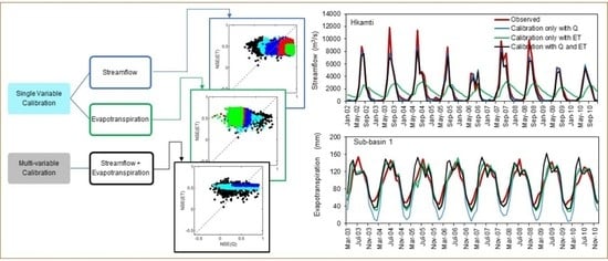
3.1.1. Calibration with a Single Variable

Note that all the model performance analysis presented in this study are based on monthly time series data. When adopting the single variable calibration approach, in general, model performance with respect to a variable with which it is calibrated against (e.g., streamflow) improves while the performance with respect to another variable (e.g., evapotranspiration) decreases (Figure 3). However, here the calibration with streamflow alone resulted in a reasonable performance in both streamflow and evapotranspiration on the monthly time series data. This is particularly true with respect to R2. For example, in the fifth iteration of Hkamti station, the NSE of streamflow varies between 0.74 and 0.94, whereas, NSE of evapotranspiration varies between 0.30 and 0.55. At the same station and same iteration, PBIAS of streamflow and evapotranspiration varies from −20.0% to −6.7%, and −5.2% to −15.6%, respectively, while R2 varies between 0.82 and 0.95 for streamflow, and between 0.8 and 0.85 for evapotranspiration. In contrast, calibration with evapotranspiration alone shows considerably low performance for streamflow. For the same example mentioned above, in the calibration with evapotranspiration alone, the NSE of streamflow ranges between −0.51 and 0.19, and NSE of evapotranspiration varies between 0.32 and 0.72. PBIAS values of streamflow and evapotranspiration vary between −60% to −12.9%, and −15.6% to −5.2%, respectively, while R2 varies between 0 and 0.31 for streamflow, and 0.8 and 0.85 for evapotranspiration (under the same conditions considered above).
However, when calibration is carried out at successive stations (starting at Hkamti, then Homalin, Kalewa, and ending at Monywa), the variability of performance reduces considerably for both variables (streamflow and evapotranspiration, Figure 3). This is not surprising because the upstream station is already calibrated for streamflow and evapotranspiration separately. In successive iterations, model simulations show approximately similar performance for both variables for calibration with evapotranspiration alone, but always with better values for evapotranspiration than for streamflow. However, in both calibration approaches, NSE is better for streamflow compared to evapotranspiration. For example, in the fifth iteration of Homalin, the NSE of streamflow varies from 0.91 to 0.95, and from 0.55 to 0.7 for single variable calibration with streamflow and evapotranspiration, respectively (Figure 3a). For the same iteration at the same station, weighted NSE values of evapotranspiration (from sub-basin 1 and 2) vary between 0.27 and 0.41, and between 0.67 and 0.72 in the two calibration approaches (streamflow alone and evapotranspiration alone). In contrast, streamflow shows higher bias: −15% to −11% and −28% to 21% for calibration with streamflow and evapotranspiration, respectively, whereas the bias of evapotranspiration changes between −14% to −9%, and between −5% to 4%, respectively (Figure 3b). However, R2 is greater than 0.77 for streamflow, and evapotranspiration in both calibration approaches (Figure 3c), implying that both variables preserve the temporal characteristics of observed data.
To assess the variation of the model performance belongs to best model simulation with respect to number of iteration, we analyzed the NSE as a representative model performance indicator of the best simulation in each iteration. In successive calibration iterations, an increase in the NSE of the calibration variable (either streamflow or evapotranspiration) is not always accompanied by a decline in the performance of the other variable (Figure 4a). For example, in the calibration with streamflow alone, the NSE of evapotranspiration increased when the NSE of streamflow also increased, and subsequently decreased in next iteration(s) at all stations but Kalewa station (Figure 4a). Similar results were also obtained in calibration with evapotranspiration alone (Figure 4b). This may be because different parameter combinations also could simultaneously increase the performances of both variables.

3.1.2. Calibration with Multiple-variables

In the multivariable calibration approach using streamflow and GLEAM ET, successive iterations improve the performance of evapotranspiration predictions compared to that of streamflow at all stations except the Hkamti station (Figure 5). For example, in the final iteration at Homalin, Kalewa, and Monywa, NSE values of streamflow vary between 0.86 and 0.92, 0.92 and 0.96, and 0.95 and 0.97, respectively. During the same simulation, the NSE values of evapotranspiration for the same stations vary between 0.46 to 0.66, 0.53 to 0.63, and 0.63 to 0.67, respectively (Figure 5a). In addition, PBIAS values of evapotranspiration vary between −6% and +7%, indicating under and over-estimations of evapotranspiration in all three above mentioned stations. However, model results always underestimated streamflow at all but the Monywa station (Figure 5b). With respect to R2, model calibrations show good performances (>0.77) for both streamflow and evapotranspiration at all the stations (Figure 5c). This behavior implies that simulated streamflow and evapotranspiration adequately capture the temporal variability in the observed data. Compared to single variable calibration, multivariable calibration also reduced biases in both streamflow and evapotranspiration.
In the best performed simulation in every successive iterations of multivariable calibration, the NSE of streamflow shows an increase in most of the cases, whereas that of evapotranspiration shows a reduction (Figure 4c). However, these decreases are small (e.g., from 0.62 to 0.61 at Kalewa station, and from 0.68 to 0.64 at Monywa station). In multivariable calibration, NSEs of evapotranspiration reduce at all but Kalewa station for every successive iteration (Figure 4c). Performance of streamflow does not always increase with the reduction of evapotranspiration performances. For example, at Homalin station, NSE of streamflow increases from 0.89 to 0.92 in the second iteration and reached 0.91 by the third iteration. Thus, a clear pattern in the performance of individual variables is not identified.

3.2. Model Perfroamnce with ‘Best Parameter Set’

When considering the best performing simulation in the last iteration for both single variable calibrations, results with streamflow alone show better performance in dry seasons (i.e., during low flows) than in monsoon seasons (high flows) (Figure 6a). Notably, the flows at Hkamti and Homalin are under estimated during high flow periods (June to August). This mismatch in high flows may be due to the poor spatial representation of rainfall over sub-basins. Model calibration with evapotranspiration alone under-estimates high flows and over-estimates the low flows at all stations for the entire simulation period.
When the calibration with evapotranspiration alone is considered, GLEAM ET and simulated ET show a well–matched seasonal variation of evapotranspiration in all the sub-basins (Figure 6b). However, in terms of magnitude or bias, model estimated ET is lower than the GLEAM ET during the dry period (December to February). In contrast, the model estimated ET is higher than GLEAM ET in sub-basins 6, 8, and 9 during the monsoon period. The calibration with streamflow alone under-estimates evapotranspiration in all sub-basins during the dry period, and over-estimates the same during the monsoon period particularly in sub-basins 1, 6, 8, and 9. Overall, calibration with streamflow alone appears to be capable of reproducing the observed evapotranspiration (in this case the GLEAM ET) at an acceptable level.
In multivariable calibration, simulated streamflow shows similar results obtained from calibration with streamflow alone (Figure 6a). However, high flows (during July to August) are less than the same resulted in calibration with streamflow alone. High flows are further underestimated in multivariable calibration. In contrast, simulated evapotranspiration at basin-level shows reasonably good performance similar to results obtained from calibration only with evapotranspiration (Figure 6b). Therefore, multivariable calibration shows reasonable estimations for both variables (i.e., streamflow and evapotranspiration).
Model performances corresponding to the best simulation at each of the station are presented in Table 1. Overall, in each performance indicator of streamflow, there is no significant difference among four stations. Among all sub-basins, the least accurate performances of evapotranspiration are for sub-basin 6, 8 and 9. These results imply that multivariable calibration is able to reproduce the observed streamflows better than evapotranspiration. However, model simulations produced a reasonably good estimation of evapotranspiration as well.
In general, the multivariable calibration with streamflow and GLEAM ET showed reasonably good streamflow estimations (NSE > 0.85). However, understandably, that calibration does not result in producing better streamflow performance than the results obtained from single variable calibration with streamflow only (Figure 4c, Figure 6a and Table 1). On the other hand, this multivariable calibration showed still sounds better for evapotranspiration as that from the single variable calibration with evapotranspiration only and better than the single variable calibration with streamflow only (Figure 6b).

3.3. Model Perfroamnce with ‘Good Parameter Sets’

Figure 7 presents the selected five global parameters (CN2, GW_DELAY, ALPHA_BF (Base flow Alpha Factor), SOL_AWC (Available Water Capacity in the Soil layer), and ESCO, details of parameters are in Table S1 in Supplementary Materials) and corresponding model performance for the last iteration of Hkamti station taking as an example station to discuss the variation of model performances with ‘good parameter set’.
In single variable calibration, four parameters show high variability for calibration with streamflow than with evapotranspiration, only ALPHA_BF shows high variability for calibration with evapotranspiration. Among these five parameters, CN2, GW_DELAY and ALPHA_BF are more sensitive to streamflow, whereas SOL_AWC and ESCO are more sensitive to evapotranspiration. In contrast, model performances show low variability except for performances of streamflow under calibration only with evapotranspiration (Figure 7). This implies that a range of parameter sets (100 sets considered here) can produce similar model performances of streamflow and evapotranspiration when those variables are calibrated separately. Therefore, these parameter ranges are very likely to show a similar level of performance with a dataset not used in calibration (i.e., validation dataset), unless inter/ intra-annual variability of the new dataset is considerably higher than calibration dataset.
In multivariable calibration, all the selected five global parameters show high variabilities (based on 100 ‘good parameter sets’ considered) compared to the variabilities associated with the single-variable calibration (Figure 7). These best performed simulations have resulted from different combinations of calibration parameter sets (100 ‘good parameter sets’), in which parameter value vary within a high range. Similar to single variable calibration, model performances (NSE, PBIAS, and R2) of streamflow and evapotranspiration vary within a narrow range (Figure 7), implying ‘good parameter sets’ can reproduce similar model results.

3.4. Parameter Sensitivity and Uncertainty

The most sensitive model parameters for streamflow and evapotranspiration were found to be different. Figure 8 shows the five most sensitive model parameters of each variable (streamflow and evapotranspiration) with respective MNSE values. GW_DELAY, RCHRG_DP (Deep aquifer Percolation fraction), ALPHA_BF, SLSOIL (Slope length for lateral subsurface flow), and LAT_TIME (Lateral flow travel time) are identified as the five most sensitive parameters for streamflow, whereas same parameters for evapotranspiration are SOL_BD (Moist bulk density of soil layer), SOL_Z (Depth from soil surface to bottom of layer), ESCO, EPCO, and SOL_AWC (refer Table S1 for definitions of parameters). Variations of MNSE for evapotranspiration-based calibration was found to be less than that for streamflow based calibration. In the multivariable calibration, weighted average MNSE values show less variation than individual streamflow and evapotranspiration calibrations. A considerable variation of parameter values are shown for ALPHA_BF and SOL_BD in evapotranspiration based model calibration. Results also indicate that, except SLSOL (subsurface lateral flow) and SOL_Z (depth of soil layer from surface), final parameter ranges in the last iteration of multivariable calibration are within the ranges of single variable calibration. The above two parameters directly correspond to changes in soil water balance.
Except for SLSOL, all the above identified sensitive parameters of streamflow are mostly related to the base flow (or groundwater flow) SLSOL parameter is related to the subsurface lateral flow. In model calibration with evapotranspiration alone, all the sensitive parameters are related to soil properties except for EPCO, which is the plant uptake compensation factor [61]. Parameter values resulting in a reasonable MNSE (> 0.5) are scattered within their initial ranges (for initial ranges, please refer to Table S1 in Supplementary Material). This scattered parameter values indicate that there are more than one combination of parameter values that can reproduce similar outputs.
For the multivariable calibration, each of the model parameter uncertainty range was examined in terms of normalized uncertainty scores (Equation (2)) that range from 0 to 100 (Figure 9). Uncertainty scores presented here were calculated from the last iteration of multivariable calibration. The analysis shows that uncertainty scores vary greatly among different parameters and stations for the same parameter. Parameters which are most sensitive to streamflow show higher uncertainty than the parameters sensitive to evapotranspiration except for SOL_BD. However, among the five most sensitive parameters for streamflow, SLSOIL and LAT_TIME show considerably less uncertainty at all the stations. In contrast, only ESCO, one of the most five sensitive parameters for evapotranspiration, shows considerably less uncertainty. Furthermore, uncertainty ranges for SOL_AWC are minimal at Homalin and Kalewa stations, whereas their maximum variations are found at Hkamti and Monywa stations.

4. Discussion

Results presented in this study are another application among a limited number of studies that have used GLEAM ET data to support hydrological model calibration in the data-scarce Chindwin River Basin in Myanmar. In general, under the three calibration approaches used, streamflow shows the best and worst performance in calibration only with streamflow and evapotranspiration, respectively, and vice versa in the calibration performance for evapotranspiration. Both variables show slightly lower performance in multivariable calibration than the individual calibrations with streamflow and evapotranspiration. In some of the sub-basins (e.g., sub-basins 2 to 4), simulated ET does not properly represent the GLEAM-ET during dry seasons (Figure 6b) under all three calibration approaches. In contrast, sub-basins 6, 8, and 9 overestimate ET during high flow periods (June to September) for the calibrations with streamflow and multivariable calibration. These differences can be attributed to the precipitation over the basins. Similar findings were obtained in a study on the Karkheh River Basin in Iran by Rientjes et al. (2013) [43]. They found that streamflow and ET obtain good performances when the variables are calibrated separately. However, for model calibration with both streamflow and ET, simulated ETs of most of the sub-basins show good agreement with SEBS-ET (satellite-based surface energy balance system – actual evapotranspiration). Immerzeel and Droogers (2008) [40] also could not find any improvement in streamflow simulation under the model calibration with satellite-based evapotranspiration from time series of MODIS images of the Upper Bhima catchment in south India. López et al. (2017) [42] also found that model calibration with GLEAM ET and soil moisture data shows a reasonable streamflow estimation (with NSE values varying from 0.5 to 0.75). However, better model performance was obtained when it was calibrated with in-situ streamflow data.
Tobin and Bennett (2017) [44] concluded that although there is no performance improvement in streamflow simulation, GLEAM ET data can be used to constrain the evapotranspiration parameters in the SWAT applications. They considered 16 major SWAT parameters, in which five are attributable to evapotranspiration (ESCO, EPCO, CANMX (Maximum canopy storage), GW_REVAP (Groundwater “revap” coefficient), and REVAPMN (Threshold water depth in shallow aquifer for “revap” or percolation to occur), refer to Table S1 for details). Here, ESCO and CANMX were identified as the most sensitive parameters for model calibration. Immerzeel and Droogers (2008) [40] found that actual ET is more sensitive to the groundwater (GW_REVAP) and meteorological (monthly rainfall increment––RFINC) parameters than soil (SOL_AWC) and land-use parameters (maximum plant leaf area index––BLAI). In our analysis, SOL_BD, SOL_Z, ESCO, EPCO, and SOL_AWC are found to be the most sensitive parameters for evapotranspiration. The analysis of ‘good parameter sets’ and resultant model performances imply that many combinations of model parameters can reproduce the streamflow and evapotranspiration comparable to same obtained from ‘the best parameter set’. Furthermore, Winsemius et al. (2009) [1] suggested that satellite-based ET and soil moisture information are required in hydrological model calibration to reduce parameter uncertainties and constrain model parameters within physically realistic ranges.
Even though we discussed only the parameter uncertainty, there are other sources of uncertainty in hydrological modelling, such as model input data, model structure, and observed data used for calibration [75,76]. Precipitation, the primary input data used in this analysis was derived from interpolated gauge data of six stations, which are not well distributed over the basin. Therefore, we believe that precipitation data contributes to prediction uncertainty. In terms of observed streamflow data, Harmel et al. (2009) [78] stated that the typical uncertainty in measured streamflow varies by ±7 − 23%. Di Baldassarre and Montanari (2009) [79] stated that the average error of measured streamflow data was 25.6% for the Po River, Italy. With respect to ET, the accuracy of remote sensing-based products may vary significantly over the different regions due to climatic variability, topography, and land cover [47]. For example, Trambauer et al. (2014) [3] have compared eight different ET products over the African continent and summarized that some products show good consistency among them in some areas and diverge in other areas of the continent. Another analysis by Tobin and Bennett (2017) [44] showed that simulated ET matches with GLEAM-TMPA (GLEAM - Tropical Rainfall Measurement (TRMM) Mission Multi-satellite Precipitation Analysis) better than GLEAM-CMORPH (GLEAM - Climate Prediction Center MORPHing technique). Therefore, these RS-based ET products may possess considerable biases. Thus, further information is required to analyze and discuss the uncertainty in model outputs.

5. Conclusions

This study evaluated the use of measured streamflow and RS-based ET data to calibrate a hydrological model of the Chindwin Basin, Myanmar. The model was developed with SWAT and two calibration approaches were tested: single variable and multiple variable calibration, and identified and discussed ‘good parameter sets’, which can produce similar or comparable results that obtained from ‘the best parameter set’. RS-based ET data used in the model calibration were obtained from the Global Land Evaporation: Amsterdam Model (GLEAM ET), and measured streamflow were obtained at four gauging stations in the basin.
In general, this study indicates that GLEAM ET data, together with streamflow data, offers good potential for hydrological model calibration in the study region as the simulation results show a good performance for streamflow (with an NSE > 0.85 on monthly time series), while maintaining a reasonable performance for evapotranspiration (with an NSE > 0.61). Moreover, the results of single variable calibration with GLEAM ET indicate that even in the absence of streamflow data (i.e., ungauged basin), the model would have produced streamflow NSE values of more than 0.69 for three out of four stations with PBIAS varying between −2.6% and −23%. The only exception to the above behavior was found at the Hkamti station with NSE of 0.16 and PBIAS of −22%. It is noted that the Hkamti station is the uppermost station of the four and hence its calibration is independent of the other three stations. In contrast, the other three stations (Homalin, Kalewa, and Monywa) are all downstream of Hkamti and in series. Thus, their calibration results are influenced by the calibration results of up-stream station(s).
Results also indicate that there can be many different sets of parameter values (‘good parameter sets’) can produce similar results, which can be obtained from ‘the best parameter set’. The analysis of calibration parameters suggests that the parameter sensitivity and their values change among different calibration set-ups, and uncertainty ranges of parameters may vary among both different parameters and stations.
This study provides valuable insights on hydrological modelling, in the context of using remote-sensing based and multiple data sources for model calibration, which are particularly useful for data poor basins. There is, however, room for further research on multivariable calibration in distributed hydrological modelling with the use of globally available datasets such as evapotranspiration, snow cover, and soil moisture data together with traditionally used streamflow data. Such a calibration approach could lead to better representation of hydrological responses of particularly, ungauged basins, as this approach would enable reasonable parameter estimation across the basin.

Supplementary Materials

The following are available online at https://www.mdpi.com/2072-4292/12/22/3768/s1. Table S1: Hydrological parameters used in model calibration.

Author Contributions

T.A.J.G.S. carried out the design, model simulations, analysis of results, and drafting the article. S.M. provided the guidance on methodology and comments on the manuscript. R.R. provided critical review for the manuscript. All authors have read and agreed to the published version of the manuscript.

Funding

This study is a part of TAJGS’s Ph.D research, which is supported by the EPP Myanmar project and Netherlands Fellowship Programme (NFP).

Acknowledgments

TAJGS is supported by the EPP Myanmar project and Netherlands Fellowship Programme (NFP). RR is supported by the AXA Research Fund and Deltares Strategic Research Programme “Coastal and Offshore Engineering.”. The SWAT simulations were carried out on the Dutch national e-infrastructure with the support of SURF Cooperative.

Conflicts of Interest

The authors declare no conflict of interest.

References

  1. Winsemius, H.C.; Schaefli, B.; Montanari, A.; Savenije, H.H.G. On the calibration of hydrological models in ungauged basins: A framework for integrating hard and soft hydrological information. Water Resour. Res. 2009, 45. [Google Scholar] [CrossRef] [Green Version]
  2. Sivapalan, M.; Takeuchi, K.; Franks, S.W.; Gupta, V.K.; Karambiri, H.; Lakshmi, V.; Liang, X.; McDonnell, J.J.; Mendiondo, E.M.; O’Conell, P.E.; et al. IAHS Decade on Predictions in Ungauged Basins (PUB), 2003–2012: Shaping an exciting future for the hydrological sciences. Hydrol. Sci. J. 2003, 48, 857–880. [Google Scholar] [CrossRef] [Green Version]
  3. Trambauer, P.; Dutra, E.; Maskey, S.; Werner, M.; Pappenberger, F.; Van Beek, L.P.H.; Uhlenbrook, S.; Park, S.; Section, W.R. Comparison of different evaporation estimates over the African continent. Hydrol. Earth Syst. Sci. 2014, 18, 193–212. [Google Scholar] [CrossRef] [Green Version]
  4. Shrestha, N.K.; Qamer, F.M.; Pedreros, D.; Murthy, M.S.R.; Wahid, S.M.; Shrestha, M. Evaluating the accuracy of Climate Hazard Group (CHG) satellite rainfall estimates for precipitation based drought monitoring in Koshi basin, Nepal. J. Hydrol. Reg. Stud. 2017, 13, 138–151. [Google Scholar] [CrossRef]
  5. Maskey, S. How can flood modelling advance in the “big data” age? J. Flood Risk Manag. 2019, 12, 10–11. [Google Scholar] [CrossRef] [Green Version]
  6. Courty, L.G.; Soriano-Monzalvo, J.C.; Pedrozo-Acuña, A. Evaluation of open-access global digital elevation models (AW3D30, SRTM, and ASTER) for flood modelling purposes. J. Flood Risk Manag. 2019, 12, 1–14. [Google Scholar] [CrossRef] [Green Version]
  7. Munyaneza, O.; Wali, U.G.; Uhlenbrook, S.; Maskey, S.; Mlotha, M.J. Water level monitoring using radar remote sensing data: Application to Lake Kivu, central Africa. Phys. Chem. Earth 2009, 34, 722–728. [Google Scholar] [CrossRef]
  8. Benveniste, J.; Berry, P. Monitoring River and Lake Levels from Space; ESA Bulletin: Noordwijk, The Netherlands, 2004; Volume 117, pp. 36–42. [Google Scholar]
  9. Huang, Q.; Long, D.; Du, M.; Zeng, C.; Li, X.; Hou, A.; Hong, Y. An improved approach to monitoring Brahmaputra River water levels using retracked altimetry data. Remote Sens. Environ. 2018, 211, 112–128. [Google Scholar] [CrossRef]
  10. Huss, M.; Bookhagen, B.; Huggel, C.; Jacobsen, D.; Bradley, R.; Clague, J.; Vuille, M.; Buytaert, W.; Cayan, D.; Greenwood, G.; et al. Towards mountains without permanent snow and ice. Earths Future 2017, 5, 418–435. [Google Scholar] [CrossRef]
  11. Bolch, T.; Kulkarni, A.; Kääb, A.; Huggel, C.; Paul, F.; Cogley, J.G.; Frey, H.; Kargel, J.S.; Fujita, K.; Scheel, M.; et al. The state and fate of himalayan glaciers. Science 2012, 336, 310–314. [Google Scholar] [CrossRef] [Green Version]
  12. Abrams, M.; Bailey, B.; Tsu, H.; Hato, M. The ASTER Global DEM. Photogramm. Eng. Remote Sens. 2010, 76, 344–348. [Google Scholar]
  13. Abrams, M.; Crippen, R.; Fujisada, H. ASTER Global Digital Elevation Model (GDEM) and ASTER Global Water Body Dataset (ASTWBD). Remote Sens. 2020, 12, 1156. [Google Scholar] [CrossRef] [Green Version]
  14. Jarvis, A.; Reuter, H.I.; Nelson, A.; Guevara, E. Hole-filled SRTM for the globe Version 4. The CGIAR-CSI SRTM 90m Database. Available online: http://srtm.csi.cgiar.org (accessed on 1 August 2016).
  15. Arino, O.; Perez, J.R.; Kalogirou, V.; Defourny, P.; Achard, F. Globcover 2009. In Proceedings of the ESA Living Planet Symposium, Bergen, Norway, 28 June–2 July 2010. [Google Scholar]
  16. Bartholomé, E.; Belward, A.S. GLC2000: A new approach to global land cover mapping from earth observation data. Int. J. Remote Sens. 2005, 26, 1959–1977. [Google Scholar] [CrossRef]
  17. Friedl, M.A.; Sulla-Menashe, D.; Tan, B.; Schneider, A.; Ramankutty, N.; Sibley, A.; Huang, X. MODIS Collection 5 global land cover: Algorithm refinements and characterization of new datasets. Remote Sens. Environ. 2010, 114, 168–182. [Google Scholar] [CrossRef]
  18. Beck, H.E.; Vergopolan, N.; Pan, M.; Levizzani, V.; van Dijk, A.I.J.M.; Weedon, G.; Brocca, L.; Pappenberger, F.; Huffman, G.J.; Wood, E.F. Global-scale evaluation of 22 precipitation datasets using gauge observations and hydrological modeling. Hydrol. Earth Syst. Sci. 2017, 21, 1–23. [Google Scholar] [CrossRef] [Green Version]
  19. Ashouri, H.; Hsu, K.L.; Sorooshian, S.; Braithwaite, D.K.; Knapp, K.R.; Cecil, L.D.; Nelson, B.R.; Prat, O.P. PERSIANN-CDR: Daily precipitation climate data record from multisatellite observations for hydrological and climate studies. Bull. Am. Meteorol. Soc. 2015, 96, 69–83. [Google Scholar] [CrossRef] [Green Version]
  20. Funk, C.; Peterson, P.; Landsfeld, M.; Pedreros, D.; Verdin, J.; Shukla, S.; Husak, G.; Rowland, J.; Harrison, L.; Hoell, A.; et al. The climate hazards infrared precipitation with stations—A new environmental record for monitoring extremes. Sci. Data 2015, 2, 150066. [Google Scholar] [CrossRef] [Green Version]
  21. Joyce, R.J.; Janowiak, J.E.; Arkin, P.A.; Xie, P. CMORPH: A Method that Produces Global Precipitation Estimates from Passive Microwave and Infrared Data at High Spatial and Temporal Resolution. J. Hydrometeorol. 2004, 5, 487–503. [Google Scholar] [CrossRef]
  22. Ushio, T.; Sasashige, K.; Kubota, T.; Shige, S.; Okamoto, K.; Aonashi, K.; Inoue, T.; Takahashi, N.; Iguchi, T.; Kachi, M.; et al. A kalman filter approach to the global satellite mapping of precipitation (GSMaP) from combined passive microwave and infrared radiometric data. J. Meteorol. Soc. Jpn. 2009, 87 A, 137–151. [Google Scholar] [CrossRef] [Green Version]
  23. Dee, D.P.; Uppala, S.M.; Simmons, A.J.; Berrisford, P.; Poli, P.; Kobayashi, S.; Andrae, U.; Balmaseda, M.A.; Balsamo, G.; Bauer, P.; et al. The ERA-Interim reanalysis: Configuration and performance of the data assimilation system. Q. J. R. Meteorol. Soc. 2011, 137, 553–597. [Google Scholar] [CrossRef]
  24. Hooker, J.; Duveiller, G.; Cescatti, A. Data descriptor: A global dataset of air temperature derived from satellite remote sensing and weather stations. Sci. Data 2018, 5, 1–11. [Google Scholar] [CrossRef] [PubMed] [Green Version]
  25. Bastiaanssen, W.G.M.; Cheema, M.J.M.; Immerzeel, W.W.; Miltenburg, I.J.; Pelgrum, H. Surface energy balance and actual evapotranspiration of the transboundary Indus Basin estimated from satellite measurements and the ETLook model. Water Resour. Res. 2012, 48, 1–16. [Google Scholar] [CrossRef] [Green Version]
  26. Miralles, D.G.; Holmes, T.R.H.; De Jeu, R.A.M.; Gash, J.H.; Meesters, A.G.C.A.; Dolman, A.J. Global land-surface evaporation estimated from satellite-based observations. Hydrol. Earth Syst. Sci. 2011, 15, 453–469. [Google Scholar] [CrossRef] [Green Version]
  27. Running, S.W.; Mu, Q.; Zhao, M. Alvaro Moreno User’s Guide MODIS Global Terrestrial Evapotranspiration (ET) Product (NASA MOD16A2/A3); NASA: Washington, DC, USA, 2017; p. 35.
  28. Njoku, E.G.; Jackson, T.J.; Lakshmi, V.; Chan, T.K.; Nghiem, S.V. Soil moisture retrieval from AMSR-E. IEEE Trans. Geosci. Remote Sens. 2003, 41, 215–228. [Google Scholar] [CrossRef]
  29. Dorigo, W.; Wagner, W.; Albergel, C.; Albrecht, F.; Balsamo, G.; Brocca, L.; Chung, D.; Ertl, M.; Forkel, M.; Gruber, A.; et al. ESA CCI Soil Moisture for improved Earth system understanding: State-of-the art and future directions. Remote Sens. Environ. 2017, 203, 185–215. [Google Scholar] [CrossRef]
  30. Landerer, F.W.; Swenson, S.C. Accuracy of scaled GRACE terrestrial water storage estimates. Water Resour. Res. 2012, 48, 1–11. [Google Scholar] [CrossRef]
  31. Rouholahnejad, E.; Abbaspour, K.C.; Srinivasan, R.; Bacu, V.; Lehmann, A. Water resources of the Black Sea Basin at high spatial and temporal resolution. Water Resour. Res. 2014, 50, 5866–5885. [Google Scholar] [CrossRef] [Green Version]
  32. Anderton, S.; Latron, J.; Gallart, F. Sensitivity analysis and multi-response, multi-criteria evaluation of a physically based distributed model. Hydrol. Process. 2002, 353, 333–353. [Google Scholar] [CrossRef]
  33. Beven, K.J.; Freer, J. Equifinality, data assimilation, and uncertainty estimation in mechanistic modelling of complex environmental systems using the GLUE methodology. J. Hydrol. 2001, 249, 11–29. [Google Scholar] [CrossRef]
  34. Beven, K.J. A Discussion of distributed hydrological modelling. In Distributed Hydrological Modelling; Abbott, J.C.R., Ed.; Kliwer Academic Publishers: New York, NY, USA, 1996; pp. 255–278. ISBN 978-0792340423. [Google Scholar]
  35. Fenicia, F.; Savenije, H.H.G.; Matgen, P.; Pfister, L. A comparison of alternative multiobjective calibration strategies for hydrological modeling. Water Resour. Res. 2007, 43, 1–16. [Google Scholar] [CrossRef]
  36. Beven, K.J. Rainfall-Runoff Modelling: The Primer, 2nd ed.; Willey-Blackwell: Hoboken, NJ, USA, 2012. [Google Scholar]
  37. Daggupati, P.; Yen, H.; White, M.J.; Srinivasan, R.; Arnold, J.G.; Keitzer, C.S.; Sowa, S.P. Impact of model development, calibration and validation decisions on hydrological simulations in West Lake Erie Basin. Hydrol. Process. 2015, 29, 5307–5320. [Google Scholar] [CrossRef]
  38. Molina-Navarro, E.; Andersen, H.E.; Nielsen, A.; Thodsen, H.; Trolle, D. The impact of the objective function in multi-site and multi-variable calibration of the SWAT model. Environ. Model. Softw. 2017, 93, 255–267. [Google Scholar] [CrossRef]
  39. Zhang, X.; Srinivasan, R.; Liew, M. Van Multi-site calibration of the SWAT model for hydrologic modeling. Trans. ASABE 2008, 51, 2039–2049. [Google Scholar] [CrossRef] [Green Version]
  40. Immerzeel, W.W.; Droogers, P. Calibration of a distributed hydrological model based on satellite evapotranspiration. J. Hydrol. 2008, 349, 411–424. [Google Scholar] [CrossRef]
  41. Franco, A.C.L.; Bonumá, N.B. Multi-variable SWAT model calibration with remotely sensed evapotranspiration and observed flow. Braz. J. Water Resour. 2017, 22, 1–14. [Google Scholar] [CrossRef] [Green Version]
  42. López, P.L.; Sutanudjaja, E.H.; Schellekens, J.; Sterk, G.; Bierkens, M.F.P. Calibration of a large-scale hydrological model using satellite-based soil moisture and evapotranspiration products. Hydrol. Earth Syst. Sci. 2017, 21, 3125–3144. [Google Scholar] [CrossRef] [Green Version]
  43. Rientjes, T.H.M.; Muthuwatta, L.P.; Bos, M.G.; Booij, M.J.; Bhatti, H.A. Multi-variable calibration of a semi-distributed hydrological model using streamflow data and satellite-based evapotranspiration. J. Hydrol. 2013, 505, 276–290. [Google Scholar] [CrossRef]
  44. Tobin, K.J.; Bennett, M.E. Constraining SWAT calibration with Remotely sensed Evapotranspiration data. J. Am. Water Resour. Assoc. 2017, 1–12. [Google Scholar] [CrossRef]
  45. Githui, F.; Selle, B.; Thayalakumaran, T. Recharge estimation using remotely sensed evapotranspiration in an irrigated catchment in southeast Australia. Hydrol. Process. 2012, 26, 1379–1389. [Google Scholar] [CrossRef]
  46. Zhang, Y.; Chiew, F.H.S.; Zhang, L.; Li, H. Use of remotely sensed actual evapotranspiration to improve rainfall–runoff modeling in Southeast Australia. J. Hydrometeorol. 2009, 10, 969–980. [Google Scholar] [CrossRef]
  47. Campo, L.; Caparrini, F.; Castelli, F. Use of multi-platform, multi-temporal remote-sensing data for calibration of a distributed hydrological model: An application in the Arno basin, Italy. Hydrol. Process. 2006, 20, 2693–2712. [Google Scholar] [CrossRef]
  48. Rajib, M.A.; Merwade, V.; Yu, Z. Multi-objective calibration of a hydrologic model using spatially distributed remotely sensed/in-situ soil moisture. J. Hydrol. 2016, 536, 192–207. [Google Scholar] [CrossRef] [Green Version]
  49. Li, Y.; Grimaldi, S.; Pauwels, V.R.N.; Walker, J.P. Hydrologic model calibration using remotely sensed soil moisture and discharge measurements: The impact on predictions at gauged and ungauged locations. J. Hydrol. 2018, 557, 897–909. [Google Scholar] [CrossRef]
  50. Kunnath-Poovakka, A.; Ryu, D.; Renzullo, L.J.; George, B. The efficacy of calibrating hydrologic model using remotely sensed evapotranspiration and soil moisture for streamflow prediction. J. Hydrol. 2016, 535, 509–524. [Google Scholar] [CrossRef]
  51. Finger, D.; Pellicciotti, F.; Konz, M.; Rimkus, S.; Burlando, P. The value of glacier mass balance, satellite snow cover images, and hourly discharge for improving the performance of a physically based distributed hydrological model. Water Resour. Res. 2011, 47, 1–14. [Google Scholar] [CrossRef]
  52. Finger, D.; Vis, M.; Huss, M.; Seibert, J. The value of multiple data set calibration versus model complexity for improving the performance of hydrological models in mountain catchments. Water Resour. Res. 2015, 51, 1939–1958. [Google Scholar] [CrossRef]
  53. Corbari, C.; Mancini, M. Calibration and Validation of a Distributed Energy—Water Balance Model Using Satellite Data of Land Surface Temperature and Ground Discharge Measurements. J. Hydrometeorol. 2013, 15, 376–392. [Google Scholar] [CrossRef]
  54. Pan, S.; Liu, L.; Bai, Z.; Xu, Y.P. Integration of remote sensing evapotranspiration into multi-objective calibration of distributed hydrology-soil-vegetation model (DHSVM) in a humid region of China. Water 2018, 10, 1841. [Google Scholar] [CrossRef] [Green Version]
  55. Ha, L.T.; Bastiaanssen, W.G.M.; van Griensven, A.; van Dijk, A.I.J.M.; Senay, G.B. Calibration of spatially distributed hydrological processes and model parameters in SWAT using remote sensing data and an auto-calibration procedure: A case study in a Vietnamese river basin. Water 2018, 10, 212. [Google Scholar] [CrossRef] [Green Version]
  56. FAO. The Digital Soil Map of the World (Version 3.6); FAO/UNESCO: Rome, Italy, 2003. [Google Scholar]
  57. Yuan, F.; Zhang, L.; Win, K.W.W.; Ren, L.; Zhao, C.; Zhu, Y.; Jiang, S.; Liu, Y. Assessment of GPM and TRMM multi-satellite precipitation products in streamflow simulations in a data sparse mountainous watershed in Myanmar. Remote Sens. 2017, 9, 302. [Google Scholar] [CrossRef] [Green Version]
  58. Sirisena, T.A.J.G.; Maskey, S.; Ranasinghe, R.; Babel, S. Effects of different precipitation inputs on streamflow simulation in the Irrawaddy River Basin, Myanmar. J. Hydrol. Reg. Stud. 2018, 19, 265–278. [Google Scholar] [CrossRef]
  59. Martens, B.; Miralles, D.G.; Lievens, H.; Van Der Schalie, R.; De Jeu, R.A.M.; Fernández-Prieto, D.; Beck, H.E.; Dorigo, W.A.; Verhoest, N.E.C. GLEAM v3: Satellite-based land evaporation and root-zone soil moisture. Geosci. Model Dev. 2017, 10, 1903–1925. [Google Scholar] [CrossRef] [Green Version]
  60. Arnold, J.G.; Kiniry, J.R.; Srinivasan, R.; Williams, J.R.; Haney, E.B.; Neitsch, S.L. Soil & Water Assessment Tool: Input/Output Documentation. Version 2012; Texas Water Resources Institute: College Station, TX, USA, 2012; p. 650. [Google Scholar]
  61. Neitsch, S.L.; Arnold, J.G.; Kiniry, J.R.; Williams, J.R. Soil and Water Assessment Tool Theoretical Documentation Version 2009; Texas Water Resources Institute: Temple, TX, USA, 2011. [Google Scholar]
  62. Abbaspour, K.C. SWAT-Calibration and Uncertainty Programs (CUP) 2015; Eawag: Swiss Federal Institute of Aquatic Science and Technology: Duebendorf, Switzerland, 2015. [Google Scholar]
  63. Vigiak, O.; Malagó, A.; Bouraoui, F.; Vanmaercke, M.; Poesen, J. Adapting SWAT hillslope erosion model to predict sediment concentrations and yields in large Basins. Sci. Total Environ. 2015, 538, 855–875. [Google Scholar] [CrossRef] [PubMed]
  64. Tuo, Y.; Duan, Z.; Disse, M.; Chiogna, G. Evaluation of precipitation input for SWAT modeling in Alpine catchment: A case study in the Adige river basin (Italy). Sci. Total Environ. 2016, 573, 66–82. [Google Scholar] [CrossRef] [PubMed] [Green Version]
  65. Nguyen, H.H.; Recknagel, F.; Meyer, W.; Frizenschaf, J.; Ying, H.; Gibbs, M.S. Comparison of the alternative models SOURCE and SWAT for predicting catchment stream flow, sediment and nutrient loads under the effect of land use changes. Sci. Total Environ. 2019, 662, 254–265. [Google Scholar] [CrossRef] [PubMed]
  66. Faramarzi, M.; Srinivasan, R.; Iravani, M.; Bladon, K.D.; Abbaspour, K.C.; Zehnder, A.J.B.; Goss, G.G. Setting up a hydrological model of Alberta: Data discrimination analyses prior to calibration. Environ. Model. Softw. 2015, 74, 48–65. [Google Scholar] [CrossRef]
  67. Dile, Y.T.; Karlberg, L.; Daggupati, P.; Srinivasan, R.; Wiberg, D.; Rockström, J. Assessing the implications of water harvesting intensification on upstream—Downstream ecosystem services: A case study in the Lake Tana basin. Sci. Total Environ. 2016, 542, 22–35. [Google Scholar] [CrossRef]
  68. Shrestha, N.K.; Wang, J. Predicting sediment yield and transport dynamics of a cold climate region watershed in changing climate. Sci. Total Environ. 2018, 625, 1030–1045. [Google Scholar] [CrossRef]
  69. Shrestha, B.; Babel, M.S.; Maskey, S.; Van Griensven, A.; Uhlenbrook, S.; Green, A.; Akkharath, I. Impact of climate change on sediment yield in the Mekong River basin: A case study of the Nam Ou basin, Lao PDR. Hydrol. Earth Syst. Sci. 2013, 17, 1–20. [Google Scholar] [CrossRef] [Green Version]
  70. Masih, I.; Maskey, S.; Uhlenbrook, S.; Smakhtin, V. Assessing the impact of areal precipitation input on streamflow simultions usimg the SWAT model. J. Am. Water Resour. Assoc. 2011, 47, 179–195. [Google Scholar] [CrossRef]
  71. Abbaspour, K.C.; Johnson, C.A.; van Genuchten, M.T. Estimating uncertain flow and transport parameters using a Sequential Uncertainty Fitting procedure. Vadose Zone J. 2004, 3, 1340–1352. [Google Scholar] [CrossRef]
  72. Rode, M.; Suhr, U.; Wriedt, G. Multi-objective calibration of a river water quality model-Information content of calibration data. Ecol. Modell. 2007, 204, 129–142. [Google Scholar] [CrossRef]
  73. Abbaspour, K.C.; Yang, J.; Maximov, I.; Siber, R.; Bogner, K.; Mieleitner, J.; Zobrist, J.; Srinivasan, R. Modelling hydrology and water quality in the pre-alpine/alpine Thur watershed using SWAT. J. Hydrol. 2007, 333, 413–430. [Google Scholar] [CrossRef]
  74. Rostamian, R.; Jaleh, A.; Afyuni, M.; Mousavi, S.F.; Heidarpour, M.; Jalalian, A.; Abbaspour, K.C. Application of a SWAT model for estimating runoff and sediment in two mountainous basins in central Iran. Hydrol. Sci. J. 2008, 53, 977–988. [Google Scholar] [CrossRef]
  75. Pechlivanidis, I.G.; Jackson, B.M.; Mcintyre, N.R.; Wheater, H.S. Catchment scale hydrological modelling: A review of model types, calibration approaches and uncertainty analysis methods in the context of recent developments in technology and applications. Glob. NEST 2011, 13, 193–214. [Google Scholar]
  76. Yang, J.; Reichert, P.; Abbaspour, K.C.; Xia, J.; Yang, H. Comparing uncertainty analysis techniques for a SWAT application to the Chaohe Basin in China. J. Hydrol. 2008, 358, 1–23. [Google Scholar] [CrossRef]
  77. Kumar, S.; Merwade, V. Impact of watershed subdivision and soil data resolution on swat model calibration and parameter uncertainty. J. Am. Water Resour. Assoc. 2009, 45, 1179–1196. [Google Scholar] [CrossRef]
  78. Harmel, R.D.; Smith, D.R.; King, K.W.; Slade, R.M. Estimating storm discharge and water quality data uncertainty: A software tool for monitoring and modeling applications. Environ. Model. Softw. 2009, 24, 832–842. [Google Scholar] [CrossRef]
  79. Di Baldassarre, G.; Montanari, A. Uncertainty in river discharge observations: A quantitative analysis. Hydrol. Earth Syst. Sci. 2009, 13, 913–921. [Google Scholar] [CrossRef] [Green Version]
Figure 1. Chindwin River Basin, Myanmar (a) location and topography, (b) land use (top) and soil type (bottom), and (c) climate. Temperature data for Mawlaik and Kalewa are not available for the same period.
Remotesensing 12 03768 g001
Figure 2. (a) Inter-annual variability of GLEAM ET data over the Chindwin Basin for the period of 2003–2010, and (b) average annual evapotranspiration of each sub-basin.
Remotesensing 12 03768 g002
Figure 3. Model performance of each iteration in single variable calibration (a) Nash–Sutcliffe Efficiency (NSE), (b) percentage of bias (PBIAS), and (c) coefficient of determination (R2). ‘Q’ means streamflow and ‘ET’ means evapotranspiration. Left and right columns respectively show the results of calibration with streamflow alone and evapotranspiration alone for each efficiency indicator. The names in the sub-plots refer to the streamflow gauging stations from up-stream to down-stream. Each station refers to the different sub-basins: Hkamti—1, Homalin—1 and 2, Kalewa—1 to 4, and Monywa—1 to 9. The indicators of evapotranspiration represent comparisons of area-weighted average evapotranspiration of simulated and observed data.
Remotesensing 12 03768 g003
Figure 4. NSE of the best simulation in each iteration performed at each station under (a) calibration only with streamflow (Q), (b) calibration only with ET, and (c) calibration with both streamflow and ET. The scales of two y-axes in each plot are not identical.
Remotesensing 12 03768 g004
Figure 5. Model performance of each iteration in the multivariable calibration (a) NSE (b) PBIAS (c) R2. Similar to Figure 3 performances of evapotranspiration are evaluated via area-weighted average evapotranspiration for each corresponding streamflow station.
Remotesensing 12 03768 g005
Figure 6. Comparison of simulated and observed (a) streamflow and (b) evapotranspiration for the best simulation of the last iteration for each single variable calibration approach for four stations and nine sub-basins.
Remotesensing 12 03768 g006aRemotesensing 12 03768 g006b
Figure 7. Box plots of selected global parameters of best 100 simulations for each calibration approach (single variable: Q and ET separately and multivariable: Q + ET) at Hkamti station (top panel) and the corresponding range of performance indicator values of streamflow (blue) and ET (red) (bottom panel). In each plot, the boxes are limited to 25th and 75th percentiles of sample and thick line shows the median value. Whiskers are extended to 1.5 times inter-quartile range to the top and bottom of the boxes.
Remotesensing 12 03768 g007
Figure 8. Parameter values or absolute changes versus objective function MNSE for each iteration with 2000 simulations for calibration with a single variable; blue dots represent calibration based on streamflow, red dots represent calibration based on evapotranspiration, and black dots for multivariable calibration. Y-axis is a MNSE value ranging from 0 to 1 and the X-axis represents the changes of parameter value or absolute change of a corresponding parameter. ‘v_’ denotes replacement of the existing parameter value (e.g., v_GW_DELAY.gw), ‘a_’ denotes adding a fix value to existing value (e.g., a_SOL_BD.sol). The first five parameters correspond to streamflow and the last five to evapotranspiration.
Remotesensing 12 03768 g008
Figure 9. Normalized uncertainty scores of selected parameters out of 22 parameters used. Each box plot contains parameter values corresponding to 2000 simulations for the last iteration of multivariable calibration.
Remotesensing 12 03768 g009
Table 1. Model performance for monthly streamflow and evapotranspiration of the Chindwin River Basin. Results represent the overall best model simulation in the last iteration of the multivariable calibration at each station and sub-basin. A: Model calibration with streamflow only. B: Model calibration with evapotranspiration only. C: Model calibration with both streamflow and evapotranspiration. The best statistical performance among the streamflow stations and among the evaporation at sub-basin levels indicates in bold for each calibration approach.
VariableStation/Sub-BasinNSEPBIAS %R2
ABCABCABC
StreamflowHkamti0.930.160.86−9.2−21.8−17.40.950.220.91
Homalin0.940.660.91−11.2−23.1−17.50.950.850.95
Kalewa0.970.620.96−3.5−16.2−8.50.970.830.97
Monywa0.980.700.971.4−3.7−1.70.980.800.97
EvaporationSub-basin 10.360.740.57−12.8−0.43.90.840.820.73
Sub-basin 2−0.080.550.26−16.9−9.1−13.90.870.850.88
Sub-basin 30.360.590.39−12.5−4.9−11.20.840.800.84
Sub-basin 40.270.300.32−13.53.1−11.50.860.770.86
Sub-basin 50.760.670.783.5−6.82.80.810.810.83
Sub-basin 6−0.610.09−0.4823.99.321.70.81 0.82 0.80
Sub-basin 70.720.800.795.3−7.82.30.740.860.80
Sub-basin 8−0.980.47−0.7337.3−2.934.30.650.680.66
Sub-basin 9−0.170.24−0.2028.0−14.230.30.470.440.50
Note: The best statistical performance among the streamflow stations and among the evapotranspiration at sub-basin levels indicated in bold.
Publisher’s Note: MDPI stays neutral with regard to jurisdictional claims in published maps and institutional affiliations.

