Article

Examining the Robustness of a Spatial Bootstrap Regional Approach for Radar-Based Hourly Precipitation Frequency Analysis

1
Department of Civil Engineering, University of Louisiana at Lafayette, Lafayette, LA 70503, USA
2
Department of Civil Engineering and Watershed Flood Center, University of Louisiana at Lafayette, Lafayette, LA 70503, USA
*
Author to whom correspondence should be addressed.
Currently address: Department of Civil and Environmental Engineering, University of Washington, Seattle, WA 98195, USA.
Remote Sens. 2020, 12(22), 3767; https://doi.org/10.3390/rs12223767
Submission received: 30 September 2020 / Revised: 6 November 2020 / Accepted: 10 November 2020 / Published: 16 November 2020
(This article belongs to the Special Issue Remote Sensing of Precipitation: Part II)

Abstract

:
Radar-based Quantitative Precipitation Estimates (QPE) provide rainfall products with high temporal and spatial resolutions as opposed to sparse observations from rain gauges. Radar-based QPE’s have been widely used in many hydrological and meteorological applications; however, using these high-resolution products in the development of Precipitation Frequency Estimates (PFE) is impeded by their typically short-record availability. The current study evaluates the robustness of a spatial bootstrap regional approach, in comparison to a pixel-based (i.e., at site) approach, to derive PFEs using hourly radar-based multi-sensor precipitation estimation (MPE) product over the state of Louisiana in the US. The spatial bootstrap sampling technique augments the local pixel sample by incorporating rainfall data from surrounding pixels with decreasing importance when distance increases. We modeled extreme hourly rainfall data based on annual maximum series (AMS) using the generalized extreme value statistical distribution. The results showed a reduction in the uncertainty bounds of the PFEs when using the regional spatial bootstrap approach compared to the pixel-based estimation, with an average reduction of 10% and 2% in the 2- and 5-year return periods, respectively. Using gauge-based PFE’s as a reference, the spatial bootstrap regional approach outperforms the pixel-based approach in terms of robustness to outliers identified in the radar-based AMS of some pixels. However, the systematic bias inherent to radar-based QPE especially for extreme rainfall cases, appear to cause considerable underestimation in PFEs in both the pixel-based and the regional approaches.

1. Introduction

Rainfall plays a critical role in the earth’s water and energy cycle over a wide range of spatiotemporal scales. Therefore, accurate quantitative estimation of rainfall is an important input for engineering design applications where Precipitation Frequency Estimates (PFE) are highly sought [1]. The purpose of a precipitation frequency analysis is to determine the frequency at which certain intensities or depths of precipitation are expected to occur. Probabilistic modeling and statistical analysis techniques of extreme rainfall are used to provide PFE information and characterize the relationships between three important precipitation variables: intensity (or depth), duration, and frequency [2]. Such relationships are usually referred to as Intensity-Duration-Frequency (IDF) or Depth-Duration-Frequency (DDF) curves. Statistics derived from IDF or DDF curves are typically used to develop design storms, which are then used as an input for a variety of engineering applications such as design of dams, levees, reservoirs, and urban sewer systems [3].
Precipitation frequencies are typically estimated using sparse gauge observations. The evolution of weather radars allows the spatially continuous estimation of rainfall at small temporal sampling intervals, thereby filling the observational gap of rain gauges in space and time. Radar does not measure surface rainfall directly; instead, it measures the backscattered power from the hydrometeors aloft and the received power is then converted into rainfall estimates with inherent errors. The availability of NEXRAD Quantitative Precipitation Estimates (QPE) in high temporal and spatial resolutions covering the United States (US) has motivated researchers to study the applicability of the radar-based QPE in deriving precipitation frequencies [4,5,6,7,8]. For instance, Overeem, et al. [8] used radar data covering the entire land surface of the Netherlands for a 10-year period (1998–2008) to derive radar-based areal reduction factors (ARFs), which were found comparable to those based on high-density rain gauge networks and thus concluded that radar data, after careful quality control, are suitable to estimate extreme areal rainfall depths.
For sites that sufficiently have long records with respect to the return period of the extreme precipitation quantile of interest, at-site frequency analysis can be an adequate approach. However, for un-gauged sites, or for sites with historical records that are too short to make a reliable prediction of extreme quantiles, data augmentation from neighboring sites is needed. Thus, two main approaches for the frequency analysis have been discussed in the literature. The first is an at-site estimation approach, which simply uses data at each station, while the second method is a regional estimation approach that makes use of observations from gauges sharing a homogenous region with similar climatological and physical characteristics [9,10,11,12,13,14]. Svensson & Jones [13] reviewed the different estimation methods of rainfall frequency analysis in nine countries and reported that, while each country’s method is different, most of them use some form of regionalization to transfer information from surrounding sites to the target location. A regionalization method combines a local estimate of an index variable (typically the mean or median annual maximum rainfall) with a regionally derived growth curve to obtain a design rainfall estimate. Naghavi & Yu [15] applied a regional frequency approach to precipitation data in Louisiana using Annual Maximum Series (AMS) extracted from 25 synthesized stations with long periods of record. The results showed that the regional approach can substantially reduce the relative root-mean-square error (RRMSE) and the relative bias (RBIAS) in precipitation quantile prediction.
Although radar QPE can provide site (pixel)-specific PFEs with a high spatial resolution, regionalization techniques could be advantageous to reduce the sampling variability in the radar PFEs [4,6,16]. Eldardiry et al. [16] tested three regional estimation procedures and indicated lower uncertainty bounds associated with regional approaches compared to pixel-based PFEs. However, they also reported on the effect of the relatively short radar records on the uncertainty associated with the radar-based quantiles. Using QPE data during 1993–2000 over the Arkansas-Red Basin River Forecast Center (ABRFC), Durrans et al. [4] concluded that data heterogeneities and the temporally-limited data records are major factors that hinder the development of depth-area relationships using radar-rainfall data.
In this study, we assess the robustness of a probability weighted regional spatial bootstrap approach to estimate precipitation frequencies using radar data. This method was proposed by Uboldi et al. [17] as a resampling approach for estimation of parameters of rainfall annual maximum series statistical distribution. Using the regional spatial bootstrap technique, we investigate two main issues that impact the use of radar-based QPE in deriving precipitation frequency estimates: (1) the typically short historical records of radar-based QPEs; and (2) the effect of outliers in precipitation maxima series that could possibly cause unrealistic spatial gradients in IDF relations. We assess the utility of the spatial bootstrap approach in alleviating such limitations and compare the PFEs from the regional bootstrap approach against estimates derived using an at-site (pixel-based) method and PFEs reported in a US gauge-based Precipitation-Frequency Atlas [18]. The study is performed using radar-based QPEs over the state of Louisiana, USA.

2. Datasets and Methods

2.1. Radar MPE Dataset

NEXRAD (Next-Generation Radar) is a network of more than 160 high-resolution S-band Doppler weather radars operated by the US National Weather Service (NWS). The NEXRAD system provides high-quality, high-resolution precipitation estimates for a wide range of hydro-meteorological applications [19]. Starting in 2002, the NWS implemented a processing algorithm called the Multisensor Precipitation Estimator (MPE) [1], which is currently used at the NWS River Forecast Centers (RFC) to produce a set of regional rainfall products using single- or multi-sensor analysis techniques. However, radar-based estimates can be highly uncertain due to a number of sampling and algorithm factors e.g., [20,21,22]. Therefore, the MPE algorithm applies bias-correction and co-Kriging optimal merging techniques using gauge reports [1,23].
The specific radar product used in this study is the operational product produced at the NWS Lower Mississippi River Forecast Center (LMRFC). This product is developed using the MPE algorithm, but also benefits from manual adjustments by human forecasters [22,24,25]. The MPE product has an hourly resolution and projected spatially using the Hydrologic Rainfall Analysis Project (HRAP) grid [26], with an approximate pixel size of 4-km x 4-km. The domain of the current study covers the entire state of Louisiana in the south-central US. With proximity to the Gulf of Mexico, different synoptic weather patterns are responsible for extreme events over Louisiana, including tropical storms, fronts, and convective air mass thunderstorms [27]. For the purposes of this study, the radar pixels covering Louisiana were extracted from the full LMRFC MPE product, resulting in a matrix with a total number of pixels of (180 × 140). The dataset comprises a total of 11 years covering the period of 2002–2012. To perform a precipitation frequency analysis, the annual maximum series (AMS) were extracted over each of the (180 × 140) radar pixels, resulting in a sample composed of a spatial field of 11 maxima representing the maximum hourly rainfall during 2002–2012 at each 4-km × 4-km pixel within the study domain.

2.2. Estimation of Parameters of AMS Probability Distribution

Various distributions have been proposed for modeling extreme events, including the Generalized Extreme Value distribution (GEV), Generalized Pareto distribution (GP), gamma distribution, lognormal distribution, among others. The GEV distribution was recommended for flood frequency analysis in the United Kingdom (UK) Flood Studies Report [28]. According to the gauge-based Precipitation-Frequency Atlas of the US National Oceanic and Atmospheric Administration (NOAA) Atlas 14 [18], the GEV distribution provided an acceptable fit to data more frequently than any other distribution and was chosen to model the annual maximum series of all the stations covering the US southeastern states (Alabama, Arkansas, Florida, Georgia, Louisiana and Mississippi). These conclusions were obtained using a goodness-of-fit test based on L-moment statistics for 3-parameter distributions along with the results of χ2 and Kolmogorov-Smirnov tests and visual inspection of probability plots. Naghavi & Yu [15] examined six different distributions for extreme precipitation over Louisiana and concluded that GEV distribution outperforms other distributions. Therefore, the GEV will be adopted in the current study to represent the AMS. The GEV distribution is a three-parameter distribution developed within the extreme value theory and combines three different models: Gumbel, Frechet and Weibull distributions, which are often referred to as Types (I), (II), and (III) distributions, respectively. The probability density function of the GEV distribution, in terms of its three parameters: Location (α), Scale (β), and Shape (κ ≠ 0), can be formulated as follows:
f X x = 1 β [ 1 κ β x α ] 1 / κ 1 F X x
In this study, the method of linear moments is used for the estimation of the GEV distribution parameters. The method of L-moments offers several advantages over other methods (e.g., method of moments, and method of maximum likelihood), especially in the cases of small sample sizes [29,30]. The L-moment estimators for the GEV distribution parameters are given as follows:
κ ^   = 7.8590 c + 2.9554 c 2
c = 2 3 +   τ ^   3 log 2 log 3
α ^   =   λ ^   1   β ^     κ ^   1 Γ 1 +   κ ^  
β ^   =   λ ^   2   κ ^   1 2   κ ^   Γ 1 +   κ ^  
where τ3 (or L-skewness) is the ratio of the third and second L-moment (a measure of skewness), λ1 is the first L-moment (measure of distribution mean), and λ2 is the second L-moment (measure of the scale or dispersion). Accordingly, the quantiles corresponding to different return periods, T, (e.g., T = 5, 10, 50, 100 years) can be estimated as follows:
x q = α +   β ^     κ ^   [ 1 ln q ) κ ^
where q is the cumulative probability of interest that can be related to the return period T as q = 1 1 T .

2.3. At-Site and Regional PFE Estimation Methods

Two estimation approaches for the frequency analysis of extreme precipitation, at-site (or pixel-based) and regional, are applied using the radar product and compared to each other. Uncertainties due to sampling effects are quantified in terms of confidence bounds using the difference between the 95th and 5th percentiles. The results of each method will also be compared to the corresponding gauge-based estimates that are reported in the NOAA Atlas 14 PFEs [18].

2.3.1. Pixel-Based Method

This approach is analogous to at-site frequency analysis of extreme precipitation from rain gauge stations, which was originally applied by the NWS to establish the rainfall frequency isohyetal maps for the US [31]. Treating each 4-km × 4-km HRAP radar pixel as a single station, this is equivalent to considering the domain of study as a dense network of stations that are located 4 km apart from each other. At each pixel, the AMS sample of hourly precipitation, constructed from the 11-year radar dataset, is fitted to the GEV model and the parameters of the distribution are estimated at each pixel using the L-moment method. The quantiles corresponding to different return periods (e.g., 5, 10, 25, 50, 100) can then be estimated at each pixel using the GEV parameters. Confidence intervals for the pixel-based parameter and quantile estimates are constructed using the classical scalar bootstrap procedure suggested by Efron [32]. The bootstrap procedure is used to generate a large number of samples (500 in our case) for each individual pixel.

2.3.2. Regional Spatial Bootstrap Method

This is a probability weighted regional method that was originally proposed by Uboldi et al. [17] as a resampling approach for estimation of parameters of the AMS distribution. This technique is based on the generation of a regional sample at any desired location by taking into account data observed at surrounding stations but with decreasing importance when distance increases. Thus, the probability of contribution of a certain station decreases as it goes far away from the desired location. The probability of sampling also takes into consideration the length of the time series at each station, and as such, the possibility of oversampling can be avoided, and the use of short time series is enabled. This method is basically a spatial bootstrap technique in which a regional sample is generated repeatedly from the surrounding locations (pixels in the case of radar data) based on the randomness produced from the probability of data extracting. The procedure of this approach involves formation of a homogenous region, construction of a regional sample, estimation of statistical distribution parameters, repeating the regional sampling and parameter estimation several times as in any bootstrap technique, and finally obtaining a distribution of estimates for each parameter.
The regional sample of size (N) is constructed by extracting (N) observations randomly from all of the available data (M) in a homogenous region. The probability of extraction of each observation is assumed to be proportional to a prescribed Gaussian function (γm) of the distance between the station at the desired location (X) and any other station (Km). Using spatially continuous radar observations (pixel resolution of ~4 km in the current study), the spatial bootstrap methodology is implemented as follows. For each pixel at a desired location X, and by prescribing distance-dependent extraction probabilities, observations from nearby pixels are selected more often than observations from pixels located far away. The probability of extraction of the mth observation located at a pixel (Km) is given by the following relation:
γ m = exp 1 2 d h X , k m D h 2 . exp 1 2 d v X , k m D v 2
where dh(X, Km) and dv(X, Km) are the horizontal and vertical distance between pixel Km and the pixel at the desired location (X). The Dh and Dv are scale parameters that are selected to impose some degree of smoothing and were chosen in this study to be equal to the standard deviation of the available distances between (X) and (Km).
Normalized by the sum of probabilities of all the observations (M), the probability of extraction of each observation from N set of available observations can be obtained as follows:
γ ¯   m = γ m Γ ,   Γ = m = 1 M γ m
By sorting the (M) observations in a descending order according to their probability of extraction ( γ ¯   m ) and assigning each observation a number (m) from 1 to M, a series of sequential ordered dataset is obtained. The cumulative normalized probability of extraction ( γ ¯   m ) of each observation ranges between (0, 1) and the probability of extraction of this cumulative probability is assumed to be uniformly distributed, i.e., ( γ ¯   m )~U (0,1). A continuous random variable (ρ) is then used to implement a random number generator for a discrete random variable (m) with any prescribed (non-uniform) probability distribution on positive integers up to a generic M. By generating a random number (ρ), the corresponding cumulative probability ( γ ¯   m ) is equal to the generated random number (ρ) and realization number (m) is equal to the first observation that has cumulative probability greater than or equal to the generated probability (ρ).
The spatial bootstrap regional approach requires the formation of a homogenous region surrounding each pixel, from which a regional sample can be constructed. The identification of homogenous regions is a non-trivial step in the regional frequency analysis, and it may require subjective judgement [33]. A homogenous region is the area including a group of sites, or pixels as in the case of radar fields, that share similar physical characteristics. The advantages of working with a homogeneous region is that the historical data available within the region can be pooled to get an efficient estimate of parameters and hence a more robust quantile estimate [34]. Hosking & Wallis [33] strongly preferred to base the formation of homogenous regions on site characteristics (e.g., by using geographical delineation, cluster analysis, or principle components analysis) and to use the at-site statistics only in subsequent testing of the homogeneity of the proposed set of regions. Conventional regionalization techniques identify a fixed set of sites to form a contiguous region, resulting in fixed-boundary regions without smooth transitions.
Burn [10] presented the Region of Influence (ROI) approach for defining homogenous region, in which every site can have a potentially unique set of gauging stations to be used in the estimation of at-site extremes. The ROI technique is recommended as it avoids the transition problems across fixed boundaries by introducing smooth change in the estimates across the boundaries of the regions. The selection of the radius of influence is a trade-off problem, in which a large radius R will increase the number of sites included in each ROI, but at the expense of the homogeneity of the set of sites included. Conversely, a small radius R will ensure the homogeneity of the sites included, but the information transfer will be decreased due to the smaller number of sites. In this study, the ROI approach is applied by using a square window with an area equivalent to (2R + 1)2 bounding the pixel of interest (R is the radius of influence and is used here to refer to the number of pixels considered in the horizontal or vertical directions between the central pixel and the edge of the square window). The window forms a homogenous region and constructs the regional sample for the target pixel (central pixel) using the pixels lying inside this window.
Since the choice of a homogenous region, or the window size, should be based on climatic and physical characteristics, the US Climate Divisions are used in this study to provide an indication for the reasonable range of the radius of influence (R). Louisiana has nine Climate Divisions (Figure 1) and the average area of each climate division is approximately covering a window with side length of about 31 pixels, which corresponds to R = 15 pixels.
Therefore, we chose R = 15 as a threshold for identifying the homogenous regions to estimate PFE. In this study, we tested different square windows ranging from R = 3 pixels to R = 15 pixels (results are only shown for R = 5 and 10) to study the effect of the region size on the uncertainty of the estimates. For example, increasing the window size to 21 × 21, by setting R = 10 pixels, allows for many more pixels (M = 441 × 11; 441 pixels with AMS of 11 observations in each pixel) to be included in the region of each target pixel. The scale parameters in Equation (7), i.e., Dh and Dv, are chosen to be approximately equal to the standard deviation of each radius of influence (for R = 5, Dh = Dv = 1 pixel and for R = 10, Dh = Dv = 3 pixels). The regional sample size is chosen to be the same as the actual number of years available in the radar dataset, i.e., N = 11 (sampled out of the M observations).
In order to reduce the likelihood of extracting annual maxima that might come from the same event, a constraint is added in such a way that the gap in the time stamp of any two annual maxima extracted from two different pixels must be greater than 6 h. This criterion is evaluated using the Julian Date in which the 6 h represent 0.25 day. For instance, if the extracted annual maximum occurs in a certain Julian Date (JD), then any new annual maximum must have a new Julian Date greater than (JD + 0.25) or smaller than (JD − 0.25). This restriction might not be necessary in the case of gauge-based PFE analysis since the gauges are separated with relatively large distances, and therefore it is less probable to have annual series in two gauges that share exactly the same events. On the other hand, the application of this conditioned extracted annual maxima is critical to the radar-based annual maxima, since they are provided on a uniform grid with high spatial resolution (4-km × 4-km in our dataset).

3. Results

3.1. Characterization of Annual Maxima

Radar precipitation estimates provide new possibilities to investigate the climatology of extreme rainfall at high spatial resolutions and over large areas [7]. Louisiana is considered one of the wettest of the contiguous 48 US states with extreme events that are generated by various rainfall mechanisms. Extreme events in the Southeastern US are typically generated from different synoptic weather patterns, for example, tropical storms, fronts, and convective airmass thunderstorms [27]. Figure 1a shows the Mean Annual Maxima (MAM) rainfall depth for each pixel in the domain of the study area. Most of the maxima are in the range between 20 mm and 100 mm with a significant spatial increase towards the gulf coastal zone. Figure 1b depicts the spatial distribution of average month of occurrence for annual maximum rainfall and shows dominance of the summer season (June—July—August) throughout most of the state. These results agree with Maddox et al. [35] who concluded that most of the extreme events that cause flash floods are of convective nature with the predominance of events in the warm season (April-September). The diurnal distribution of the annual maxima is illustrated by the average 6-h of annual maxima occurrence (Figure 1c). Most of the annual maxima occurred between 18:00 UTC and 00:00 UTC, while fewer number of events occurred in the two intervals (00:00 UTC–06:00 UTC) and (12:00 UTC–18:00 UTC).

3.2. Radar-Based PFE using Regional Sptail Bootstrap

Before presenting the results of PFEs using the spatial bootstrap technique, we first examine the traditional at-site method (pixel-based in case of using radar datasets). The pixel-based estimation procedure described in Section 2.3.1 was applied to the radar dataset to estimate the GEV distributional parameters and the corresponding PFE for different return periods ranging from 2 to 100 years. Confidence intervals for the estimated parameters and PFEs were also derived using classic scalar bootstrap sampling at each pixel. The parameters and PFEs for each pixel are represented using the mean of the 500 runs of bootstrap. The difference between the lower 5% and upper 95% quantiles of the bootstrap samples are used to quantify the uncertainty in the estimates. The confidence intervals are calculated using a non-parametric method, in which a probability is initially assigned to the sorted values of the sample ((0.5/n), (1.5/n), ([n—0.5]/n)), where n is the sample size (n = 500 bootstrap runs). The quantiles are then computed by setting the probability to be equal to the confidence limit required, e.g., 0.95, 0.90, 0.05, or 0.1. The first and last value in the bootstrap sample are assigned to the quantiles for probabilities less than (0.5/n) and greater than ([n—0.5]/n), respectively. Figure 2 and Figure 3 show the GEV parameters estimated at each pixel using the pixel-based and regional spatial bootstrap methods, respectively, over the domain of study covering Louisiana.
The shape parameter, estimated from the average of 500 bootstrap runs, varies between positive and negative values mostly between [−0.5, 0.5]. The 5% and 95% confidence of the shape parameter have values below −0.5 and above 1 due to the sampling variability. The scale parameter, in most pixels, falls in the range between 5 and 20, with some subtle spatial patterns. The location parameter has noticeable spatial gradients similar to those of the MAM (Figure 1a) where the location parameter increases from north to the south and as we get closer to the Gulf boundary. The sampling effect on both of the scale and location parameters is evident in the 5% and 95% confidence limits. The corresponding PFEs are displayed for two representative return periods of 2 and 10 years (Figure 4 and Figure 5). The PFE results show significant variability in space with clear gradients from north to south. The uncertainty associated with these estimates is fairly large, especially for large return periods, e.g., 50 and 100 years (figures not shown). The spatial maps also show clear signs of irregularities and inconsistency in the spatial variability of the estimated quantiles, which are mostly noticed for large return periods.
The confidence limits are estimated using the spatial bootstrap technique for 500 runs using a moving window of 11 × 11 pixels (R = 5). Compared to the pixel-based approach, the results suggest that the spatial bootstrap approach reduced the estimated parameters and resulted in narrower confidence intervals. For instance, the mean shape parameters, in most of the pixels, went down to the range [−0.2, 0.2] with a noticeable reduction in the width of the uncertainty bounds. The reduction in the dispersion of the estimated parameters is attributed to the gain from the repeated sampling from the surrounding pixels, which is the main advantage of a regional estimation as opposed to using information available at each pixel only. Sampling from a homogenous region resulted in smoother fields of the GEV parameters with less sampling variability. Because of the short record available in each pixel, only 11 years, the pixel-based estimation varies considerably from one pixel to another, which was circumvented when using the regional spatial bootstrap estimation with the moving window at each pixel. Increasing the size of the moving window to (21 × 21) or R = 10 pixels resulted in lower variability and more smoothness for the estimates transition between the pixels (figure not shown), but possibly at the expense of losing details in the spatial patterns.
Figure 4 and Figure 5 display the PFEs using the GEV distribution parameters for return periods of 2 and 10 years. Improvements in the smoothness of the different PFEs can obviously be seen when using the spatial bootstrap approach over the pixel-based approach. The smoothness in the PFEs patterns by the spatial bootstrap resembles to a great extent the smoothing algorithm performed by Durrans et al. [4] who used simple distance-weighted averaging procedures to spatially smooth the estimates of sample L-moments. Their smoothing algorithm reduced the effects of sampling variations caused by the short time series used, only eight years in their study.

3.3. Comparison Against Gauge-Based PFE

In this section, the NOAA Atlas 14 gauge-based PFEs [18] are contrasted against the corresponding frequencies estimated using the two approaches presented earlier; pixel-based and spatial bootstrap regional estimation methods. The gauge-based AMS used in the Atlas 14, as well the corresponding PFEs with their 90% confidence intervals, were acquired from the NOAA’s Hydrometeorological Design Studies Center (HDSC) web-based data server. We used the gauge-based PFE from the NOAA Atlas as a reference to assess the robustness of the spatial bootstrap method when (a) estimating PFEs with short radar samples, or (b) in cases of having outliers in the radar AMS sample. However, it is important to note that this comparison does not imply that PFEs from gauges are the true estimates, simply because they also have their own uncertainties caused by sampling variability and the estimation process itself [36]. Nevertheless, the comparison will provide some insights into the performance of the regional spatial bootstrap method in deriving PFEs using radar-based estimates.
The NOAA Atlas 14 applied a regional frequency analysis approach that is different from the spatial bootstrap technique used in the current study. The main difference is in how the regional sample is constructed from the homogenous region formed for each station. In the Atlas 14 method, a homogeneous region is defined for each gauge by grouping the closest 10 stations. The 10 stations are then added to or removed from the region based on factors such as distance from a target station, elevation difference, difference in MAMs at various durations, and inspection of locations with respect to mountain ridges. The AMS for a network of 33 hourly gauges in Louisiana is retrieved from the HDSC and used in the current study to identify differences in the AMS constructed from the radar QPE versus those from the gauges (Figure 6).
Figure 6a shows that the radar-based QPE product has an overall lower value (AMS) than the corresponding gauge-based AMS, with an average underestimation of 9 mm. Such underestimation of radar-based precipitation can be partially attributed to the areal estimation of precipitation in case of radar pixel as opposed to point gauge. However, given the high resolution of radar (4-km × 4-km), the effect of point-area discrepancies is negligible for small areas. For instance, according to the values given in TP-29 [37], the percent of area-to-point precipitation in case of hourly rainfall and for areas of less than 16 km2 is higher than 95%. In terms of the variability of the AMS, 20 gauges experience higher coefficient of variation (average = 0.34) compared to the corresponding radar pixels (average = 0.25). A higher variability in the gauge-based AMS is attributed to longer record available (with an average of 38 years for gauges in Louisiana) compared to only 11-years of radar-based AMS that are used in this study.
Three representative gauges (from the NOAA Atlas 14), are selected for further comparison analysis (Table 1).
The three gauges are located in the southwest and southeast climate divisions of Louisiana (Figure 1a). Figure 6c shows plots of the AMS extracted from gauge (1) and the coincident pixel for 9 years covering the common period (2002–2010). The gauge-based AMS is available for 49 years from 1962 to 2010 which is a long record compared with the 11-year radar QPE data used in the current study (2002–2012). It is noted that the 2003 annual maximum from the radar QPE is much higher compared to that of the corresponding gauge, which suggests that this particular value might be an outlier. The mean and standard deviation of the AMS for this pixel are 58 mm and 37 mm respectively. When excluding the outlier observation, the standard deviation for the AMS is only 14 mm, which indicates the high variability that might result from this individual value. Moreover, upon applying the Grubbs-Beck (GB) outlier detection test, this observation is considered an outlier at a 5% level of significance.
Figure 7 shows the effect of including annual maxima events from neighboring cells by comparing the range of AMS (minimum and maximum hourly precipitation in AMS sample) at the location of three gauges in Louisiana (indicated in Figure 1). Again, the outlier identified at the pixel coincides gauge (1) is reflected in the range of AMS formed when using regional approach. In addition, it is very evident in gauges (2) and (3) that sampling from neighboring cells, i.e., forming a regional sample, can significantly increase the range of extreme precipitation events that are not captured in the 11-year AMS sample of the pixel. For example, in case of gauge (3), the AMS sample from a region of R = 10 can range between 16.8 mm and 109.5 mm, which covers the range of gauge-based AMS (between 28.4 and 102 mm). When using a pixel-based approach at the same gauge location, sampling from an 11-year AMS can only ranges between 29.9 mm and 63.1 mm.
To assess the impact of outliers, we estimated the PFE quantiles at the specific location of gauge (1) using both the pixel-based and the spatial bootstrap methods. The unusually high radar AMS value (in 2003) resulted in a rather higher mean PFEs and wider uncertainty bound when using the pixel-based approach (Figure 8), while the spatial bootstrap technique was much less influenced by it.
For example, for 25-year return period, the pixel-based estimation resulted in a mean PFE of 120 mm compared to 96 mm and 82 mm estimated in Atlas 14 (using gauges) and spatial bootstrap (using AMS from radar pixels with R = 5 pixels), respectively. The (95–5%) percentile difference of 25-year return period dropped down from 115.5 mm when using the pixel-based estimation to 68 mm using spatial bootstrap with a radius of influence R = 5 pixels (compared to 51 mm from the regional approach adopted in Atlas 14). Further reduction in mean PFEs and confidence limits are also noticed in Figure 8 when using spatial bootstrap while augmenting the regional sample using a larger radius of influence (e.g., R = 10). The reduced effect of possible outliers is one of the benefits of the spatial bootstrap technique since the combined use of multiple pixels enables reducing the impact of such very rare events (Uboldi, et al., 2014). Owing to longer records available for precipitation in most of the gauges (49 years for Gauge 1), the gauge-based PFEs from Atlas 14 have narrower uncertainty bounds for larger return periods (>10-year). Overall, the PFE results using the spatial bootstrap method are closer to those of the Atlas 14 than the pixel-based approach. For example, the spatial bootstrap method (with R = 5 pixels) resulted in an overall mean absolute percentage deviation (assuming Atlas 14 as our reference) of 15% compared to 25% when using pixel-based approach. When compared to NOAA Atlas 14 PFEs, the spatial bootstrap method resulted in smaller confidence intervals for shorter return periods (less than 10 year-return period).
Gauge (2) represents an example where AMS sample is constructed for a different period (1948–1981) compared to radar (2002–2012). Unlike gauge (1), the precipitation frequencies estimated by the NOAA Atlas 14 approach are quite larger than those estimated by the radar QPE dataset when using the pixel-based estimation. Figure 8 shows lower mean estimates for the quantiles and very narrow confidence intervals in the pixel-based estimation compared to Atlas 14 regional estimation method. For example, 5-year PFE using pixel-based estimation resulted in a confidence interval of 16 mm compared to 36 mm from gauged-based PFE. The lower quantiles estimates can be attributed to an overall underestimation in radar-based AMS values as compared to those estimated by gauge (average underestimation in mean annual maxima is 14.4 mm), while the less variability is due to the small standard deviation of the AMS. This narrow confidence bounds discloses one of the limitations of using the conventional bootstrap resampling with small sample sizes, since it will never generate an observation either larger or smaller than the maximum or minimum AMS observation [38].
When applying the spatial bootstrap technique over Gauge (2), it resulted in lower PFEs estimates compared to the NOAA Atlas 14 estimates. While the mean PFEs from both the pixel-based estimation and the regional spatial bootstrap techniques are very comparable, the spatial bootstrap resulted in wider confidence intervals. This is attributed to the addition of observations, other than those included in the pixel sample (Figure 7), that introduced more variability to the quantile estimates in a way that makes them closer to those derived by the gauge-based PFE from NOAA Atlas 14. Unlike the expected reduced variability in regional-based approach, the variability increased with opening the moving window to larger size (Figure 9; using R = 10) to take advantage from more pixels surrounding the pixel that coincides with Gauge (2). For example, 50-year return period PFE has a higher (95–5%) confidence width of 67 mm when using the spatial bootstrap (R = 10 pixels) compared to only 24.4 mm from pixel-based estimation. An underestimation in radar-based PFEs can be attributed to the conditional bias that is typically manifested in radar QPE products [16]. The conditional bias characterizes the performance of QPE products at different ranges of the rainfall amount [39]. An increase in the QPE bias at high rainfall rates [40] propagates in the radar-based PFE analysis regardless of the PFE estimation method and results in an overall underestimation of the PFE quantiles as illustrated in Figure 9c.

3.4. Effect of Regional Sample Size

In our analysis, we opted to use the same sample size of the radar record (11 years) to highlight the differences in the estimation methods, i.e., pixel-based estimation vs. the spatial bootstrap approach. However, since one of the advantages of the spatial bootstrap technique is the ability to incorporate more information from neighboring pixels, it is important to assess the effect of the size of the regional sample. Figure 10 compares the percentage change in the mean quantiles and the confidence interval (95–5%) of PFEs when using pixel-based approach and regional spatial bootstrap methods as compared to our reference (i.e., NOAA Atlas 14).
The results are presented at the locations of the three selected gauges in southern Louisiana (indicated in Figure 1). The spatial bootstrap method produced lower mean quantiles (i.e., negative changes) for the three gauges with slight differences when increasing the regional sample size. For example, at the location of gauge (2), a regional sample of size N = 11 would underestimate (as compared to NOAA Atlas 14) the mean 10-year PFE by 28.4% (compared to 30.8% in case of N = 30). Increasing the regional sample of the spatial bootstrap can improve the PFEs estimation in case of gauge (3). The relative change in the mean 25-year quantile for the pixel coincides gauge (3) slightly reduced from −38% (N = 11) to −37% (N = 30). In terms of uncertainty, increasing the regional sample size can result in narrower confidence intervals as compared to gauged-based PFEs. For example, when using a regional sample size of N = 30 at Gauge (3) location, 25-year PFE has a narrower confidence interval with a reduction of −58.9% compared to the gauge-based PFEs (as opposed to a −40.8% reduction when using a sample size of N = 11).

4. Discussion

Accurate information on PFEs are critically needed at high temporal and spatial resolutions to serve in various water resources planning and design purposes. The estimation of PFEs becomes challenging when dealing with short data records to derive precipitation frequencies for large return periods [30]. Using a short sample size to fit the extreme value distributions results in large uncertainties when estimating distribution parameters and quantiles, especially for short durations, e.g., hourly PFEs. Therefore, implementing a regional frequency analysis is an effective means for trading space with time. However, when using precipitation estimates from remote sensing data, e.g., radar or satellite products, applying a robust regional frequency analysis is driven by: (1) accurate estimation of extreme values; and (2) definition of a homogenous region. This study investigated the utility of the spatial bootstrap technique as a potential regional approach to derive precipitation frequencies using radar-based precipitation datasets that typically have short observational records. The spatial bootstrap approach has the advantage over pixel-based estimation to augment the sample size by sampling from a homogenous region surrounding the pixel of interest. Our results indicated that the spatial bootstrap technique can provide spatially smoother distribution parameters and associated quantiles compared to the pixel-based approach, which reduces the unrealistically high variations between neighboring pixels over the fine-resolution radar grid (4-km × 4-km in the case of Stage IV).
Defining the spatial extent of a homogenous region is an important factor to consider when using a spatial bootstrap technique. The selection of the region size is a trade-off problem, in which larger regions will increase the number of pixels and the overall sample size, but at the expense of the homogeneity of the pixels included in the analysis. A larger region will also result in a reduction of the uncertainty of the PFEs (Figure 8). As recommended by [33], it is strongly prefered to base the formation of homogenous regions on site characteristics, using for example geographical delineation, cluster analysis, and principle components analysis. For example, a square region of pixels, as used in our study, might not be appropriate in case of complex terrain. Therefore, in such cases, a careful selection of a homogenous region should include different attributes of the study region such as physiographic catchment characteristics, geographical location attributes, and meteorological factors [41]. At-site or pixel-based statistics can be then used in subsequent testing of the homogeneity of the proposed set of regions.
Our tests on the effect of the regional sample size showed that a longer sample size can significantly reduce the uncertainty associated with large return periods, e.g., 10-year PFEs (Figure 10). When using radar data for PFE analysis, the regional sample size could be increased beyond the actual record length, but without significantly impacting the estimation of the mean PFEs. It is noted that the desired increase of the regional sample size might lead to over-sampling by including observations of similar events in the same synthetic sample; however, the spatial bootstrap method avoids such problems by assigning distance-dependent probabilities to individual observations, rather than to specific pixel sites. While our study focused on the frequency analysis of precipitation at hourly scale, the same regional approach can be implemented at longer durations, e.g., 6-h and 24-h, to derive DDF or IDF curves required for design purposes.
The results of the radar-based PFE were assessed versus those from the NOAA Atlas 14 that were developed using a gauge-based regional frequency analysis. The comparison indicated that pixel-based approach was highly sensitive to observational and sampling variability, and as such can yield much higher or lower PFE estimates compared to the gauge-based PFE. On the other hand, region-based spatial bootstrap approach was less sensitive to sampling effects and short records of radar data, thanks to its regional sampling mechanism. The spatial bootstrap technique provides more realistic representation of the PFE confidence intervals and thus can be considered more reliable when assessed against the reference NOAA Atlas 14 frequency estimates. Since spatial bootstrap technique is less sensitive to outliers, it can be more robust when applied using data that typically contain outliers in extreme precipitation, such as the case of most real-time radar products, including the Stage IV product [25]. The spatial bootstrap approaches are still prone to the systematic biases that are inherent to most radar-rainfall products. Conditional biases, which impact the extreme rainfall values and propagate into the PFE estimation process, need to be adjusted at the radar-rainfall estimation phase before being used for PFE applications. Isolating the effect of the inaccurate estimation of the extreme values by the radar product from other factors, e.g., selection of homogenous region or sample size, is beyond the scope of our study. A future work, e.g., through some simulation-based approach, can quantify how the systematic biases in extreme value estimation can mix with other factors and how they individually (and combined) affect the overall PFE results.

5. Conclusions

Traditionally, Precipitation Frequency Estimates (PFE) information is based on near-point observations of sparsely distributed rain gauges. The limited spatial availability of rain gauge stations, and their lack of areal representation, calls for exploring the utility of weather radar techniques for PFE analysis. This study examined the applicability of a spatial bootstrap regional approach to derive PFEs using radar-based Quantitative Precipitation Estimates (QPE). The focus was on whether the spatial bootstrap regional method can address typical limitations in using short-record radar datasets for PFE analysis. The analysis was performed over the domain of the state of Louisiana in southcentral USA. The key conclusions of our study are as follows:
  • The spatial bootstrap as a regional method can successfully alleviate the effect of short record availability in radar-based QPE (typically 10–20 years) by bootstrapping spatially from neighboring pixels to gain more information from a climatologically homogenous region.
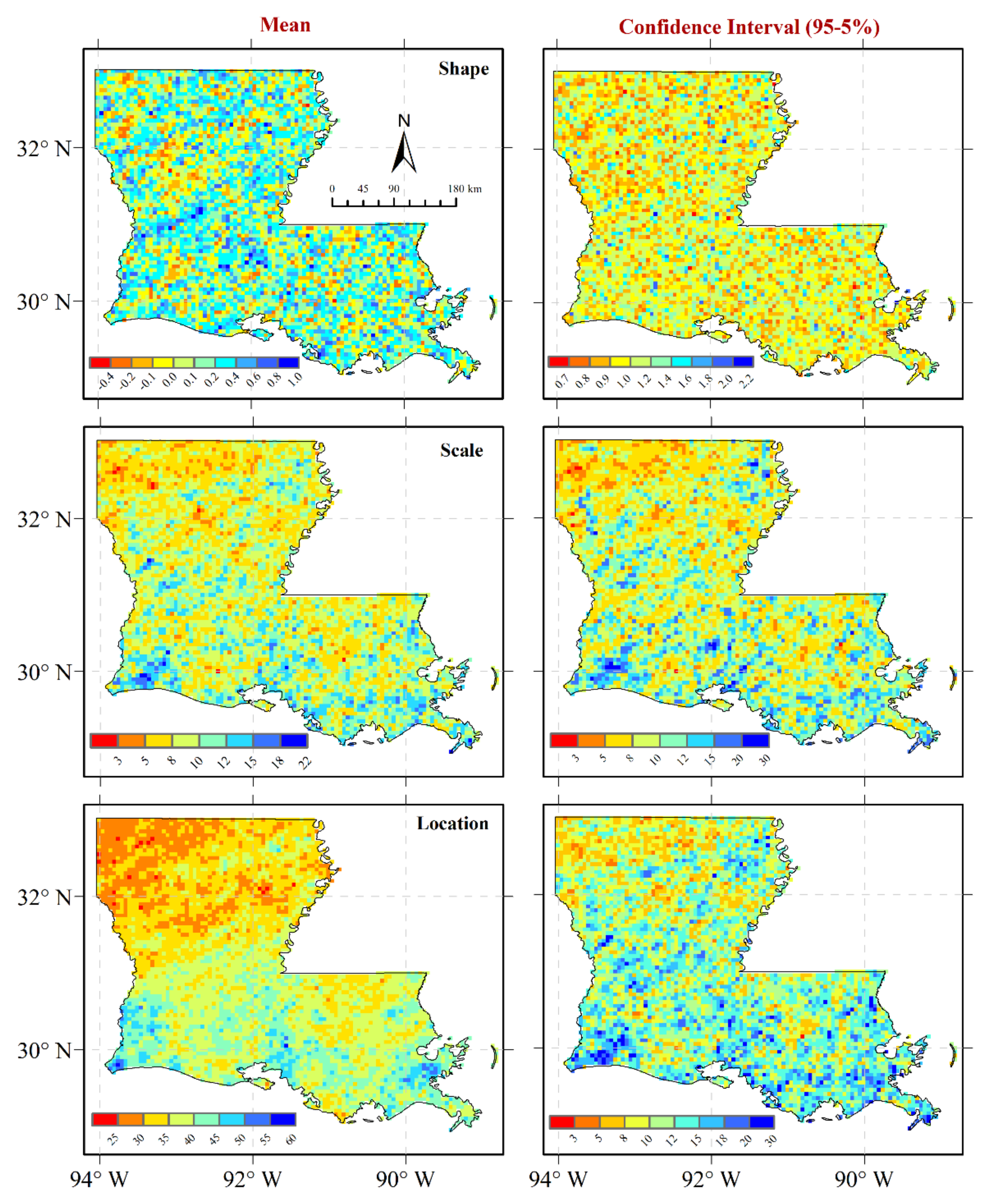
  • The use of the spatial bootstrap regional method resulted in PFE quantiles and distribution parameter spatial fields that are smoother and less noisy compared to the pixel-based approach. Spatial gradients in the PFE quantiles are distinctly evident across the domain of the entire state.
  • Augmenting the sample size and/or the region of influence in the spatial bootstrap showed a significant reduction in the estimated uncertainty of the PFEs at different return periods.
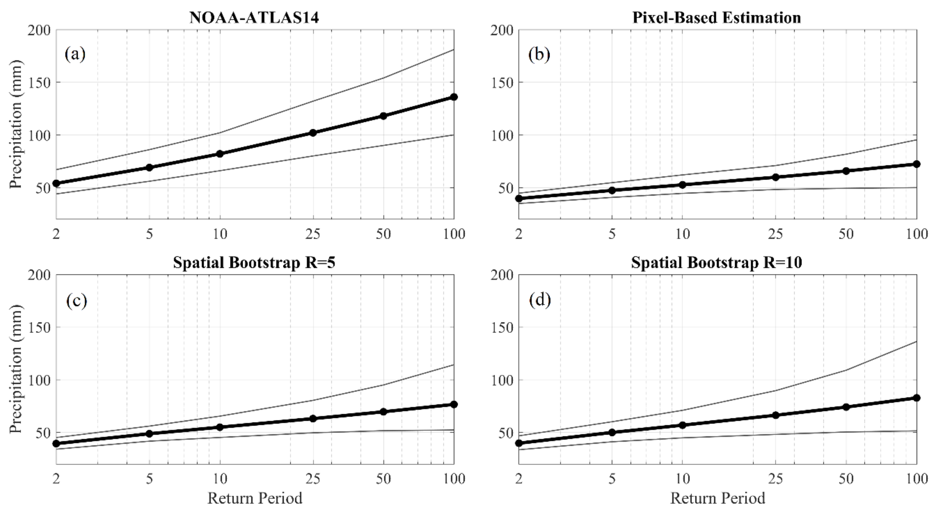
  • Compared to a pixel-based approach, the spatial bootstrap technique is less sensitive to observational and sampling variability and can provide more realistic representation of the PFE confidence intervals. Thus, when compared with the gauge-based NOAA Atlas 14 frequency estimates, PFEs from spatial bootstrap method can be considered more reliable than pixel-based estimation. However, for some cases where QPE estimates have inherent systematic bias especially for extreme rainfall, both of the spatial bootstrap and pixel-based estimation methods resulted in considerable underestimation in PFEs.
The overall results of the current study indicate the potential power of regional spatial bootstrap technique in deriving PFEs from radar-based QPE at high spatial and temporal resolutions. Given the global coverage of satellite data at high spatiotemporal resolution, it is of interest, particularly in regions with scarce in-situ data, to advocate the use of satellite-based PFEs in the design, operation, and planning of infrastructure. Therefore, a robust regional approach, as the spatial bootstrap method, can be very useful in reducing uncertainties associated with satellite-based PFEs. Future studies can also explore a viable approach that combines information from both radar and rain gauge sources to capitalize on their respective strengths and improve the PFE estimation process. Such accurate and regionally representative PFE information are critically needed for various water resources engineering planning and hydrologic design applications.

Author Contributions

H.E. conceived and designed the study, carried out data analysis and drafted the manuscript. E.H. participated in the design of the study, contributed to the interpretation of data and critically revised the draft of the manuscript providing substantial contributions to improve the presentation of results. Both authors read and approved the final manuscript. All authors have read and agreed to the published version of the manuscript.

Funding

This research received no external funding and was supported by internal institutional resources.

Acknowledgments

The authors acknowledge internal institutional funding for supporting the study through the Department of Civil Engineering and the Watershed Flood Center at the University of Louisiana at Lafayette.

Conflicts of Interest

The authors declare no conflict of interest.

References

  1. Seo, D.-J.; Seed, A.; Delrieu, G. Radar and multisensor rainfall estimation for hydrologic applications. In Rainfall: State of the Science; Gebremichael, M., Ed.; American Geophysical Union: Washington, DC, USA, 2010. [Google Scholar]
  2. Pecho, J.; Fasko, P.; Lapin, M.; Gaál, L. Analysis of Rainfall Intensity-Duration Frequency Relationships in Slovakia (Estimation of Extreme Rainfall Return Periods); EGU General Assembly: Vienna, Austria, 2009. [Google Scholar]
  3. Chow, V.T.; Maidment, D.R.; Mays, L.W. Applied Hydrology. In Water Resources Handbook; McGraw-Hill: New York, NY, USA, 1988. [Google Scholar]
  4. Durrans, S.R.; Julian, L.T.; Yekta, M. Estimation of depth-area relationships using radar-rainfall data. J. Hydrol. Eng. 2002, 7, 356–367. [Google Scholar] [CrossRef] [Green Version]
  5. Allen, R.J.; DeGaetano, A.T. Considerations for the use of radar-derived precipitation estimates in determining return intervals for extreme areal precipitation amounts. J. Hydrol. 2005, 315, 203–219. [Google Scholar] [CrossRef]
  6. Olivera, F.; Choi, J.; Kim, D.; Li, M.-H. Estimation of average rainfall areal reduction factors in Texas using NEXRAD data. J. Hydrol. Eng. 2008, 13, 438–448. [Google Scholar] [CrossRef] [Green Version]
  7. Overeem, A.; Buishand, T.A.; Holleman, I. Extreme rainfall analysis and estimation of depth-duration-frequency curves using weather radar. Water Resour. Res. 2009, 45. [Google Scholar] [CrossRef]
  8. Overeem, A.; Buishand, T.A.; Holleman, I.; Uijlenhoet, R. Extreme value modeling of areal rainfall from weather radar. Water Resour. Res. 2010, 46. [Google Scholar] [CrossRef]
  9. Cunnane, C. Methods and merits of regional flood frequency analysis. J. Hydrol. 1988, 100, 269–290. [Google Scholar] [CrossRef]
  10. Burn, D.H. Evaluation of regional flood frequency analysis with a region of influence approach. Water Resour. Res. 1990, 26, 2257–2265. [Google Scholar] [CrossRef]
  11. Burn, D.H. An appraisal of the “region of influence” approach to flood frequency analysis. Hydrol. Sci. J. 1990, 35, 149–165. [Google Scholar] [CrossRef] [Green Version]
  12. Pilona, P.J.; Adamowskib, K.; Alilab, Y. Regional analysis of annual maxima precipitation using L-moments. Atmos. Res. 1991, 27, 81–92. [Google Scholar] [CrossRef]
  13. Svensson, C.; Jones, D.A. Review of rainfall frequency estimation methods. J. Flood Risk Manag. 2010, 3, 296–313. [Google Scholar] [CrossRef] [Green Version]
  14. Hailegeorgis, T.T.; Thorolfsson, S.T.; Alfredsen, K. Regional frequency analysis of extreme precipitation with consideration of uncertainties to update IDF curves for the city of Trondheim. J. Hydrol. 2013, 498, 305–318. [Google Scholar] [CrossRef] [Green Version]
  15. Naghavi, B.; Yu, F.X. Regional frequency analysis of extreme precipitation in Louisiana. J. Hydraul. Eng. 1995, 121, 819–827. [Google Scholar] [CrossRef]
  16. Eldardiry, H.; Habib, E.; Zhang, Y. On the use of radar-based quantitative precipitation estimates for precipitation frequency analysis. J. Hydrol. 2015, 531, 441–453. [Google Scholar] [CrossRef]
  17. Uboldi, F. A spatial bootstrap technique for parameter estimation of rainfall annual maxima distribution. Hydrol. Earth Syst. Sci. 2014, 18, 981–995. [Google Scholar] [CrossRef] [Green Version]
  18. Perica, S. Precipitation Frequency Atlas of the United States, NOAA Atlas 14; USA Department of Commerce, National Oceanic and Atmospheric Adminstration, National Weather Service: Silver Spring, MD, USA, 2013; Volume 9.
  19. Smith, J.A.; Seo, D.J.; Baeck, M.L. An intercomparison study of NEXRAD precipitation estimates. Water Resour. Res. 1996, 32, 2035–2045. [Google Scholar] [CrossRef]
  20. Ciach, G.J.; Krajewski, W.F.; Villarini, G. Product-error-driven uncertainty model for probabilistic quantitative precipitation estimation with NEXRAD data. J. Hydrometeorol. 2007, 8, 1325–1347. [Google Scholar] [CrossRef]
  21. Villarini, G.; Krajewski, W.F.; Ciach, G.J.; Zimmerman, D.L. Product-error-driven generator of probable rainfall conditioned on WSR-88D precipitation estimates. Water Resour. Res. 2009, 45, W01404. [Google Scholar] [CrossRef] [Green Version]
  22. Habib, E. Independent assessment of incremental complexity in NWS multisensor precipitation estimator algorithms. J. Hydrol. Eng. 2013, 18, 143–155. [Google Scholar] [CrossRef]
  23. Seo, D.J. Real-time estimation of rainfall fields using radar rainfall and rain gauge data. J. Hydrol. 1998, 208, 37–52. [Google Scholar] [CrossRef]
  24. Kitzmiller, D.; Miller, D.; Fulton, R.; Ding, F. Radar and multisensor precipitation estimation techniques in National Weather Service hydrologic operations. J. Hydrol. Eng. 2013, 18, 133–142. [Google Scholar] [CrossRef]
  25. Eldardiry, H.; Habib, E.; Zhang, Y.; Graschel, J. Artifacts in Stage IV NWS real-time multisensor precipitation estimates and impacts on identification of maximum series. J. Hydrol. Eng. 2015, 22, E4015003. [Google Scholar] [CrossRef]
  26. Greene, D.R.; Hudlow, M.D. Hydrometeorologic grid mapping procedures. In Proceedings of the AWRA International Symposium on Hydrometeorology, Denver, CO, USA, 13–17 June 1982. [Google Scholar]
  27. Faiers, G.E.; Keim, B.D.; Hirschboeck, K.K. A Synoptic evaluation of frequencies and intensities of extreme three-and 24-hour rainfall in Louisiana. Prof. Geogr. 1994, 46, 156–163. [Google Scholar] [CrossRef]
  28. Madsen, H.; Rasmussen, P.F.; Rosbjerg, D. Comparison of annual maximum series and partial duration series methods for modeling extreme hydrologic events: 1. At-site modeling. Water Resour. Res. 1997, 33, 747–757. [Google Scholar] [CrossRef]
  29. Hosking, J. L-moments: Analysis and estimation of distributions using linear combinations of order statistics. J. R. Stat. Soc. 1990, 52, 105–124. [Google Scholar] [CrossRef]
  30. Martins, E.S.; Stedinger, J.R. Generalized maximum-likelihood generalized extreme-value quantile estimators for hydrologic data. Water Resour. Res. 2000, 36, 737–744. [Google Scholar] [CrossRef]
  31. Hershfield, D.M. Rainfall Frequency Atlas of the United States for Durations from 30 Minutes to 24 Hours and Return Periods from 1 to 100 Years; Technical Paper 40; USA Weather Bureau: Washington, DC, USA, 1961.
  32. Efron, B. Bootstrap methods: Another look at the Jackknife. Ann. Stat. 1979, 7, 1–26. [Google Scholar] [CrossRef]
  33. Hosking, J.R.M.; Wallis, J.R. Regional Frequency Analysis; Cambridge University Press: Cambridge, UK, 1997. [Google Scholar]
  34. Kachroo, R.K.; Mkhandi, S.H.; Parida, B.P. Flood frequency analysis of southern Africa: I. Delineation of homogeneous regions. Hydrol. Sci. J. 2000, 45, 437–447. [Google Scholar] [CrossRef]
  35. Maddox, R.A.; Chappell, C.F.; Hoxit, L.R. Synoptic and meso-α scale aspects of flash flood events 1. Bull. Am. Meteorol. Soc. 1979, 60, 115–123. [Google Scholar] [CrossRef] [Green Version]
  36. Habib, E. Ground based direct measurement. In Rainfall: State of the Science; Testik, F.Y., Mekonnen, G., Eds.; American Geophysical Union: Washington, DC, USA, 2010; Volume 191, pp. 61–77. [Google Scholar]
  37. Weather Bureau. Rainfall Intensity-Frequency Regime—Part 2: The Southeastern United States; Technical Paper No. 29 (TP-29); USA Weather Bureau: Washington, DC, USA, 1958.
  38. Vogel, R.M.; Shallcross, A.L. The moving blocks bootstrap versus parametric time series models. Water Resour. Res. 1996, 32, 1875–1882. [Google Scholar] [CrossRef]
  39. Ciach, G.J.; Morrissey, M.L.; Krajewski, W.F. Conditional bias in radar rainfall estimation. J. Appl. Meteorol. 2000, 39, 1941–1946. [Google Scholar] [CrossRef]
  40. Habib, E.; Qin, L. Application of a radar-rainfall uncertainty model to the NWS multi-sensor precipitation estimator products. Meteorol. Appl. 2013, 20, 276–286. [Google Scholar] [CrossRef]
  41. Wazneh, H.; Chebana, F.; Ouarda, T.B. Delineation of homogeneous regions for regional frequency analysis using statistical depth function. J. Hydrol. 2015, 521, 232–244. [Google Scholar] [CrossRef]
Figure 1. (a) Spatial distribution of the hourly Mean Annual Maxima (MAM; in mm). (b) The average month of AMS occurrence in each pixel. (c) The average 6-h of AMS occurrence in each pixel. Results are based on the period of study (2002–2012).
Remotesensing 12 03767 g001
Figure 2. The GEV distribution parameters (shape, scale, and location parameters) from the pixel-based approach. Left Panels: Mean of 500 bootstrap runs. Right Panels: The confidence width (95–5% percentiles).
Remotesensing 12 03767 g002
Figure 3. The GEV distribution parameters (shape, scale, and location parameters) from the spatial bootstrap (region-based) approach. Left Panels: Mean of 500 bootstrap runs. Right Panels: the confidence width (95–5% percentiles).
Remotesensing 12 03767 g003
Figure 4. The rainfall depth (in mm) and the confidence width (95–5% percentiles) corresponding to 2-year return period from the pixel-based (upper panels) and spatial bootstrap approaches (region-based) (lower panels).
Remotesensing 12 03767 g004
Figure 5. The rainfall depth (in mm) and the confidence width (95–5% percentiles) corresponding to 10-year return period from the pixel-based (upper panels) and spatial bootstrap approaches (region-based) (lower panels).
Remotesensing 12 03767 g005
Figure 6. (a) the mean annual maxima rainfall depth extracted from NOAA Atlas 14 gauges and the corresponding radar-pixel (each color represents one of the 33 gauges in Louisiana retrieved from NOAA HDSC web-based data server). (b) same as (a) but reporting the coefficient of variation. (c) comparison of AMS from gauge data and radar-based estimates (for common period 2002–2010) at the location of two example NOAA Atlas-14 gauges (indicated in Figure 1a).
Remotesensing 12 03767 g006
Figure 7. The range of AMS from gauge data, radar pixel, and radar-based regional sample considering a radius of 5 and 10 pixels. Each bar ranges between the minimum and maximum value in AMS sample extracted at the location of gauge (see Figure 1a for gauges locations).
Remotesensing 12 03767 g007
Figure 8. Precipitation Frequency Estimates (PFE) and (95–5%) confidence limits using different estimation approaches at the location of Gauge (1).
Remotesensing 12 03767 g008
Figure 9. Precipitation Frequency Estimates (PFE) and (95–5%) confidence limits at the location of Gauge (2) based on (a) NOAA-Atlas14, (b) pixel-based approach, and (c,d) regional spatial bootstrap with a region of R = 5 pixels (c) and R = 10 pixels (d).
Remotesensing 12 03767 g009
Figure 10. Percentage change in mean quantiles and confidence interval (95–5%) when using the spatial bootstrap method with sample size of 11 and 30, compared to NOAA Atlas 14 gauge-based PFES (only 10 and 25-year return periods are shown).
Remotesensing 12 03767 g010
Table 1. The NOAA Atlas 14 gauges selected in our study to evaluate the spatial bootstrap approach when using radar-based precipitation estimates.
GaugeLatitudeLongitudeNOAA Atlas14
AMS Size
Gauge (1)30.12°−93.23°49 years
Gauge (2)29.23°−90.00°26 years
Gauge (3)29.99°−90.25°64 years
Publisher’s Note: MDPI stays neutral with regard to jurisdictional claims in published maps and institutional affiliations.

