Article

A Model-Based Volume Estimator that Accounts for Both Land Cover Misclassification and Model Prediction Uncertainty

by
Jessica Esteban
1,2,*,
Ronald E. McRoberts
3,
Alfredo Fernández-Landa
2,
José Luis Tomé
2 and
Miguel Marchamalo
1
1
Departamento de Ingeniería y Morfología del Terreno, Laboratorio de Topografía y Geomática, Universidad Politécnica de Madrid, 28040 Madrid, Spain
2
AGRESTA Sociedad Cooperativa, 28012 Madrid, Spain
3
Department of Forest Resources, University of Minnesota, St. Paul, MN 55108, USA
*
Author to whom correspondence should be addressed.
Remote Sens. 2020, 12(20), 3360; https://doi.org/10.3390/rs12203360
Submission received: 12 August 2020 / Revised: 25 September 2020 / Accepted: 10 October 2020 / Published: 15 October 2020
(This article belongs to the Special Issue Advances in Remote Sensing for Global Forest Monitoring)

Abstract

:
Forest/non-forest and forest species maps are often used by forest inventory programs in the forest estimation process. For example, some inventory programs establish field plots only on lands corresponding to the forest portion of a forest/non-forest map and use species-specific area estimates obtained from those maps to support the estimation of species-specific volume (V) totals. Despite the general use of these maps, the effects of their uncertainties are commonly ignored with the result that estimates might be unreliable. The goal of this study is to estimate the effects of the uncertainty of forest species maps used in the sampling and estimation processes. Random forest (RF) per-pixel predictions were used with model-based inference to estimate V per unit area for the six main forest species of La Rioja, Spain. RF models for predicting V were constructed using field plot information from the Spanish National Forest Inventory and airborne laser scanning data. To limit the prediction of V to pixels classified as one of the main forest species assessed, a forest species map was constructed using Landsat and auxiliary information. Bootstrapping techniques were implemented to estimate the total uncertainty of the V estimates and accommodated both the effects of uncertainty in the Landsat forest species map and the effects of plot-to-plot sampling variability on training data used to construct the RF V models. Standard errors of species-specific total V estimates increased from 2–9% to 3–22% when the effects of map uncertainty were incorporated into the uncertainty assessment. The workflow achieved satisfactory results and revealed that the effects of map uncertainty are not negligible, especially for open-grown and less frequently occurring forest species for which greater variability was evident in the mapping and estimation process. The effects of forest map uncertainty are greater for species-specific area estimation than for the selection of field plots used to calibrate the RF model. Additional research to generalize the conclusions beyond Mediterranean to other forest environments is recommended.

Graphical Abstract

1. Introduction

Forest and other wooded land environments provide numerous ecosystem services that contribute directly or indirectly to improving our well-being. They play an important role in mitigating climate change through carbon sequestration, combating desertification, maintaining biodiversity, protecting soil and water resources, and supplying wood and other forest products [1] (pp. 285–299). In light of the significance of these roles, accurate and updated information suitable for assessing forest resources is needed. National forest inventories (NFIs) were originally motivated by a need for information on forest area, volume, and increment of growing stock and the amount of timber [2]. Since then, many countries have established their NFI programs as the primary sources of forest information necessary for forest management and policy formulation [3,4].
NFI data include measurements of individual trees on plots selected using probabilistic sampling designs. Tree measurements include height and diameter, which are then used to predict individual tree attributes such as volume and biomass [5]. To increase the efficiency of inventory sampling designs, maps can be used in the design phase to select the locations of the field plots [6] and in the estimation phase to increase precision [7,8]. Of the 37 countries for which Tomppo et al. [9] include NFI reports, six countries use a forest/non-forest map to determine where to establish their field plots. Among them is Spain, where permanent sampling plots are established systematically at the intersections of a 1-km × 1-km grid in the portion of the Spanish National Forest Map (SNFM) classified as forest land. Therefore, the SNFM is the base mapping layer for the Spanish National Forest Inventory (SNFI), both of which are updated on a 10-year cycle [10]. The most recent versions of the SNFM are based on the photointerpretation of aerial photography and digitization of polygons that are classified with respect to the vegetation present in the area [11].
Traditional forest inventories have the disadvantage of being expensive, especially in areas with poor road infrastructure [12]. In the last decades, remote sensing (RS) technologies have emerged as an auxiliary data source that alleviates some of this limitation by increasing the precision of inventory estimates and reducing the cost of forest resources assessment [13]. These technologies typically entail constructing a model that represents the relationship between the RS data and field plot data. The model is applied to predict forest attributes where field plots are lacking, thereby producing spatially continuous forest attribute information [14]. These modeling applications have led to inferential approaches guided by the properties of the ground data [15]. In particular, model-based (MB) inferential approaches can be used when models are constructed using data collected from non-probability training samples and data external to the area of interest [16]. This feature makes MB inference an interesting option for areas where design-based inference is limited due to remoteness and inaccessibility [17]. However, the effectiveness of this approach relies on the correctness of the model, and consequently, population parameter estimators may be biased and imprecise if the model is incorrect [18,19]. Hence, the estimation of forest population parameters and a rigorous assessment of their uncertainties are necessary to produce reliable estimates.
In this context, reliable methods for propagating the main sources of uncertainty associated with forest predictions have been developed [12,20,21]. As noted previously, forest maps can be used as masks in the design phase to restrict the establishment of field plots and in the estimation phase to restrict the application of the models. Most current reports in the literature assume that these maps are without error [17,18], but very few have analyzed the effects of this source of uncertainty on the uncertainty of forest attribute estimates. Rodríguez-Veiga et al. [22] used multiple forest masks constructed using MODIS and ALOS PALSAR data to estimate total aboveground biomass for Mexico. Their study demonstrated that different forest masks had large impacts on the estimation of national carbon stocks due to the discrepancies in the forest extent estimated from each forest mask. Li et al. [23] found substantial differences in the regional climate modeling outputs when the uncertainty of the MODIS land cover products used was considered.
These studies showed how the uncertainty inherent in forest maps affects the reliability of estimates. Both national estimates and uncertainties of the estimates are required for NFI reporting and are specifically required for greenhouse gas inventories. In particular, the Intergovernmental Panel on Climate Change (IPCC) states as a guideline that uncertainties should be reduced as far as practicable [24]. However, the satisfaction of this guideline implies that before uncertainties can be reduced, they must first be properly estimated. Failure to estimate the uncertainty associated with forest maps used to restrict the establishment of ground plots and application of models could lead to imprecise estimates and under-estimated uncertainties, thereby leading to reporting estimates that would fail to comply with the IPCC guidelines. In addition, sampling completely within a forest mask facilitates the estimation of deforestation but not reforestation or afforestation outside the map unless the mask is updated frequently. In the last decades, Spain has reported an expansion of forest area because of the naturalization of marginal agricultural land due to rural abandonment and of afforestation policies through the Common Agricultural Policy [25].
The goal of this study is to estimate the effects of the uncertainty of forest species maps used in the sampling and estimation processes. To this end, we addressed the following objectives: (1) to provide pixel-level volume (V) predictions for a large region using three sources of information: SNFI ground plot data, multispectral data, and airborne laser scanning (ALS) data; (2) to estimate the total MB uncertainty of the large area V estimates taking into account both the uncertainty of a forest species map that guided the selection of plot locations and application of models, and sampling variability; and (3) to estimate the relative contributions to the total uncertainty in the large area estimates of each of the components. MB inference used random forests V models specific to each of the main forest species of La Rioja whose spatial distributions were initially determined from a forest species map constructed using Landsat imagery. Random forests (RF) predictive V models and RF classification models were constructed.

2. Materials and Methods
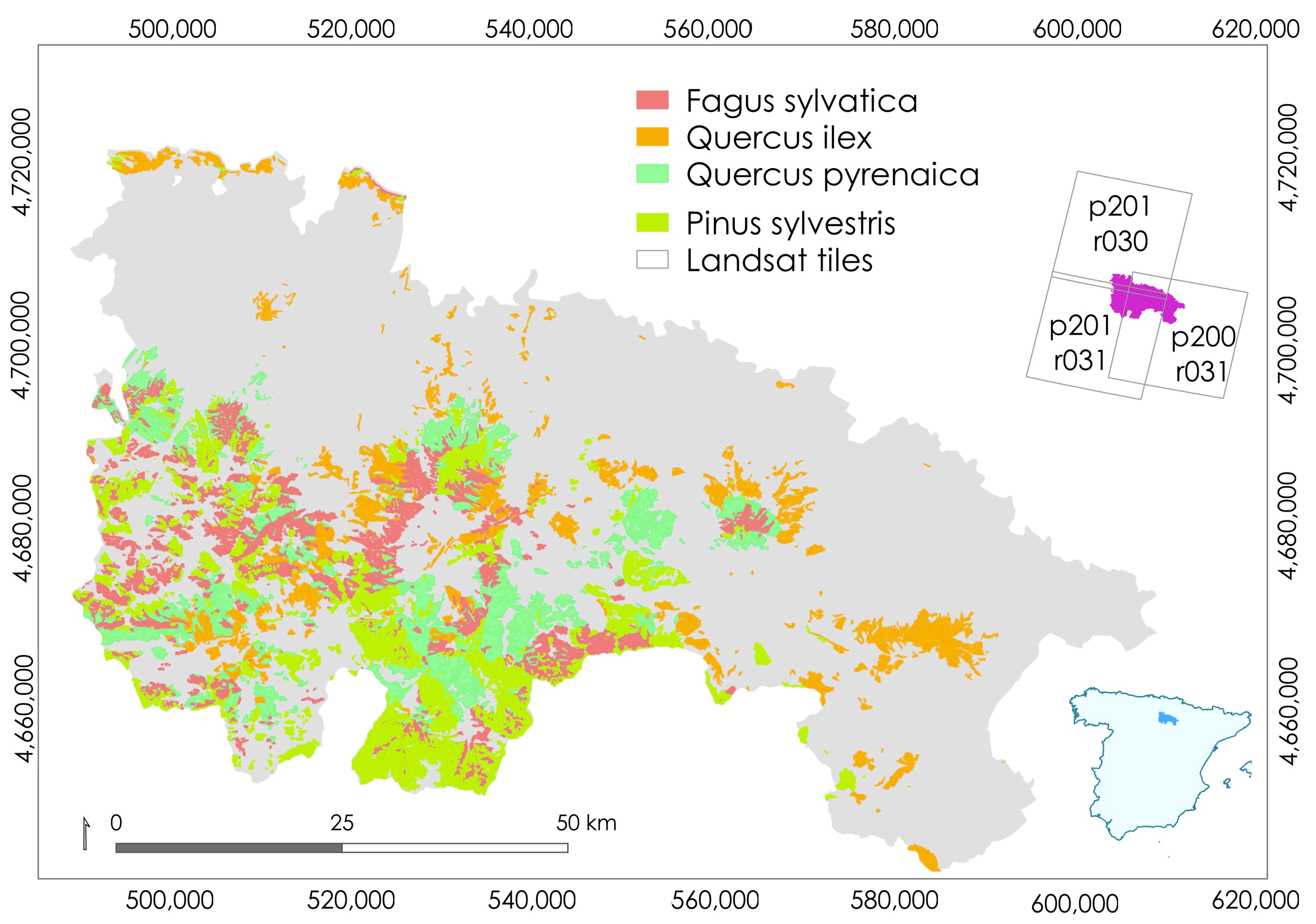
2.1. Study Area

The study area was La Rioja, Spain, covering an area of 5045 km2 (Figure 1). This province in the north of Spain borders mostly Navarre, Castile, and Leon, and also the Basque Country and Aragon. La Rioja is surrounded by two large relief units with elevations ranging from 260 to approximately 2300 m. This large altitudinal gradient contributes to rich vegetative diversity ranging from coniferous forests, deciduous forests, mixed forests, and shrub lands to grasslands in a relatively small area. According to the SNFI, forest land (without considering shrublands and grasslands) covers 34.7% of La Rioja with the main forest species, in order of area: Pyrenean oak (Quercus pyrenaica Willd), Scots pine (Pinus sylvestris L.), beech (Fagus sylvatica L.), and holly oak (Quercus ilex L.) [26] (p. 11). The remaining part of the study area is lowlands composed of unirrigated and irrigated fields where the landscape becomes more homogenous. La Rioja includes important natural environmental aspects such as Sierra de Cebollera Natural Park and Urbion Lake, among others. In addition, 24% of La Rioja was declared a Biosphere Reserve by UNESCO.

2.2. Data

Three types of data were used in this research: the SNFI field data, multispectral data, and ALS data.

2.2.1. Spanish National Forest Inventory (SNFI)

The 4th SNFI in La Rioja was conducted between 2011 and 2012 using permanent sample plots established systematically at the intersections of a 1 km × 1 km grid in areas identified as forest land by the SNFM (E: 1:25,000) (SNFM25) [10]. The methodology for producing SNFM25 includes three phases: (i) the manual digitalization of polygons with homogenous forest structure and forest species on screen by photo-interpretation, (ii) field monitoring, and (iii) quality control. Field visits are programmed for quality control over the polygons whose digitalization are problematic [10]. Discrepancies between SFM25 and SNFI are analyzed, and modifications are made if needed.
The SNFI sample units consist of four circular concentric plots of radius 5, 10, 15, and 25 m. Trees with diameter at breast height (DBH) of at least 75 mm are measured in a 5 m radius plot; trees with DBH > 125 mm are measured in a 10 m radius plot; trees with DBH > 225 mm are measured in a 15 m radius plot; and only trees with a DBH > 425 mm are measured in the 25 m radius plot [10,27]. For each tree, DBH, total height, forest species, and the tree’s position relative to the plot center (direction and distance) are recorded. Species-specific allometric models were used with measured DBH and height to predict individual tree volumes which were weighted to predict the total plot volume. The main difficulty in combining SNFI plot data with ALS measurements is discrepancies between the attribute measured in field and the ALS data assigned due to center plot coordinate errors [28]. Therefore, only plots for which the maximum height of a measured tree, hmax, was within ±4 m of the 99th ALS height percentile were considered. The deletion of 153 of these plots altered the systematic nature of the grid-based sample with the result that the remaining sample consisting of 1095 SNFI plots was considered a purposive sample, albeit with systematic components. This sample was used to construct the volume models (Section 2.4.3).

2.2.2. Multispectral and Auxiliary Data

The study area is covered by three Landsat scenes with paths (p) and rows (r): p201 r031, p200 r031, and p200 r030 (Figure 1). For each scene, predominantly cloud-free Landsat 5 Thematic Mapper (TM) images from 1 June to 31 August for 2010 were used to construct an updated forest species map (Section 2.4.2). The reason behind the decision to use Landsat 5 data is their availability for free and absence of sensor malfunction problems as occurred in Landsat 7. Annual summer composites based on the greenest pixels available defined by Normalized Difference Vegetation Index (NDVI) were constructed using the Google Earth Engine Python and Javascript Application Programming Interfaces [29] and resampled to the corresponding 25 m × 25 m ALS cell size (Section 2.2.3). For this study, we used the following bands: blue (0.45–0.52 µm), green (0.52–0.60 µm), red (0.63–0.69 µm), near infrared (NIR; 0.76–0.90 µm), and two shortwave IR bands (SWIR1, 1.55–1.75 µm; and SWIR2, 2.08–2.35 µm). Three vegetation indexes were derived from the annual summer composites: NDVI, the Normalized Difference Moisture Index (NDMI) and the Normalized Burn Ratio (NBR). Finally, elevation information was derived from a 25 m × 25 m digital elevation model downloaded from the Spanish National Center of Geographic Information.

2.2.3. Airborne Laser Scanning (ALS) Data

ALS data were acquired between August and October 2010, during leaf-on conditions by the Spanish National Programme of Aerial Orthophotography with a mean pulse density of 0.5 points per m2 and vertical root mean square error (RMSE) ≤ 0.20 m. ALS tiles were processed using FUSION software [30] to construct a 2-m digital elevation model from the ground points, thereby facilitating the estimation of height above the ground surface for each ALS vegetation point. Following the removal of ground points with heights less than 2 m, 15 forest structure metrics were calculated for both the SNFI plots and for the 25 m × 25 m cells that tessellated the study area and served as population units. ALS metrics included mean, variance (varia), standard deviation (stdev), coefficient of variation (cv), interquartile range (iq), kurtosis (kurto), percentiles (ranging from the 1st to 99th percentile: p1, p5, p25, p50, p75, p95, and p99), canopy relief ratio (crr), and forest canopy cover (lfcc).
The methodological framework is illustrated in Figure 2.

2.3. Statistical Techniques

2.3.1. Overview

Three primary statistical techniques were used in the study. First, the RF method (Section 2.3.2) was used for classification to construct a forest species map (Section 2.4.2) and to predict volume (V) for individual population units (Section 2.4.3 and Section 2.4.4). Second, the sampling design used to acquire the model calibration data had both systematic and purposive features (Section 2.2.1). As a result of the purposive features, model-based (MB) population parameter estimation methods were used (Section 2.3.3). Third, because the V estimation procedure had multiple estimation and uncertainty components and because analytical procedures for estimating uncertainties associated with the RF approach are generally not available, bootstrapping procedures were used. For the estimation of uncertainties associated with the forest species map, pairs bootstrapping (p) was used (Section 2.3.4). However, for the estimation of uncertainties associated with volume estimation, for which the model calibration data were acquired using a design with substantial systematic components, wild bootstrapping (w) was used (Section 2.3.4). These three statistical techniques are described in greater detail in the sections that follow immediately.

2.3.2. Random Forests (RF)

Forest population parameter estimation using models that represent relationships between inventory variables and RS observations has become relatively common in recent decades [31,32,33]. For this study, RF [34] was selected as the model or prediction technique due to its utility and its popularity [35,36]. Multiple studies support the reliability of RF as a robust classifier and prediction model for forest attributes when used with RS auxiliary data [37,38,39,40,41]. Although the term “regression” has often been used in combination with RF, in this study, the term “prediction model” was used to avoid confusion with linear or nonlinear regression models.
RF consists of a combination of decision tree predictors, each of which is preceded by a bootstrap resample usually consisting of 2/3 of the original sample data. The remaining 1/3 of the original sample is retained as another subset called out-of-bag (oob) and is used for internal error estimation [42]. For this study, RF models were calibrated using the R package RandomForest [43] with the default settings of number of trees (500) and of predictor variables (mtry) tested at each node (mtry = p/3 for prediction or mtry = sqrt (p) for classification, where p is the total number of predictor variables).

2.3.3. Model-Based (MB) Estimation

For the estimation of species-specific V mean, MB inferential methods that do not require probability samples were used. As previously noted (Section 2.2.1), the available SNFI sample was considered a non-probability, purposive sample. In addition, new forest species maps constructed as part of the uncertainty estimation procedure (Section 2.4.2 and Section 2.4.4) may extend into areas originally classified as non-forest in which case no sample plots will be available, thereby further altering the systematic nature of the sample and deviating from a probability sample. The MB estimator of the species-specific V mean is
μ ^ M B = 1 N i = 1 N v ^ i ,
where v ^ i is the RF prediction of v for the ith population unit (pixel, map unit) and N is the total number of population units for each forest species for which V prediction models were applied.

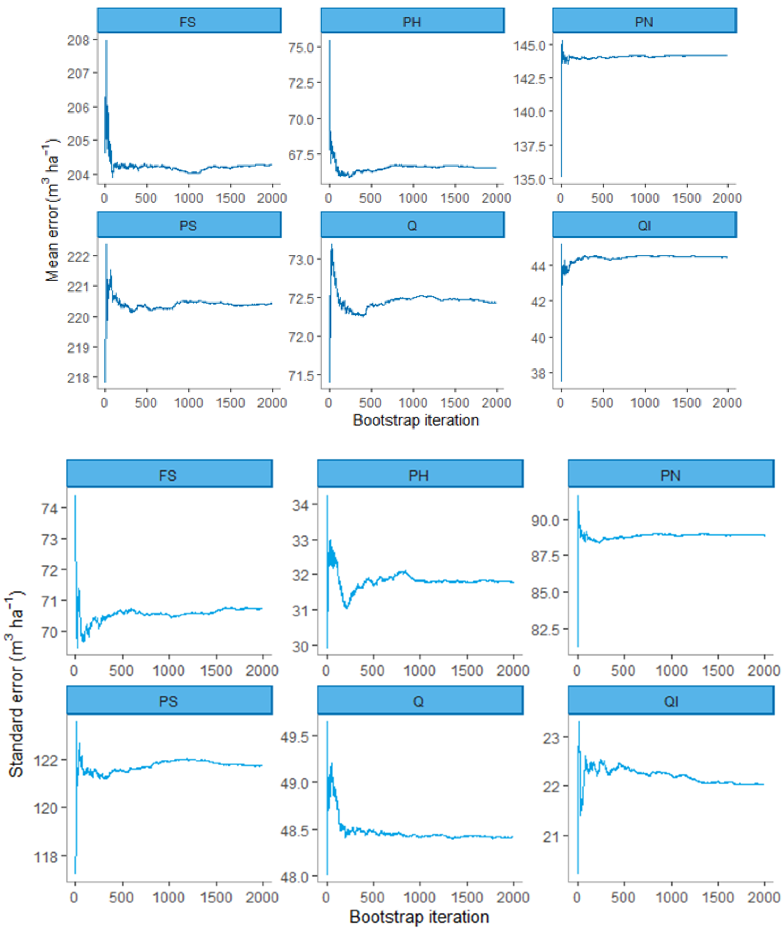
2.3.4. Bootstrapping
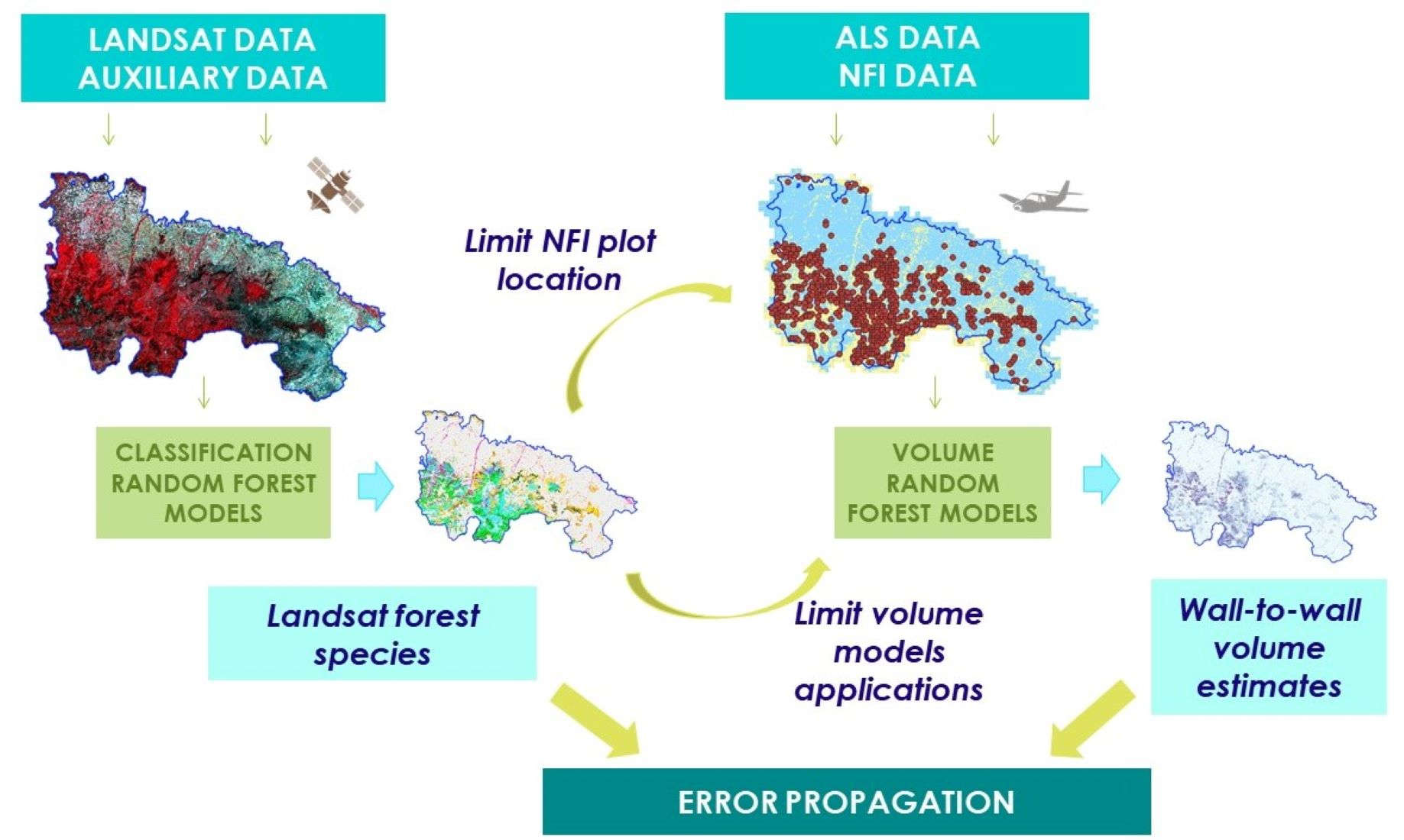
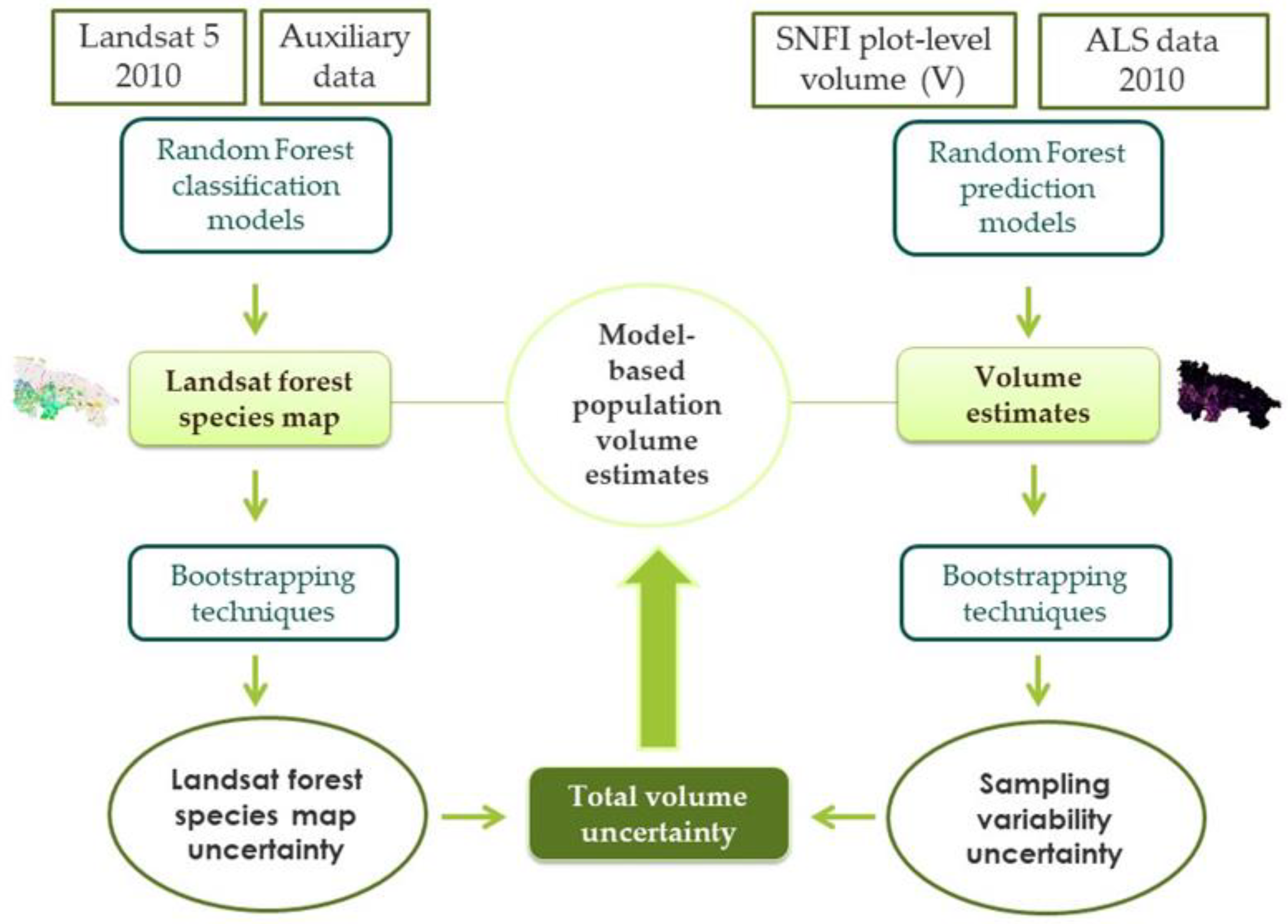
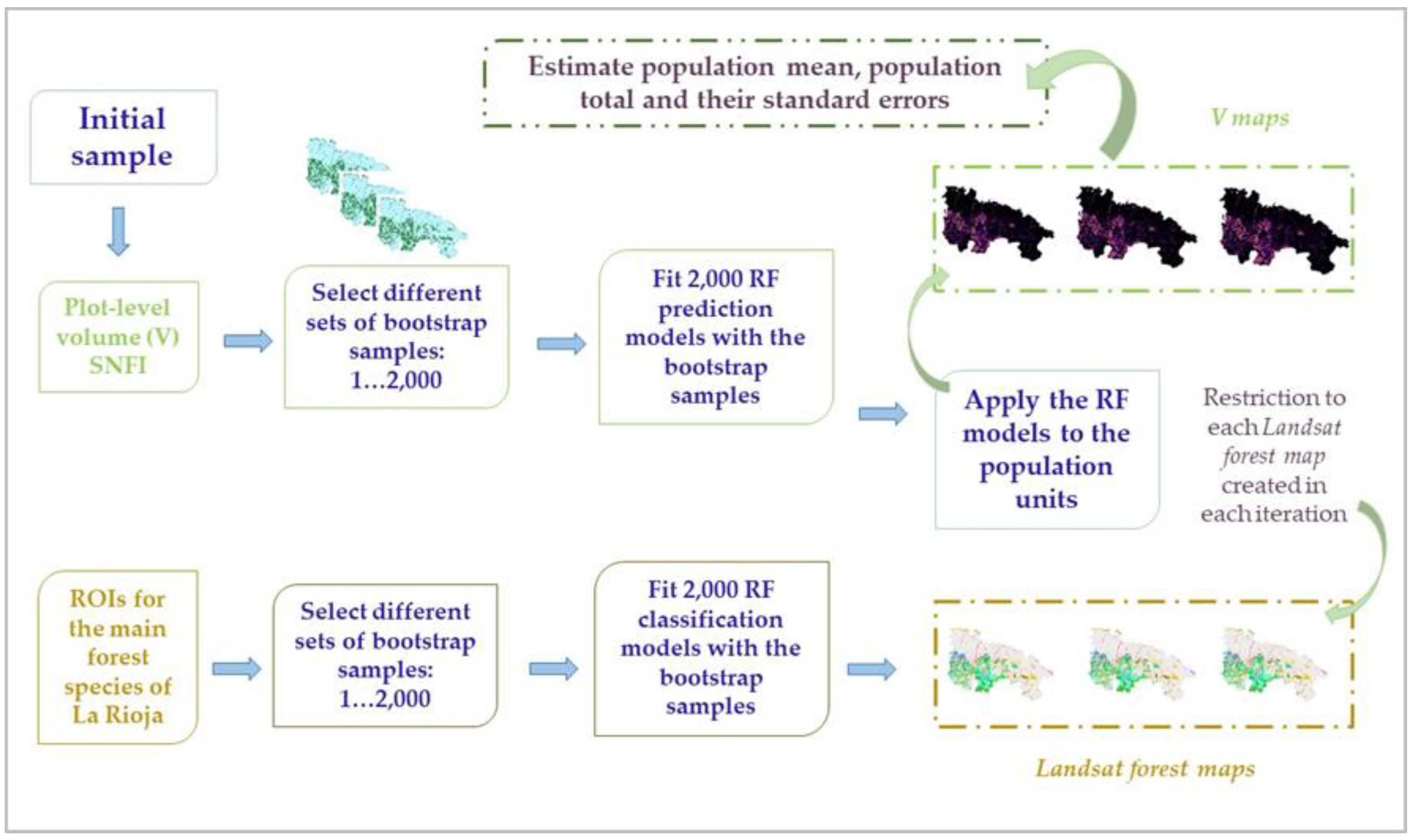
Four primary sources of uncertainty are associated with all MB predictions: (i) model misspecification, (ii) uncertainty in the values of the independent variables, (iii) residual variability around model predictions, and (iv) uncertainty in the model predictions resulting from the effects of sampling variability as they affect the model calibration dataset [16]. For this study, the RF prediction technique was assumed to be sufficiently accurate that model misspecification was not considered problematic (Section 3.1.2). Furthermore, uncertainty in the values of the independent variables were considered negligible. Finally, for large forest areas, the effects of model prediction uncertainty resulting from sampling variability dominate the effects of residual uncertainty [44]. Therefore, for this study, all the sources were ignored except the effects of sampling variability on the V model calibration dataset. When a regression model is used for prediction purposes, the effects of this sampling variability can be expressed in terms of the covariances for the model parameter estimates. However, when non-parametric prediction techniques such as RF are used, more complex techniques merit consideration [44]. For these situations, bootstrapping techniques [33,45,46] have emerged as robust alternatives to analytical variance estimators and uncertainty propagation [47,48].
Two bootstrapping techniques were considered for this study to estimate the uncertainty of the MB population parameter estimates: pairs bootstrapping [49] and wild bootstrapping [50]. Pairs bootstrapping, also characterized as non-parametric bootstrapping [51], entails randomly selecting with replacement a resample of the original data of the same size as the original sample. With pairs bootstrapping, the resample will omit some of the original sample units but include some of the original sample units multiple times. A basic bootstrap principle is that the resampling procedure should mimic the original sampling scheme [50,51,52,53] (p. 2). Thus, unless the original sample was acquired using simple random sampling, conventional RF that uses pairs bootstrapping does not preserve the underlying spatial structure of systematic sample, or samples with substantial systematic components such as the SNFI field plot sample.
As an alternative to pairs bootstrapping, Liu [50] proposed the wild bootstrap, which retains the full set of original sample units and, therefore, retains any original spatial structure in the sample data. Wild bootstrapping entails two steps. First, predictions and residuals for the original sample are calculated using an arbitrary prediction technique. Second, the wild bootstrap resample is constructed as the predictions plus products of the residuals and a randomly selected variable from a distribution with mean 0 and standard deviation of 1 [54,55,56]. For this study, a standard normal distribution was used but with truncation of values less than −2.0 and greater than 2.0. The advantage of wild bootstrapping is that it preserves the original spatial structure of the data, but it requires the calculation of predictions and residuals for the original sample units using another technique for which pairs bootstrapping is a viable candidate and is easily implemented for continuous response variables.

2.4. Analyses

2.4.1. Overview

The analyses focused on estimating species-specific mean and total V. A key feature of the study was that RF models for predicting V were constructed using data for only those field plots that were located in the forest portion of a forest species map. Thus, uncertainty in the estimates of mean and total V must incorporate the uncertainty from two sources: uncertainty in the forest species map and the sampling variability in the model calibration data. The analyses focused on four tasks. First, a forest species map was constructed using training and Landsat data. The map was first used to estimate species-specific areas using MB methods and their standard errors using pairs bootstrapping (Section 2.4.2). Second, the effects of sampling variability associated with the portion of the SNFI field dataset used to calibrate the models were estimated using wild bootstrapping (Section 2.4.3). Third, the map was used to limit the plots whose data were used to construct the RF V models and to limit the population units to which the models were applied. MB methods were used to estimate mean and total V and their standard errors (SE) (Section 2.4.4). Finally, total uncertainty was estimated by combining the effects of uncertainty in the forest species map and sampling variability in the model calibration data (Section 2.4.5). Methods for accomplishing these tasks are described in the sections that follow immediately.

2.4.2. The Forest Species Map and the Effects of Its Uncertainty on Area Estimates

A forest species map, hereafter called the Landsat forest species map, was constructed for the study area (Figure 1) to depict the six dominant forest species of La Rioja: Fagus sylvatica (FS), Pinus halepensis (PH), Pinus nigra (PN), Pinus sylvestris (PS), Quercus pyrenaica/faginea (Q), and Quercus ilex (QI). The remaining forest species occurring in the study area were classified into two general groups designated as “Other coniferous” (OC) and “Other broadleaves” (OB). Non-forest areas such as water bodies, agricultural areas, bare soil, urban fabric, shrublands and grasslands were merged into a single non-forest (NF) class. Training areas were digitalized using the combination of fine resolution imagery and information on forest species from the SNFM25 map which, for purposes of training area delimitation, were considered as “ground truth” and not subject to uncertainty. Once the training areas were delineated, a stratified sample of 100 points was selected for which the nine species classes served as strata. The number of points per training area could be one, several, or no points. Spectral bands, vegetation indexes, and auxiliary information (Section 2.2.2) were used as predictor variables for the calibration of the RF classification models. To assess the accuracy of the Landsat forest species map, the RF oob error was analyzed. This oob error estimation is considered a reliable source that can replace a test dataset independent of the training dataset for the algorithm [42].
Uncertainty in the Landsat forest species map induces uncertainty in the species-specific area estimates. Hence, to estimate the effects of this source of uncertainty, a 4-step bootstrap procedure was used:
(1)
A pairs bootstrap resample was selected from the training data used to calibrate the RF classification model,
(2)
A new Landsat forest species map was constructed by applying a new RF classification model based on the resample from step (1),
(3)
The area for each of the dominant forest species, k, for each bootstrap iteration, b, was estimated as the product of the number of pixels classified as the species and the pixel area and was denoted A ^ p   b k where the subscript “p” indicates that pairs bootstrapping was used,
(4)
Steps (1)–(3) were replicated 2000 times,
(5)
The MB estimates of species-specific areas and their SEs were estimated as,
A ^   p   m a p k = 1 n b o o t b = 1 n b o o t A ^   p   b k
and
S E ( A ^   p   m a p k ) = 1 n b o o t 1   b = 1 n b o o t ( A ^   p   b k A ^   p   m a p k ) 2
where the subscript “map” indicates that only the uncertainty in the Landsat forest species map was incorporated into Equation (3), and the subscript “b” indexes the bootstrap resamples.

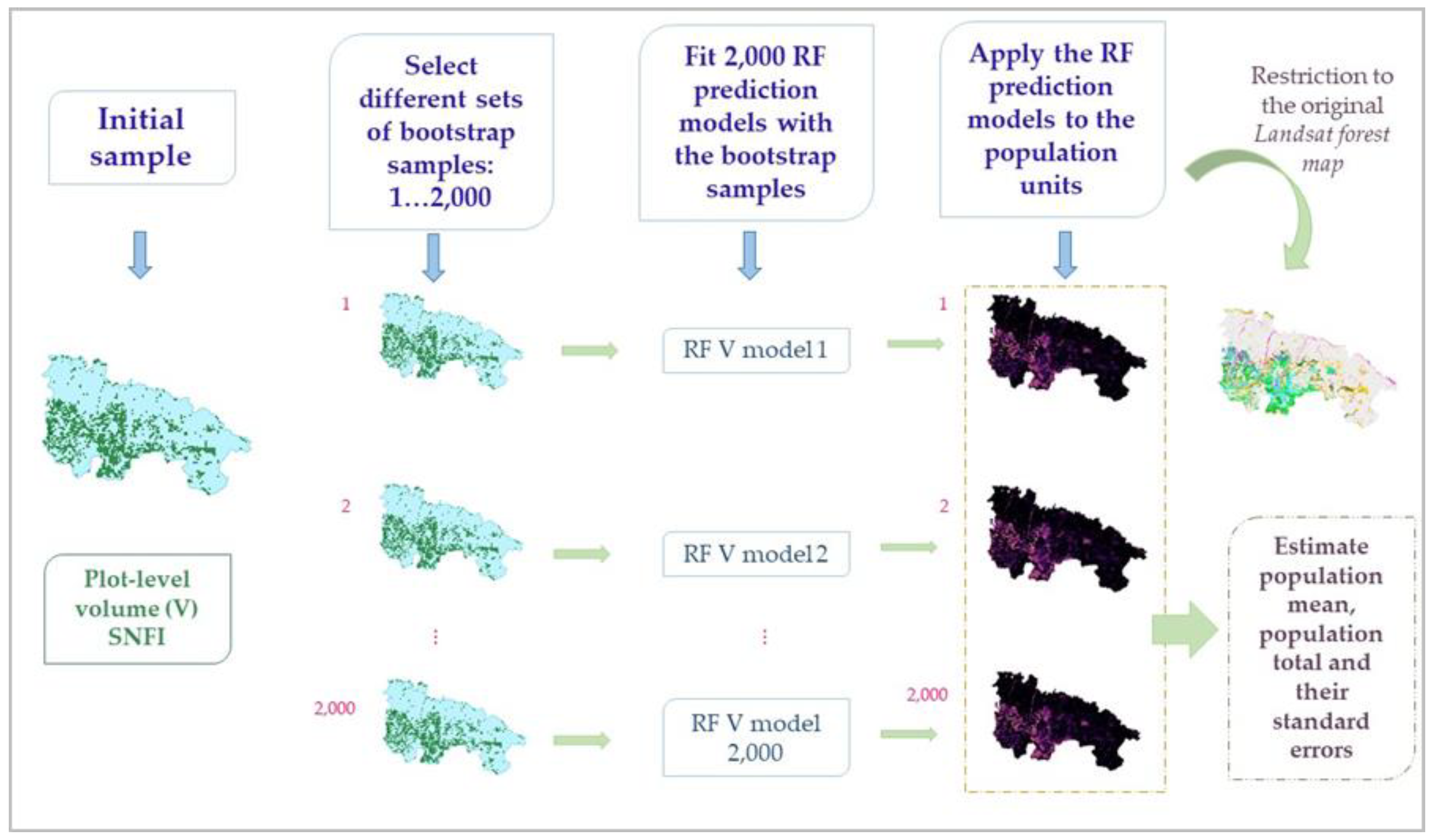
2.4.3. The Effects of Sampling Variability in the Volume Model Calibration Data on Volume Estimates

Species-specific RF models of the relationship between mean V per unit area (m3/ha) as the response variable and the set of ALS metrics as the predictor variables (Section 2.2.3) were constructed for each of the six dominant forest species in La Rioja (FS, PH, PN, PS, Q, QI) (see Table A1 in Appendix A). Although OB and OC were discriminated on the Landsat forest species map, V models for OB and OC were not constructed and, therefore, mean and total V for these forest species were not estimated for this study.
RF models were calibrated using the original SNFI field plot dataset (Table 1) subject to two constraints: (i) only data for plots that were in forest land portion of the original Landsat forest species map, and (ii) only data for plots whose ground measurements were of that forest species without regard to the forest species predicted by the Landsat forest species map.
For each forest species, the species-specific V model was used to predict V for each population unit classified as that species in the original Landsat forest species map. Corresponding SEs for the estimates of mean and total V were estimated using a 7-step wild bootstrapping procedure (Figure 3):
(1)
Select a wild bootstrap resample from the SNFI field plot dataset subject to the two previously noted constraints,
(2)
Calibrate the species-specific RF V models,
(3)
For each species, k, predict V for all population units classified as that species in the original Landsat forest species map,
(4)
Estimate mean species-specific V as V ^   w   b k using Equation (1) and total V, V T   ^ w   b k , as the product of the estimates of mean V and the area, A ^ k , from the original Landsat forest species map,
V T   ^ w   b k = V ^   w   b k · A ^ k
where the subscript “w” indicates that wild bootstrapping was used.
(5)
Repeat steps (1)–(4) 2000 times,
(6)
Estimate species-specific mean V and its SE as,
V ^   w   p l o t k = 1 n b o o t b = 1 n b o o t   V ^   w   b k
with
S E ( V ^   w   p l o t k ) = 1 n b o o t 1   b = 1 n b o o t ( V ^   w   b k V ^   w   p l o t k ) 2 ,
(7)
Estimate species-specific total V and its SE as,
V T   ^ w   p l o t k = 1 n b o o t b = 1 n b o o t   V T   ^ w   b k
with
S E ( V T   ^ w   p l o t k ) = 1 n b o o t 1   b = 1 n b o o t   ( V T   ^ w   b k V T   ^ w   p l o t k ) 2
where the subscript “plot” indicates that only the effects of sampling variability in the RF model calibration dataset are incorporated into Equations (6) and (8).

2.4.4. The Effects of Uncertainty in the Forest Species Map on Volume Estimates

Little is known about the cumulative effects of land cover product classification errors when they are used to limit the model calibration sample and application of the prediction models. The effects of uncertainty in the Landsat forest species map (map-to-map variability) on the V model calibration and application data were estimated using a 9-step pairs bootstrap procedure (Figure 4):
(1)
Select a pairs bootstrap resample of the training areas used to calibrate the RF classification model,
(2)
Construct a new Landsat forest species map and for each species, k, estimate the area, A ^   p   b k . The oob error estimation for each RF classification model, recalibrated in each bootstrap iteration with the resample from step (1), was recorded to estimate the average user’s and producer’s accuracy for each of the classified forest species and to estimate the standard error of the user’s and producer’s accuracy,
(3)
Select the subset of the SNFI field plot dataset located in the forest portion of the new Landsat forest species map,
(4)
Construct new species-specific RF V prediction models using data for that species determined from the plot data, not the map species classification for plot,
(5)
For each species, apply the model constructed in (4) to each pixel classified as that species in the map constructed in step (2),
(6)
For each species, k, estimate mean V for each bootstrap iteration, b, as V ^   p   b k using Equation (1) and total V, V T ^   p   b k , as the product of the estimates of mean V and the area from step (2):
V T ^   p   b k = V ^   p   b k *   A ^   p   b k
(7)
Replicate steps (1)–(6) 2000 times,
(8)
Estimate species-specific mean V and its SE as,
V ^   p   m a p k = 1 n b o o t b = 1 n b o o t   V ^   p   b k
with
S E ( V ^   p   m a p k ) = 1 n b o o t 1   b = 1 n b o o t ( V ^   p   b k V ^   p   m a p k ) 2 ,
(9)
Estimate species-specific total V and its SE as,
V T ^   p   m a p k = 1 n b o o t b = 1 n b o o t   V T ^   p   b k
with
S E ( V T ^   p   m a p k ) = 1 n b o o t 1   b = 1 n b o o t   ( V T ^   p   b k V T ^   p   m a p k ) 2
where the subscript “map” indicates that only the effects of uncertainty in the Landsat forest species map were incorporated into Equations (11) and (13).
As the above procedure indicates, uncertainty in the Landsat forest species map affects V estimates in two ways: (1) induces uncertainty into the set of SNFI field plots falling within the forest land portion of the map which, in turn, affects the set of SNFI plots used to calibrate the RF V models and the ensuing pixel-level V predictions, and (2) induces uncertainty in the portion of the Landsat forest species map for which V is predicted. To assist in distinguishing the relative magnitudes of these effects of map uncertainty, two additional analyses were conducted.
First, each new Landsat forest species map, (one for each bootstrap iteration), was compared with the original Landsat forest species map to determine the population units for which the predicted forest species changed and those that retained the original classification. The percentages of population units whose predicted forest species did not change over the 2000 bootstrap iterations were calculated and hereafter designated as the percentage of stable pixels or pixel stability. If predicted forest species changed for only a small percentage of population units, then the effects of area changes on mean and total V estimates would be expected to be small.
Second, the percentages of SNFI field plots that were within the forest portions of the 2000 new Landsat forest species maps and, therefore, were used to calibrate the RF models were calculated and hereafter designated as percentage of stable plots or plot stability. If only a few plots were affected by uncertainty in the Landsat forest species map, then the effects of map uncertainty on the RF model predictions would be expected to be small. In addition, these analyses facilitate distinguishing among forest species with respect to how map uncertainty affects respective area estimates and V predictions for individual forest species.

2.4.5. Total Uncertainty

When accounting for both the uncertainty in the Landsat forest species map and sampling variability in the RF model calibration data, the effects of sampling variability change with each iteration of the Landsat forest species map, technically making it necessary to separately estimate the sampling variability effects for each map. This approach would entail on the order of 2000 × 2000 overall bootstrap iterations and require considerable computational intensity. However, the differences in plots selected for different forest species maps will be relatively small, and the effects of this sampling variability for the different maps are expected to be relatively constant. Therefore, instead of estimating the effects of this sampling variability for each new Landsat forest species map, we assume that the average SE over all map iterations would be about the same as the SE obtained based on the sampling variability effects for the original Landsat forest species map as estimated in Section 2.4.3. Thus, for species k, the overall SE,   S E ( V T k ^ t o t a l ) , which incorporates the effects of both sources of uncertainty was estimated as,
S E ( V T k ^ t o t a l ) = S E 2 ( V T   ^ p   m a p k ) + S E 2 ( V T   ^ w   p l o t k ) ,
where SE ( V T   ^ p   m a p k ) is obtained using Equation (13) and SE ( V T   ^ w   p l o t k ) is obtained using Equation (6).

3. Results

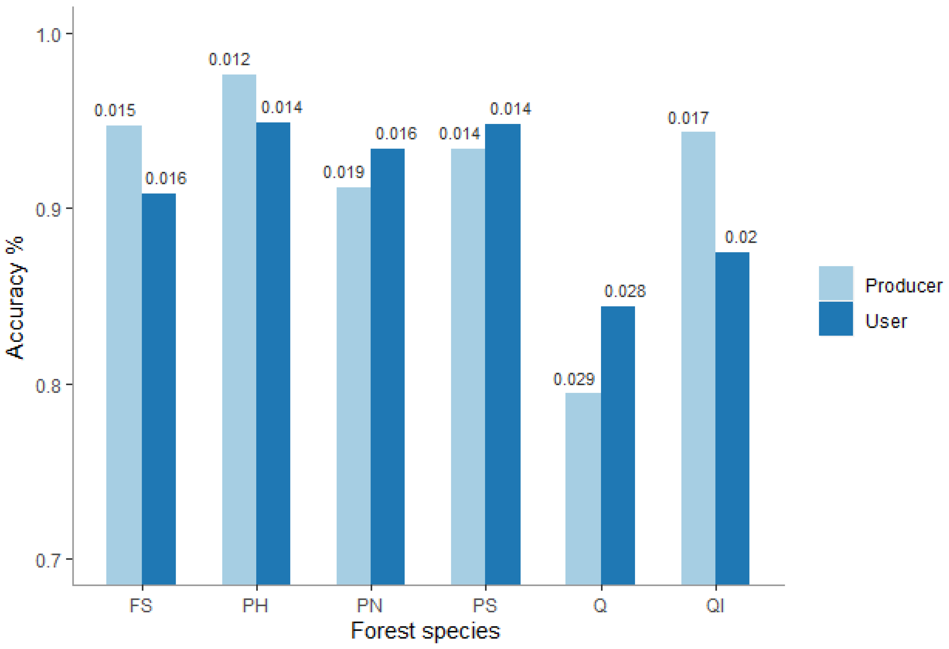
3.1. Accuracy Assessment

3.1.1. Forest Species Map Accuracy

The accuracy assessment of the original Landsat forest species map used the oob RF error (Table 2) and produced an overall accuracy of 88.77%. User’s and producer’s accuracies for most individual forest species were greater than 80% and even greater than 90% for some. User’s and producer’s accuracies were less for the Q, OB, and OC classes. The former showed a commission error of 23% due to confusion of this species with the OB class (see Table A2 in Appendix A), which also explains the OB omission error (23%). The OB class’s commission error (29%) is due to some of the points of this class erroneously classified as Q and FS. As for the OC class, it tends to be classified as some of the other Pinus spp. species and vice versa because of the similar spectral response among them. Nevertheless, the Landsat forest species map achieved an excellent overall accuracy of 98.8% for distinguishing between NF and the aggregation of all the forest species with producer’s accuracies of 92.9% and 99.7% and user’s accuracies of 98.1% and 98.8% for NF and the aggregation of forest classes, respectively.

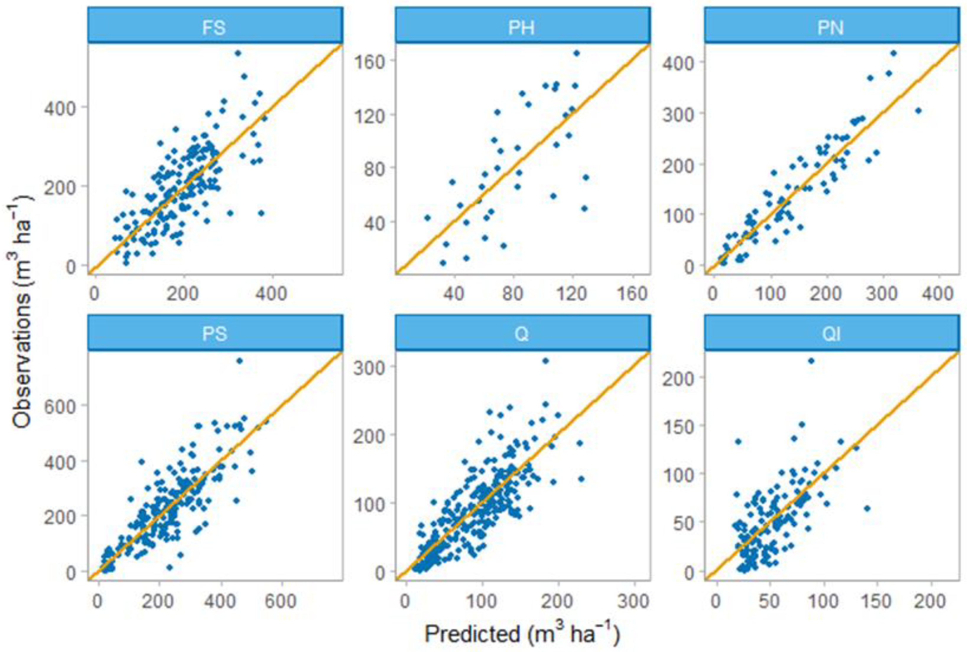
3.1.2. RF Volume Models

A graph of V predictions versus observations for SNFI plots showed that in general, most observations were located close to the 1:1 line, although a few observations exhibited a different tendency in the form of greater distances from this line (Figure 5). The lack of systematic error supports the previous MB inferential assumption that the RF model is essentially correct.

3.2. Uncertainty Assessment

3.2.1. The Effects of Uncertainty in the Landsat Forest Species Map on Area Estimates

SEs for the area estimates were generally less than 10% with the exception of PH and PN for which S E ( A ^   p   m a p k ) as percentages of estimates of the means reached 22.07% and 12.27%, respectively (Table 3). Greater SE estimates for areas for the latter two species are at least partially attributed to their less frequent occurrence among the six main forest species analyzed. These results indicate the overall variability in the Landsat forest species maps among the bootstrap iterations. The percentages of stable pixels were strongly positively correlated with the S E ( A ^   p   m a p k ) estimates. Among all species, more than 80% of the pixels were always classified as the same forest species, although for PH and PN, just 67% and 79% of the pixels remained stable. Regarding plot stability, among all species, nearly 80% of the field plots were in the forest portions of all 2000 Landsat forest species maps, one for each of the bootstrap iterations, and were therefore used for the calibration of V models. For individual species, PH exhibited the least plot stability with just 73% of the field plots selected for all 2000 Landsat forest species maps and with some plots selected for fewer than 50% of the maps. Excellent results were achieved for PS and Q for which the plot stabilities were nearly 100%. Although overall plot stabilities for these species were large, some field plots used to fit V models for these species were selected only a few times, particularly two plots that were selected for only about 40% of the maps. Generally, PH exhibited greater variability for area estimates and for plots selected to construct the RF V models, which was likely because this is an open grown forest species whose locations are more likely to be misclassified as non-forest.
A confusion matrix analysis for the Landsat forest species maps, constructed for the bootstrap iterations, was conducted using the RF oob error obtained with the pairs bootstrap resamples. The mean and the standard deviation of the accuracies of these maps over all iterations were estimated (Figure 6) with results similar to those for the original confusion matrix obtained for the original forest species map. Smaller user’s and producer’s accuracies were obtained for Q.

3.2.2. The Effects of Uncertainty in the Landsat Forest Species Map on Volume Estimates

Bootstrapping procedures were applied to assess the effects of map-to-map variability on the uncertainty of the V estimates for each of the most important forest species in La Rioja (Table 4). The results showed that the effects of map-to-map uncertainty were not negligible for any of the main forest species with S E ( V T   ^ p   m a p k ) % ranging from 3% to 22%. The uncertainties in the total V estimates resulting from the effects of uncertainty in the Landsat forest species map were greatest for PH (21.95%) and for QI (12.05%). The least S E ( V T   ^ p   m a p k ) % was achieved, from greatest to smallest, for FS, PS, and Q, as indicated by estimates of 3.17, 4.65, and 4.66%, respectively.

3.2.3. The Effects of Sampling Variability in the Model Calibration Dataset on Volume Estimates

Bootstrapping procedures were applied to assess the effects of plot-to-plot sampling variability for each of the most important forest species in La Rioja without consideration of the effects of map uncertainty. A total of 2000 iterations was sufficient for estimates of both means and SEs to stabilize (Figure 7). Overall, the V   ^ w   p l o t k estimates of the means were very similar to the μ ^ M B estimates (Table 5) with the greatest estimates for PS and FS and the least for PH and QI. The effects of plot-to-plot sampling variability on S E ( V T   ^ w   p l o t k ) % (as percentages of estimates of the total V) varied among the forest species, ranging from 2% to 11%. PH and QI were the forest species with more dispersion in the total V estimates as suggested by their larger S E ( V T   ^ w   p l o t k ) % values, 11.23% for the former and 9.07% for the latter. The smallest S E ( V T   ^ w   p l o t k ) % values, from smallest to greatest, were for PS, FS, and Q.

3.3. Total Uncertainty

The results (Table 6) revealed that the uncertainties in the V estimates were dominated by the effects of uncertainties in the Landsat forest species map as suggested by a greater S E ( V T   ^ p   m a p k ) relative to S E ( V T   ^ w   p l o t k ) obtained when considering only sampling variability associated with the model calibration data. When both sources of uncertainty were considered together, the SEs increased for all the forest species with increases greater than 5% for most species. Greater uncertainties were estimated for PH, with S E ( V T   ^ t o t a l k )   increasing from 11% to 25%, and for QI with increases from 9% to 15%.

4. Discussion

4.1. The Statistical Techniques

In this study, mean and total V estimates were inferred using an MB estimator based on RF predictions for the six main forest species of La Rioja (Spain). RF V models were constructed using SNFI field plot information and ALS data. To limit the prediction of V to pixels classified as one of the main forest species assessed, a forest species map was constructed using Landsat and auxiliary information and RF classification models. RF performed well with respect to both classification and prediction accuracy. Both RF models were calibrated with the default settings included in the R package RandomForest [43]. Balanced training samples were constructed to calibrate the RF classification, although RF is not known to be sensitive to the characteristics of the training sample [39]. An assessment of the effects of correlation among the ALS metrics on RF performance for volume prediction and therefore, procedures for selecting the most suitable variables would be appropriate [40,57].
Bootstrapping techniques were the lynchpin of this study and facilitated accounting for two sources of uncertainty: the uncertainty in the Landsat forest species map and the RF model prediction uncertainty resulting from the effects of sampling variability in the model training data. The similarity in the bootstrap estimates and the MB estimates indicates the lack of any substantial bias in the bootstrap procedure. Estimates of bootstrap means and standard errors stabilized by 2000 bootstrap iterations. However, this result should be generalized with caution and would better be considered a parameter that must be tuned for each forest species. As per Figure 6, the number of iterations necessary for estimates of the bootstrap means and standard errors to stabilize varied by forest species. Computer intensity will depend not only on the number of iterations but also on the size of the study area, with smaller study areas requiring less computation time. If a large number of iterations are necessary for a large study area, the development of the methodology could be conditional on access to a great deal of computationally capability. The workflow developed in this study was performed on a multi-processor Core i-7 6800 K box, with 12 cores and 64 GB memory because of the computational intensity involved. The cumulative effects of both sources of uncertainty were estimated with the effects of plot-to-plot sampling variability for the different maps assumed to be relatively constant. Apart from this assumption, the computational intensity associated with the methodology could become prohibitive, particularly if a large number of iterations were necessary to achieve stability in the estimates of means and standard errors. Nevertheless, the use of cloud-based platforms could overcome these difficulties providing the users with computing power at affordable prices.

4.2. Effects of Uncertainty in the Landsat Forest Species Map

The Landsat forest species map constructed for this study exhibited satisfactory accuracies considering the large number of forest species and their level of heterogeneity. Our results are in line with those reported by Fernández-Landa et al. [28] who used RF classification models to construct a map for PS and FS in a subset area of La Rioja of 16,000 ha. They reported user’s accuracies of 0.80 and 0.97 and producer’s accuracies of 0.97 and 0.89 for FS and PS, respectively. In their study, they claimed confusion between FS and OB as the main reason for the FS classification errors. Among the other forest species mapped, Q yielded the greatest commission errors coinciding with the results of other studies that mapped forest species using remotely sensed data in Mediterranean environments [58,59]. Despite the difficulty involved in mapping open forest species such as PH, the accuracies obtained for this study are in accordance with other studies conducted for Mediterranean species using multispectral information [60].
Uncertainty in the Landsat forest species map affects the V estimates in two manners: (1) it affects which plots are used to construct the species-specific V models, and (2) it affects the estimate of the area for each forest species that is multiplied by the estimate of the V mean. For the sake of simplicity, we assumed that the effects of plot-to-plot sampling variability in the model training data on V predictions for the different Landsat forest species maps to be relatively constant. Overall, the results justify this decision, because the differences in the field plots selected for the different Landsat forest species maps were relatively small. Hence, the results obtained suggest that the Landsat forest species map effects on area estimates are more important than the effects on field plot selection on RF model predictions. However, caution must be exercised with forest species in open woodlands such as PH, because the Landsat forest species map has a similar effect on both factors. On one hand, V models for PH were calibrated using a smaller calibration dataset (35 field plots) relative to the other forest species for which V models were calibrated. On the other hand, even though we refined the training dataset by removing the SNFI field plots that showed greater discrepancies, this dataset is characterized by a lack of location precision for its plot centers [28,61]. For species growing in open areas such as PH, this effect is exacerbated, resulting in a greater sampling variability (Figure 8) and increasing variance estimates [32].
An interesting pattern observed in this study is the strong positive relationship between pixel stability and SE for estimates of V totals. The results indicate that greater stability in the forest species classification produces less uncertainty in V estimates. In our study, we did not consider other sources of uncertainty such as tree measurement errors and ALS errors. However, both are expected to contribute very little to total uncertainty [62]. Nevertheless, if uncertainty in V estimates for smaller areas is desired, an approach accounting for residual uncertainty should be developed [63].
There was no positive relationship between species-specific pixel stabilities and accuracies obtained for the different Landsat forest species maps. Even though PH exhibited the largest variability in the pixels classified as such among the bootstrap iterations, it did not produce smaller accuracies. This is likely due to the location of the points used to train the RF classification models and therefore used to calculate the oob error, most of which were in dense forest areas. These points are less likely to be misclassified, although PH is a Mediterranean forest species occurring in open forest. These areas represent mixed pixels that were likely to be classified both as forest or non-forest, which could explain the larger PH classification variability. Uncertainty results at pixel scale facilitate analysis of the accuracy of the spatial distribution of V estimates and contribute to the identification of special patterns [12,56]. It is important to bear in mind that the reference data used to fit the RF classification models did not represent a probability sample but just an approximation. Although probability samples are not required for training data, future research could assess the effects on classification accuracy of probability-based samples of training data. Even though the RF oob error has been reported as a reliable accuracy measurement that can replace the use of an independent dataset [42], further research using a variety of datasets in different application scenarios would be appropriate [39].

4.3. Effects of Sampling Variability for the Model Calibration Datas

In this study, we only considered the uncertainty in the model predictions resulting from the effects of sampling variability. We did not include tree measurement errors for which the effects are generally regarded as negligible, thereby producing no meaningful adverse consequences [5]. Spatial correlation among pixel predictions was not included because for large contiguous area, distances between the vast majority of pairs of pixels are greater than the range of spatial correlation, thus, when averaging over all pairs of pixels, the overall effect is negligible [44]. Spatial correlation needs to be assessed in future research especially for smaller forest areas for which forest attributes are calculated. In addition, there were other sources of uncertainty involved in the V estimation framework such as the uncertainty associated with the V allometric model used in the SNFI and with the model linking plot-level V with ALS metrics. When these two sources of uncertainty are considered, uncertainty estimates are larger [12]. Sampling variability in the model calibration data produced SE% estimates in the range of 2–11% with greater values for PH and QI. Chirici et al. [64] estimated growing stock volume using NFI field plots and remotely sensed data (Landsat and SAR data) for a large area in Italy. Their SE estimates varied from 2% to 4%, although SE estimates were not reported for specific forest species. Irulappa-Pillai-Vijayakumar et al. [65] reported V estimates for a French region using NFI field plot data and remotely sensed data. They reported SE estimates of approximately 3% for oak V estimates and 5.76% for PS. For oak volume estimates, their SEs were slightly less than the SE of 5.46% for our study, although they did not consider the uncertainty of the forest species map.
The greater SEs for PH and QI are in accordance with the map uncertainty results as suggested by greater variability for PH and QI mapping. PH and QI are Mediterranean forest species that intermix with other vegetation types in complex patterns or in open woodlands. This complexity poses a challenge when using remote sensing-based classification methods in these kinds of environments as opposed to those in boreal forests [11,64]. A relationship between SEs for V totals and plot stabilities was not clearly observed as it was for pixel stability. That being said, it seems that there is a relationship between plot stability and the number of field plots used to calibrate the RF V models. Plot stabilities were less for PH and PN for which field plot sample sizes were smaller.

4.4. Total Uncertainty

Many studies have reported large area V estimates, even at a country level, using models and remotely sensed data [21,64,66]. These studies have demonstrated the potential of assessing forest resources using different sources of information already acquired and therefore posing an opportunity to replicate the methodology in other countries with well-established NFI programs. However, the results of our study demonstrated that if similar approaches are to be replicated, it is necessary to include the uncertainty of the forest species map used. Uncertainty results can be underestimated when the uncertainty of the forest species map is ignored in the modeling approach. This is particularly relevant for the V estimates for forest species: (1) for less representative species such as PN, incorporating the effects of map uncertainty increased SE% from 2.94% to 9.19%; and (2) for Mediterranean forest species occurring in open areas such as PH, incorporation of the effects of map uncertainty increase SE% from 11.23% to 24.66%. Further work is recommended to construct uncertainty maps at a pixel scale that represents the spatial distributions of the accumulated sources of uncertainty considered. Such maps would be key to distinguishing uncertainties between site conditions and estimated volume levels [12].

4.5. Operational Consequences

This study is unique because of our approach to propagating uncertainty to account for the effects of uncertainty in the map of the spatial distribution of the main forest species estimated from Landsat and from the effects of sampling variability on RF V model predictions. Even though we used a different approach for constructing the forest map than the SNFM, the results are relevant for the SNFI. On one hand, although the SNFI used a forest map constructed by photo-interpretation, it could also have potential errors that might affect the V estimates. On the other hand, until now, national V estimates have been sample-based, but because of the economic crisis, the number of field plots has been reduced [10]. Nevertheless, an appropriate use of remotely sensed data could guarantee that accuracy is not lost in forest attribute predictions, even if the number of field plots was reduced [67], although it is crucial to account for the time interval between field data and remotely sensed data used. However, if NFI plots are to be established only in the forest portion of a remote sensing-based forest map, then the uncertainty associated with the map should be considered. Otherwise, countries will underestimate uncertainty and fail to comply with the IPCC good practice guidelines [24].

5. Conclusions

Our study assessed the effects of uncertainty in a forest species map involved in the selection of the field plots used to calibrate the volume models and in the estimation process on the uncertainty of large area volume estimates. Five conclusions were drawn from the study: (1) the effects of uncertainty in the forest species map on the uncertainty of large area volume estimates are not negligible, and ignoring the effects could jeopardize the reliability of the forest volume estimates; (2) overall, the effects of uncertainty in the forest species map on area estimates were greater than the effects of uncertainty in the map on the selection of field plots used to calibrate the RF volume prediction model; (3) the effects of the forest species map uncertainty increased for open forest species or less representative forest species; (4) bootstrapping estimates demonstrated the suitability of this technique to accommodate the effects of uncertainty from more than one source; and (5) the results are relevant for countries that use a remote sensing-based forest/non-forest map to guide the establishment of field plots. Further work in a variety of forest environments to assess whether the conclusions can be generalized beyond Mediterranean environments is recommended.

Author Contributions

Conceptualization, J.E., R.E.M. and A.F.-L.; methodology, J.E., R.E.M. and A.F.-L.; software, J.E.; formal analysis, J.E., R.E.M., A.F.-L., J.L.T. and M.M.; resources, J.E., A.F.-L. and J.L.T.; data curation, J.E., A.F.-L. and J.L.T.; writing—original draft preparation, J.E., R.E.M., A.F.-L., J.L.T. and M.M.; writing—review and editing, J.E., R.E.M., A.F.-L., J.L.T. and M.M.; visualization, J.E.; funding acquisition, M.M. All authors have read and agreed to the published version of the manuscript.

Funding

First author is supported by a pre-doctoral contract co-funded by Universidad Politécnica de Madrid and Agresta S.Coop.

Acknowledgments

We are grateful to the National Geographic Institute from Spain and thank to the Spanish National Forest Inventory for providing free access to ALS data and forest inventory information.

Conflicts of Interest

The authors declare no conflict of interest.

Abbreviations

AbbreviationFull Description
ALSAirborne laser scanning
crrALS canopy relief ratio
cvALS height coefficient of variation
DBHDiameter at breast height
FSFagus sylvatica
IPCCIntergovernmental Panel on Climate Change
iqALS height interquartile range
kurtoALS height kurtosis
lfccForest canopy cover
MBModel-based
MSEMean square error
NBRNormalized Burn Ratio
NDMINormalized Difference Moisture Index
NDVINormalized Difference Vegetation Index
NFINational Forest Inventory
NIRNear infrared
OBOther broadleaves
OCOther coniferous
oobOut-of-bag
p1-p99ALS percentiles (ranging from the 1st to 99th percentile)
PHPinus halepensis
PNPinus nigra
PSPinus sylvestris
QQuercus faginea or Quercus pyrenaica
QIQuercus ilex
RFRandom forest
RMSERoot mean square error
rRMSERelative root mean square error
RSRemote sensing
SEStandard error
SNFISpanish National Forest Inventory
SNFMSpanish National Forest Map
stdevALS height standard deviation
TMThematic Mapper
VMean volume per hectare
variaALS height variance

Appendix A

Table A1. Summary of the V models using 2010 airborne laser scanning (ALS) data and SNFI field plots for the six main forest species of La Rioja (Spain). Measures of predictive accuracy were obtained from the out-of-bag (oob) internal error derived from the RF models.
Forest Species *% Variance ExplainedMSE (m3/ha)RMSE (m3/ha)rRMSE (%)
FS52.624081.8463.8933.27
PH44.37 973.2431.2038.72
PN85.641279.0135.7625.97
PS69.265665.1375.2733.43
Q64.471084.8532.9436.47
QI36.38 769.5227.7452.43
* FS: Fagus sylvatica; PH: Pinus halepensis; PN: Pinus nigra; PS: Pinus sylvestris; Q: Quercus pyrenaica/faginea; QI: Quercus ilex. Note: MSE: mean square error; RMSE: root mean square error, and rRMSE: relative root mean square error.
Table A2. Out-of-bag confusion matrix derived from the RF classification model fitted to construct a forest species map for the study area. Columns represent true classes, while rows represent the classifier’s predictions.
Forest Species *NFFSPHPNPSQQIOBOC
NF15801100001
FS01461310123
PH10104001001
PN02310006100
PS01008451360
Q30114128013
QI21019689125
OB00002071610
OC6211074297
* NF: Non-forest; FS: Fagus sylvatica; PH: Pinus halepensis; PN: Pinus nigra; PS: Pinus sylvestris; Q: Quercus pyrenaica/faginea; QI: Quercus ilex; OB: “Other broadleaves” (OB) and OC: “Other coniferous”.

References

  1. Food and Agriculture Organizations of the United Nations. State of Europe’s Forests 2015 Report. 2015. Available online: https://foresteurope.org/state-europes-forests-2015-report/ (accessed on 12 October 2020).
  2. McRoberts, R.E.; Tomppo, E.O.; Næsset, E. Advances and emerging issues in national forest inventories. Scand. J. For. Res. 2010, 25, 368–381. [Google Scholar] [CrossRef]
  3. Vidal, C.; Alberdi, I.; Redmond, J.; Vestman, M.; Lanz, A.; Schadauer, K. The role of European National Forest Inventories for international forestry reporting a Legally Binding Agreement. Ann. For. Sci. 2016, 73, 793–806. [Google Scholar] [CrossRef] [Green Version]
  4. Alberdi, I.; Vallejo, R.; Álvarez-González, J.G.; Condés, S.; González-Ferreiro, E.; Guerrero, S.; Hernández, L.; Martínez-Jauregui, M.; Montes, F.; Oliveira, N.; et al. The multi-objective Spanish National Forest Inventory. For. Syst. 2017, 26, 1–17. [Google Scholar] [CrossRef]
  5. McRoberts, R.E.; Westfall, J.A. Propagating uncertainty through individual tree volume model predictions to large-area volume estimates. Ann. For. Sci. 2016, 73, 625–633. [Google Scholar] [CrossRef] [Green Version]
  6. Grafstörm, A.; Saarela, S.; Ene, L. Efficient sampling strategies for forest inventories by spreading the sample in auxiliary space. Can. J. For. Res. 2014, 44, 1156–1164. [Google Scholar] [CrossRef]
  7. McRoberts, R.E.; Cohen, W.B.; Erik, N.; Stehman, S.V.; Tomppo, E.O. Using remotely sensed data to construct and assess forest attribute maps and related spatial products. Scand. J. For. Res. 2010, 25, 340–367. [Google Scholar] [CrossRef]
  8. McRoberts, R.E.; Næsset, E.; Sannier, C.; Stehman, S.V.; Tomppo, E.O. Remote sensing support for the gain-loss approach for greenhouse gas inventories. Remote Sens. 2020, 12, 1891. [Google Scholar] [CrossRef]
  9. Tomppo, E.; Gschwantner, T.; Lawrence, M.; McRoberts, R.E. National Forest Inventories: Pathways for Common Reporting; Springer: Dordrecht, The Netherlands, 2010; ISBN 978-90-481-3233-1. [Google Scholar]
  10. Alberdi, I.; Cañellas, I.; Vallejo Bombín, R. The Spanish National Forest Inventory: History, development, challenges and perspectives. Pesqui. Florest. Bras. 2017, 37, 361. [Google Scholar] [CrossRef]
  11. Gomez, C.; Alejandro, P.; Hermosilla, T.; Montes, F.; Pascual, C.; Ruiz, L.Á.; Alvarez-taboada, F.; Tanase, M.A.; Valbuena, R. Remote sensing for the Spanish forests in the 21 st century: A review of advances, needs, and opportunities. For. Syst. 2019, 28, eR001. [Google Scholar]
  12. Saarela, S.; Wästlund, A.; Holmström, E.; Mensah, A.A.; Holm, S.; Nilsson, M.; Fridman, J.; Ståhl, G. Mapping aboveground biomass and its prediction uncertainty using LiDAR and field data, accounting for tree-level allometric and LiDAR model errors. For. Ecosyst. 2020, 7, 43. [Google Scholar] [CrossRef]
  13. McRoberts, R.E.; Tomppo, E.O. Remote sensing support for national forest inventories. Remote Sens. Environ. 2007, 110, 412–419. [Google Scholar] [CrossRef]
  14. White, J.C.; Coops, N.C.; Wulder, M.A.; Vastaranta, M.; Hilker, T.; Tompalski, P. Remote Sensing Technologies for Enhancing Forest Inventories: A Review. Can. J. Remote Sens. 2016, 42, 619–641. [Google Scholar] [CrossRef] [Green Version]
  15. Ståhl, G.; Saarela, S.; Schnell, S.; Holm, S.; Breidenbach, J.; Healey, S.P.; Patterson, P.L.; Magnussen, S.; Næsset, E.; McRoberts, R.E.; et al. Use of models in large-area forest surveys: Comparing model-assisted, model-based and hybrid estimation. For. Ecosyst. 2016, 3, 5. [Google Scholar] [CrossRef] [Green Version]
  16. McRoberts, R.E.; Moser, P.; Zimermann Oliveira, L.; Vibrans, A.C. A general method for assessing the effects of uncertainty in individual-tree volume model predictions on large-area volume estimates with a subtropical forest illustration. Can. J. For. Res. 2014, 45, 44–51. [Google Scholar] [CrossRef]
  17. McRoberts, R.E.; Næsset, E.; Gobakken, T. Estimation for inaccessible and non-sampled forest areas using model-based inference and remotely sensed auxiliary information. Remote Sens. Environ. 2014, 154, 226–233. [Google Scholar] [CrossRef]
  18. Hansen, M.H.; Madow, W.G.; Tepping, B.J. An evaluation of model-dependent and probability-sampling inferences in sample surveys. J. Am. Stat. Assoc. 1983, 78, 776–793. [Google Scholar] [CrossRef]
  19. Royall, R.M.; Herson, J. Robust Estimation in Finite Populations I. J. Am. Stat. Assoc. 1973, 68, 880–889. [Google Scholar] [CrossRef]
  20. Shettles, M.; Temesgen, H.; Gray, A.N.; Hilker, T. Comparison of uncertainty in per unit area estimates of aboveground biomass for two selected model sets. For. Ecol. Manag. 2015, 354, 18–25. [Google Scholar] [CrossRef]
  21. Urbazaev, M.; Thiel, C.; Cremer, F.; Dubayah, R.; Migliavacca, M.; Reichstein, M.; Schmullius, C. Estimation of forest aboveground biomass and uncertainties by integration of field measurements, airborne LiDAR, and SAR and optical satellite data in Mexico. Carbon Balance Manag. 2018, 13, 1–12. [Google Scholar] [CrossRef] [Green Version]
  22. Rodríguez-Veiga, P.; Saatchi, S.; Tansey, K.; Balzter, H. Magnitude, spatial distribution and uncertainty of forest biomass stocks in Mexico. Remote Sens. Environ. 2016, 183, 265–281. [Google Scholar] [CrossRef] [Green Version]
  23. Li, X.; Messina, J.P.; Moore, N.J.; Fan, P.; Shortridge, A.M. MODIS land cover uncertainty in regional climate simulations. Clim. Dyn. 2017, 49, 4047–4059. [Google Scholar] [CrossRef] [Green Version]
  24. IPCC. Volume 4: Agriculture, Forestry and other land use. In Refinement to the 2006 IPCC Guidelines for National Greenhouse Gas Inventories; Calvo Buendia, E., Tanabe, K., Kranjc, A., Baasansuren, J., Fukuda, M., Ngarize, S., Osako, A., Pyrozhenko, Y., Shermanau, P., Federici, S., Eds.; IPCC: Geneva, Switzerland, 2019; Available online: https://www.ipcc-nggip.iges.or.jp/public/2019rf/index.html (accessed on 12 October 2020).
  25. Bravo, F.; Guijarro, M.; Cámara, A.; Balteiro, L.D.; Fernández-Rebollo, P.; Pajares, J.A.; Pemán, J.; Ruiz-Peinado, R. Informe de Situación de los bosques y sector forestal en España—ISFE 2017. Sociedad Española de Ciencias Forestales. 2017. Available online: http://secforestales.org/sites/default/files/archivos/7cfe_avance_isfe_final.pdf (accessed on 12 October 2020).
  26. Cuarto Inventario Forestal Nacional La Rioja. Edited by Ministerio de Agricultura, Alimentación y Medio Ambiente. Available online: https://docplayer.es/4459716-Cuarto-inventario-forestal-nacional-la-rioja.html (accessed on 12 October 2020).
  27. Álvarez-González, J.G.; Cañellas, I.; Alberdi, I.; Gadow, K.V.; Ruiz-González, A.D. National Forest Inventory and forest observational studies in Spain: Applications to forest modeling. For. Ecol. Manag. 2014, 316, 54–64. [Google Scholar] [CrossRef]
  28. Fernández-Landa, A.; Fernández-Moya, J.; Tomé, J.L.; Algeet-Abarquero, N.; Guillén-Climent, M.L.; Vallejo, R.; Sandoval, V.; Marchamalo, M. High resolution forest inventory of pure and mixed stands at regional level combining National Forest Inventory field plots, Landsat, and low density lidar. Int. J. Remote Sens. 2018, 39, 4830–4844. [Google Scholar] [CrossRef]
  29. Gorelick, N.; Hancher, M.; Dixon, M.; Ilyushchenko, S.; Thau, D.; Moore, R. Google Earth Engine: Planetary-scale geospatial analysis for everyone. Remote Sens. Environ. 2017, 202, 18–27. [Google Scholar] [CrossRef]
  30. McGaughey, R.; Forester, R.; Carson, W. Fusing LIDAR data, photographs, and other data using 2D and 3D visualization techniques. Proc. Terrain Data Appl. Vis. Connect. 2003, 28–30, 16–24. [Google Scholar]
  31. Næsset, E.; Bollandsås, O.M.; Gobakken, T.; Solberg, S.; McRoberts, R.E. The effects of field plot size on model-assisted estimation of aboveground biomass change using multitemporal interferometric SAR and airborne laser scanning data. Remote Sens. Environ. 2015, 168, 252–264. [Google Scholar] [CrossRef]
  32. Saarela, S.; Grafström, A.; Ståhl, G.; Kangas, A.; Holopainen, M.; Tuominen, S.; Nordkvist, K.; Hyyppä, J. Model-assisted estimation of growing stock volume using different combinations of LiDAR and Landsat data as auxiliary information. Remote Sens. Environ. 2015, 158, 431–440. [Google Scholar] [CrossRef]
  33. McRoberts, R.E.; Chen, Q.; Domke, G.M.; Ståhl, G.; Saarela, S.; Westfall, J.A. Hybrid estimators for mean aboveground carbon per unit area. For. Ecol. Manag. 2016, 378, 44–56. [Google Scholar] [CrossRef]
  34. Breiman, L. Random Forests. Mach. Learn. 2001, 45, 5–32. [Google Scholar] [CrossRef] [Green Version]
  35. Shataee, S.; Kalbi, S.; Fallah, A.; Pelz, D. Forest attribute imputation using machine-learning methods and ASTER data: Comparison of k-NN, SVR and random forest regression algorithms. Int. J. Remote Sens. 2012, 33, 6254–6280. [Google Scholar] [CrossRef]
  36. Penner, M.; Pitt, D.G.; Woods, M.E. Parametric vs. nonparametric LiDAR models for operational forest inventory in boreal Ontario. Can. J. Remote Sens. 2013, 39, 426–443. [Google Scholar]
  37. Rodriguez-Galiano, V.F.; Chica-Rivas, M. Evaluation of different machine learning methods for land cover mapping of a Mediterranean area using multi-seasonal Landsat images and Digital Terrain Models. Int. J. Digit. Earth 2012, 7, 492–509. [Google Scholar] [CrossRef]
  38. Grinand, C.; Rakotomalala, F.; Gond, V.; Vaudry, R.; Bernoux, M.; Vieilledent, G. Estimating deforestation in tropical humid and dry forests in Madagascar from 2000 to 2010 using multi-date Landsat satellite images and the random forests classifier. Remote Sens. Environ. 2013, 139, 68–80. [Google Scholar] [CrossRef]
  39. Belgiu, M.; Drăguţ, L. Random forest in remote sensing: A review of applications and future directions. ISPRS J. Photogramm. Remote Sens. 2016, 114, 24–31. [Google Scholar] [CrossRef]
  40. Moser, P.; Vibrans, A.C.; McRoberts, R.E.; Næsset, E.; Gobakken, T.; Chirici, G.; Mura, M.; Marchetti, M. Methods for variable selection in LiDAR-assisted forest inventories. Forestry 2016, 90, 112–124. [Google Scholar] [CrossRef] [Green Version]
  41. Navarro, J.A.; Algeet, N.; Fernández-Landa, A.; Esteban, J.; Rodríguez-Noriega, P.; Guillén-Climent, M.L. Integration of UAV, Sentinel-1, and Sentinel-2 data for mangrove plantation aboveground biomass monitoring in Senegal. Remote Sens. 2019, 11, 77. [Google Scholar] [CrossRef] [Green Version]
  42. Rodriguez-Galiano, V.F.; Ghimire, B.; Rogan, J.; Chica-Olmo, M.; Rigol-Sanchez, J.P. An assessment of the effectiveness of a random forest classifier for land-cover classification. ISPRS J. Photogramm. Remote Sens. 2012, 67, 93–104. [Google Scholar] [CrossRef]
  43. Liaw, A.; Wiener, M. Classification and Regression by randomForest. R News 2002, 2, 18–22. [Google Scholar]
  44. McRoberts, R.E.; Næsset, E.; Gobakken, T.; Chirici, G.; Condés, S.; Hou, Z.; Saarela, S.; Chen, Q.; Ståhl, G.; Walters, B.F. Assessing components of the model-based mean square error estimator for remote sensing assisted forest applications. Can. J. For. Res. 2018, 48, 642–649. [Google Scholar] [CrossRef]
  45. Condés, S.; McRoberts, R.E. Updating national forest inventory estimates of growing stock volume using hybrid inference. For. Ecol. Manag. 2017, 400, 48–57. [Google Scholar] [CrossRef]
  46. Hou, Z.; Xu, Q.; McRoberts, R.E.; Greenberg, J.A.; Liu, J.; Heiskanen, J.; Pitkänen, S.; Packalen, P. Effects of temporally external auxiliary data on model-based inference. Remote Sens. Environ. 2017, 198, 150–159. [Google Scholar] [CrossRef]
  47. McRoberts, R.E.; Magnussen, S.; Tomppo, E.O.; Chirici, G. Parametric, bootstrap, and jackknife variance estimators for the k-Nearest Neighbors technique with illustrations using forest inventory and satellite image data. Remote Sens. Environ. 2011, 115, 3165–3174. [Google Scholar] [CrossRef]
  48. Hou, Z.; McRoberts, R.E.; Ståhl, G.; Packalen, P.; Greenberg, J.A.; Xu, Q. How much can natural resource inventory benefit from finer resolution auxiliary data? Remote Sens. Environ. 2018, 209, 31–40. [Google Scholar] [CrossRef]
  49. Efron, B.; Tibshirani, R.J. An Introduction to the Bootstrap; Chapman and Hall: New York, NY, USA, 1994. [Google Scholar]
  50. Liu, R. Bootstrap Procedures under some Non-I.I.D. Models. Ann.Stat. 1988, 16, 1696–1708. [Google Scholar] [CrossRef]
  51. Carpenter, J.; Bithell, J. Bootstrap confidence intervals: When, which, what? A practical guide for medical statisticians. Stat. Med. 2000, 19, 1141–1164. [Google Scholar] [CrossRef]
  52. Diaconis, P.; Efron, B. Computer-Intensive Methods in Statistics. Sci. Am. 1983, 248, 116–130. [Google Scholar] [CrossRef]
  53. Ranalli, M.G.; Mecatti, F. Comparing Recent Approaches For Bootstrapping Sample Survey Data: A First Step Towards A Unified Approach. Proc. Surv. Res. Methods Sect. Am. Stat. Assoc. 2012, 4088–4099. Available online: http://boa.unimib.it/retrieve/handle/10281/41947/62652/Ranalli_Mecatti_Proc2013.pdf (accessed on 12 October 2020).
  54. Flachaire, E. Bootstrapping heteroskedastic regression models: Wild bootstrap vs. pairs bootstrap. Comput. Stat. Data Anal. 2005, 49, 361–376. [Google Scholar] [CrossRef] [Green Version]
  55. Freedman, D.A. Bootstrapping Regression Models. Ann. Stat. 1981, 6, 1218–1228. [Google Scholar] [CrossRef]
  56. Esteban, J.; McRoberts, R.E.; Fernández-Landa, A.; Tomé, J.L.; Næsset, E. Estimating forest volume and biomass and their changes using random forests and remotely sensed data. Remote Sens. 2019, 11, 1944. [Google Scholar] [CrossRef] [Green Version]
  57. Domingo, D.; Alonso, R.; de la Riva, J.; Lamelas, M.T.; Rodríguez, F.; Montealegre, A.L. Temporal Transferability of Pine Forest Attributes Modeling Using Low-Density Airborne Laser Scanning Data. Remote Sens. 2019, 11, 261. [Google Scholar] [CrossRef] [Green Version]
  58. Rodriguez-Galiano, V.; Chica-Olmo, M. Land cover change analysis of a Mediterranean area in Spain using different sources of data: Multi-seasonal Landsat images, land surface temperature, digital terrain models and texture. Appl. Geogr. 2012, 35, 208–218. [Google Scholar] [CrossRef]
  59. Stavrakoudis, D.G.; Dragozi, E.; Gitas, I.Z.; Karydas, C.G. Decision Fusion Based on Hyperspectral and Multispectral Satellite Imagery for Accurate Forest Species Mapping. Remote Sens. 2014, 6, 6897–6928. [Google Scholar] [CrossRef] [Green Version]
  60. Pesaresi, S.; Mancini, A.; Quattrini, G.; Casavecchia, S. Mapping Mediterranean Forest Plant Associations and Habitats with Functional Principal Component Analysis Using Landsat 8 NDVI Time Series. Remote Sens. 2020, 12, 1132. [Google Scholar] [CrossRef] [Green Version]
  61. Valbuena, R.; Mauro, F.; Rodriguez-Solano, R.; Manzanera, J.A. Accuracy and precision of GPS receivers under forest canopies in a mountainous environment. Span. J. Agric. Res. 2013, 8, 1047. [Google Scholar] [CrossRef]
  62. Chen, Q.; Vaglio Laurin, G.; Valentini, R. Uncertainty of remotely sensed aboveground biomass over an African tropical forest: Propagating errors from trees to plots to pixels. Remote Sens. Environ. 2015, 160, 134–143. [Google Scholar] [CrossRef]
  63. Breidenbach, J.; Astrup, R. Small area estimation of forest attributes in the Norwegian National Forest Inventory. Eur. J. For. Res. 2012, 131, 1255–1267. [Google Scholar] [CrossRef]
  64. Chirici, G.; Giannetti, F.; McRoberts, R.E.; Travaglini, D.; Pecchi, M.; Maselli, F.; Chiesi, M.; Corona, P. Wall-to-wall spatial prediction of growing stock volume based on Italian National Forest Inventory plots and remotely sensed data. Int. J. Appl. Earth Obs. Geoinf. 2020, 84, 101959. [Google Scholar] [CrossRef]
  65. Irulappa-Pillai-Vijayakumar, D.B.; Renaud, J.P.; Morneau, F.; McRoberts, R.E.; Vega, C. Increasing precision for French forest inventory estimates using the k-NN technique with optical and photogrammetric data and model-assisted estimators. Remote Sens. 2019, 11, 991. [Google Scholar] [CrossRef] [Green Version]
  66. Maselli, F.; Chiesi, M.; Mura, M.; Marchetti, M.; Corona, P.; Chirici, G. Combination of optical and LiDAR satellite imagery with forest inventory data to improve wall-to-wall assessment of growing stock in Italy. Int. J. Appl. Earth Obs. Geoinf. 2014, 26, 377–386. [Google Scholar] [CrossRef]
  67. McRoberts, R.E.; Næsset, E.; Gobakken, T. Inference for lidar-assisted estimation of forest growing stock volume. Remote Sens. Environ. 2013, 128, 268–275. [Google Scholar] [CrossRef]
Figure 1. La Rioja study area and distribution of the main forest species based on the Spanish National Forest Map. ETRS89/UTM zone 30N (N-E) (EPSG: 3042). The blue polygon in the lower right corner depicts the location of the study area in north central Spain.
Remotesensing 12 03360 g001
Figure 2. Workflow diagram of the processing steps conducted to account for the sources of uncertainty involved in the volume estimation.
Remotesensing 12 03360 g002
Figure 3. Wild bootstrapping scheme conducted in this study to account for the effects of plot-to-plot sampling variability in the model training data, ignoring uncertainty in the Landsat forest species map.
Remotesensing 12 03360 g003
Figure 4. Wild and pairs bootstrapping schemes used to account for uncertainty in the Landsat forest species map.
Remotesensing 12 03360 g004
Figure 5. Volume reference values for each of the field plots, used to construct the different RF models, versus their predictions. Note: FS: Fagus sylvatica; PH: Pinus halepensis; PN: Pinus nigra; PS: Pinus sylvestris; Q: Quercus pyrenaica/faginea; QI: Quercus ilex. Orange line represents the 1:1 line.
Remotesensing 12 03360 g005
Figure 6. Mean and the standard error estimates (number at the top of each bar) of the accuracies (from 0 to 1) of the Landsat forest species maps over all the iterations for the main forest species of La Rioja. Note: FS: Fagus sylvatica; PH: Pinus halepensis; PN: Pinus nigra; PS: Pinus sylvestris; Q: Quercus pyrenaica/faginea; QI: Quercus ilex.
Remotesensing 12 03360 g006
Figure 7. Estimates for means and standard errors for each bootstrap iteration and forest species analyzed. Note: FS: Fagus sylvatica; PH: Pinus halepensis; PN: Pinus nigra; PS: Pinus sylvestris; Q: Quercus pyrenaica/faginea; QI: Quercus ilex.
Remotesensing 12 03360 g007
Figure 8. Examples of SNFI field plots used for V prediction purposes for PH not included in 100% of the total bootstrap iterations conducted to assess plot-to-plot variability. Yellow squares represent population units of cell size of 25 × 25 m.
Remotesensing 12 03360 g008
Table 1. Statistics for mean volume (m3/ha) obtained from the Spanish National Forest Inventory (SNFI) field plots classified as forest according to the Landsat forest species map and used for the construction of the V models.
Forest Species *Number of SNFI PlotsMeanStandard DeviationMinimumMaximum
FS182192.6293.075.89530.81
PH3580.5842.449.06164.24
PN82137.6994.963.71415.36
PS199225.12136.102.53756.76
Q27290.3155.361.44305.75
QI13652.9134.990.00215.51
* FS: Fagus sylvatica; PH: Pinus halepensis; PN: Pinus nigra; PS: Pinus sylvestris; Q: Quercus pyrenaica/faginea; QI: Quercus ilex.
Table 2. Out-of-bag confusion matrix estimated from the random forest (RF) classification model fitted to construct a forest species map for the study area.
Forest Species *User’s Accuracy (%)Commission Error (%)Producer’s Accuracy (%)Omission Error (%)
NF982937
FS9558813
PH973946
PN8911937
PS937964
Q77238416
QI9198416
OB71297723
OC81198812
* NF: Non-forest; FS: Fagus sylvatica; PH: Pinus halepensis; PN: Pinus nigra; PS: Pinus sylvestris; Q: Quercus pyrenaica/faginea; QI: Quercus ilex; OB: “Other broadleaves” (OB) and OC: “Other coniferous”.
Table 3. Area estimates (ha) and pixel and plot stabilities for the main forest species in La Rioja.
Forest Species *Area EstimatesStandard ErrorsStability
A ^ k (ha)   A ^   p   m a p k (ha) S E ( A   ^ p   m a p k ) (ha) S E ( A ^   p   m a p k )   (%)% of Stable Pixels% of Stable Plots
See Footnote (**)Equation (2) Equation (3)Equations (2) and (3)
FS2.10 × 1042.24 × 104552.662.4794.20100.00
PH1.09 × 1040.97 × 1042132.2622.0766.8572.97
PN0.67 × 1040.63 × 104779.1212.2779.5286.59
PS1.79 × 1041.86 × 1041243.836.6792.0196.48
Q5.51 × 1045.06 × 1042664.665.2783.5495.96
QI3.53 × 1043.61 × 1043202.958.8484.5186.76
* FS: Fagus sylvatica; PH: Pinus halepensis; PN: Pinus nigra; PS: Pinus sylvestris; Q: Quercus pyrenaica/faginea; QI: Quercus ilex. ** Calculated as the product of pixel size and the number of pixels classified as species k in the original Landsat forest species map.
Table 4. Volume estimates and standard errors based on uncertainty in the Landsat forest species map.
Forest Species *Mean Volume (m3/ha)Total Volume (m3)
V p   m a p k ^   S E ( V   ^ p   m a p k )   V T   ^ p   m a p k S E ( V T   ^ p   m a p k ) S E ( V T   ^ p   m a p k ) (%)
Equation (10)Equation (11)Equation (12)Equation (13)Equations (12) and (13)
FS204.055.464.57 × 1061.45 × 1053.17
PH67.387.910.65 × 1061.42 × 10521.95
PN144.058.750.91 × 1060.79 × 1058.71
PS216.288.624.02 × 1061.87 × 1054.65
Q70.502.803.56 × 1061.66 × 1054.66
QI 44.634.101.62 × 1061.95 × 10512.05
* FS: Fagus sylvatica; PH: Pinus halepensis; PN: Pinus nigra; PS: Pinus sylvestris; Q: Quercus pyrenaica/faginea; QI: Quercus ilex.
Table 5. Volume estimates and standard errors based on sampling variability in model calibration dataset.
Forest Species *Mean Volume (m3/ha)Total Volume (m3)
μ ^ M B   V   ^ w   p l o t k   S E ( V   ^ w   p l o t k ) (%) V T ^   V T   ^ w   p l o t k   S E ( V T   ^ w   p l o t k ) S E ( V T   ^ w   p l o t k ) (%)
Equation (1)Equation (5)Equation (6)See Footnote (**)Equation (7)Equation (8)Equations (7) and (8)
FS203.70204.295.024.28 × 1064.29 × 1061.06 × 1052.46
PH61.5266.497.470.67 × 1060.73 × 1060.82 × 10511.23
PN146.96144.224.250.99 × 1060.97 × 1060.28 × 1052.94
PS223.08220.435.223.99 × 1063.95 × 1060.94 × 105 2.37
Q70.8472.432.063.90 × 1063.99 × 1061.13 × 1052.84
QI43.2744.464.031.53 × 1061.57 × 1061.43 × 1059.07
* FS: Fagus sylvatica; PH: Pinus halepensis; PN: Pinus nigra; PS: Pinus sylvestris; Q: Quercus pyrenaica/faginea; QI: Quercus ilex. ** Calculated as the product of species-specific area, from original Landsat forest species map, and mean V based on plots from SNFI field dataset located within area classified as the species.
Table 6. Uncertainties in total volume estimates for the main forest species of La Rioja.
Forest Species *Uncertainty in the Landsat Forest Species MapSampling Variability in Model Calibration DataTotal Uncertainty
S E ( V T   ^ p   m a p k )   (%) S E ( V T   ^ w   p l o t k ) (%) S E ( V T   ^ t o t a l k ) (%)
Equations (12) and (13)Equations (7) and (8)Equation (14)
FS3.172.464.01
PH21.9511.2324.66
PN8.712.949.19
PS4.652.375.22
Q4.662.845.46
QI12.059.0715.08
* FS: Fagus sylvatica; PH: Pinus halepensis; PN: Pinus nigra; PS: Pinus sylvestris; Q: Quercus pyrenaica/faginea; QI: Quercus ilex.
Publisher’s Note: MDPI stays neutral with regard to jurisdictional claims in published maps and institutional affiliations.

