Variations in Spectral Signals of Heavy Metal Contamination in Mine Soils Controlled by Mineral Assemblages


Abstract
:1. Introduction
2. Materials and Methods
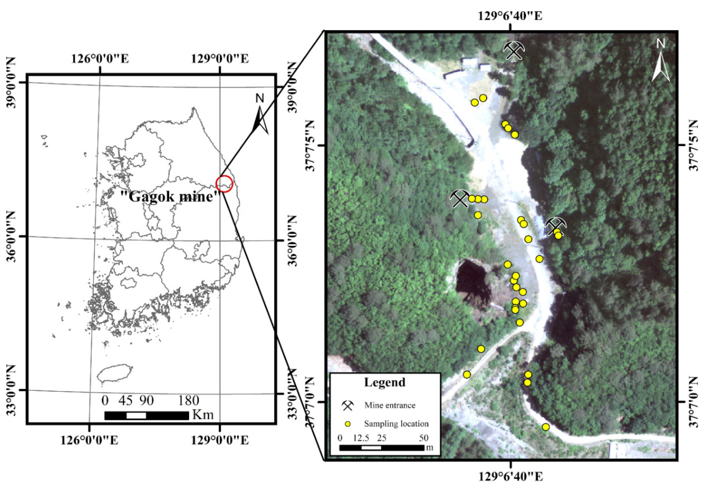
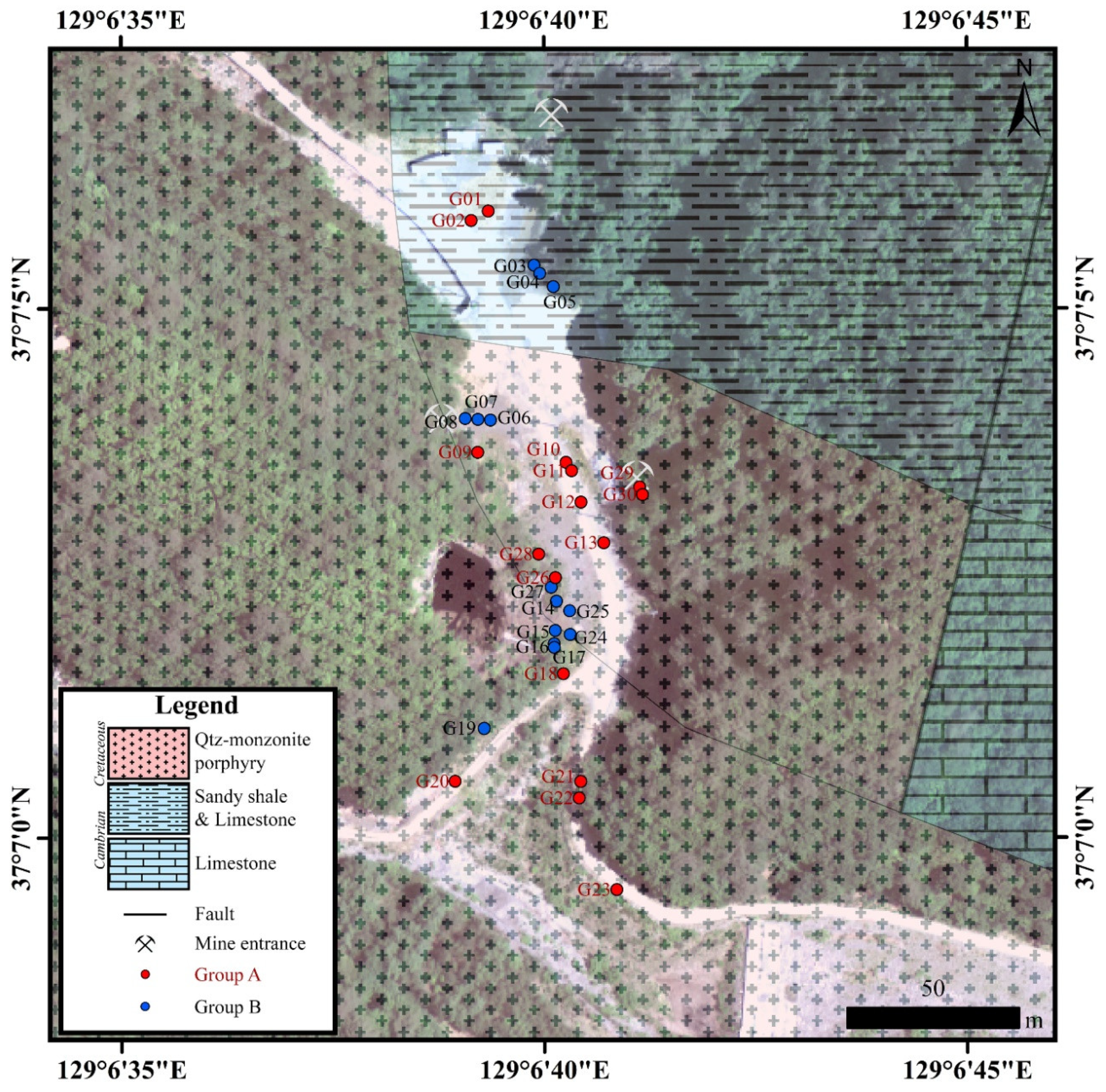
2.1. Study Area
2.2. Sample Collection and Preparation
2.3. Mineralogical and Chemical Analysis
2.4. Spectral Analysis
2.5. Model Development and Evaluation
3. Results and Discussion
3.1. Mineral Composition and Heavy Metal Concentration
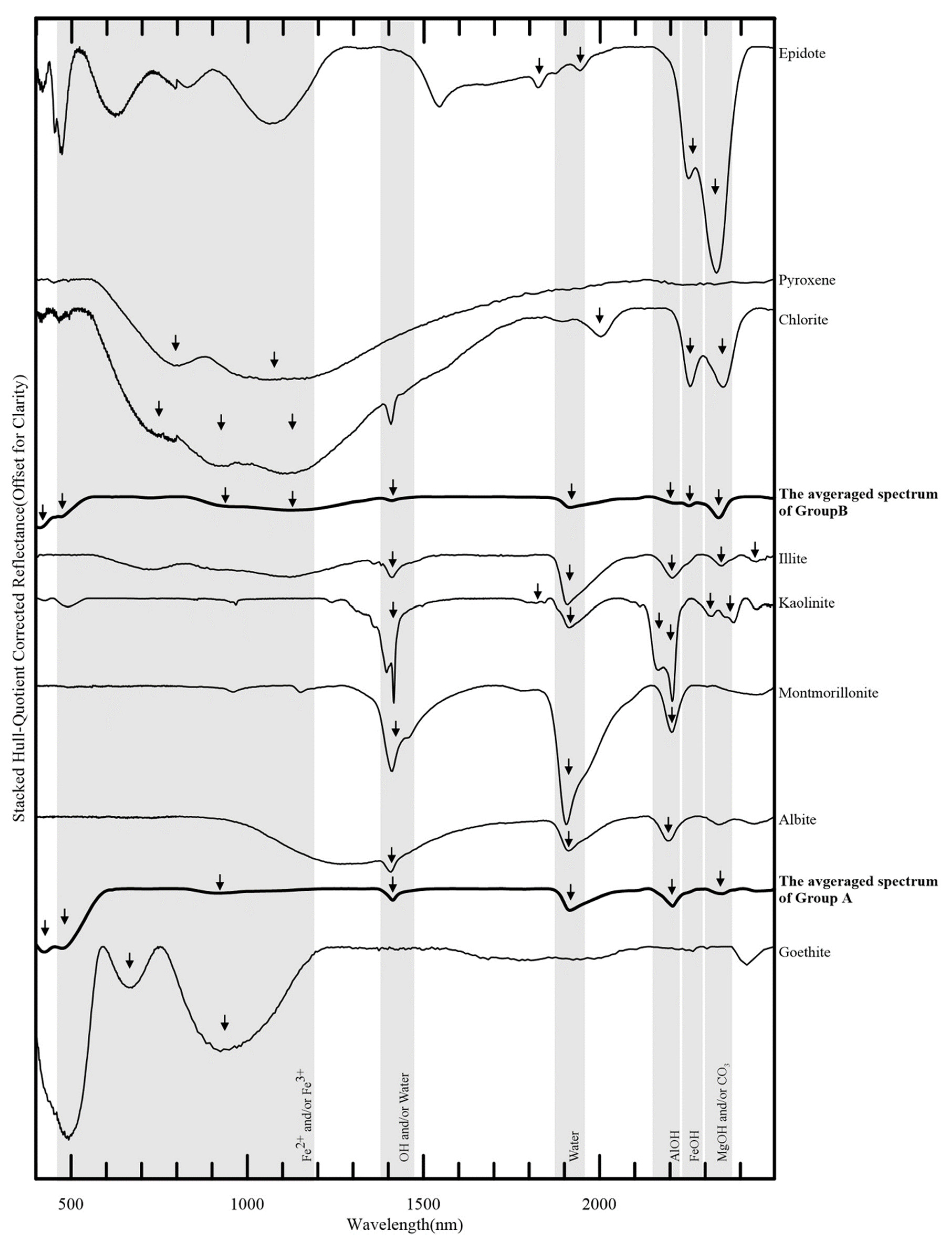
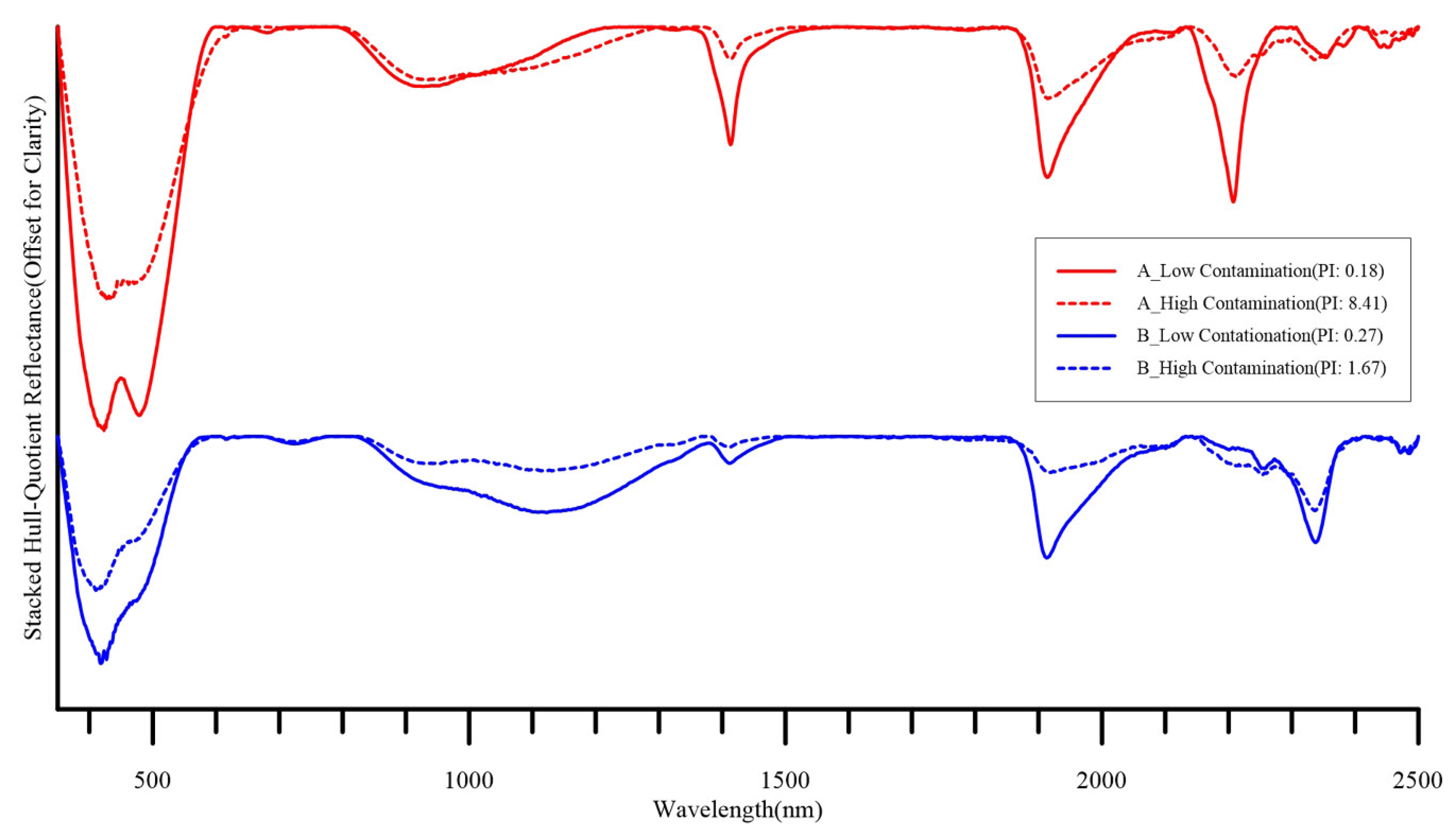
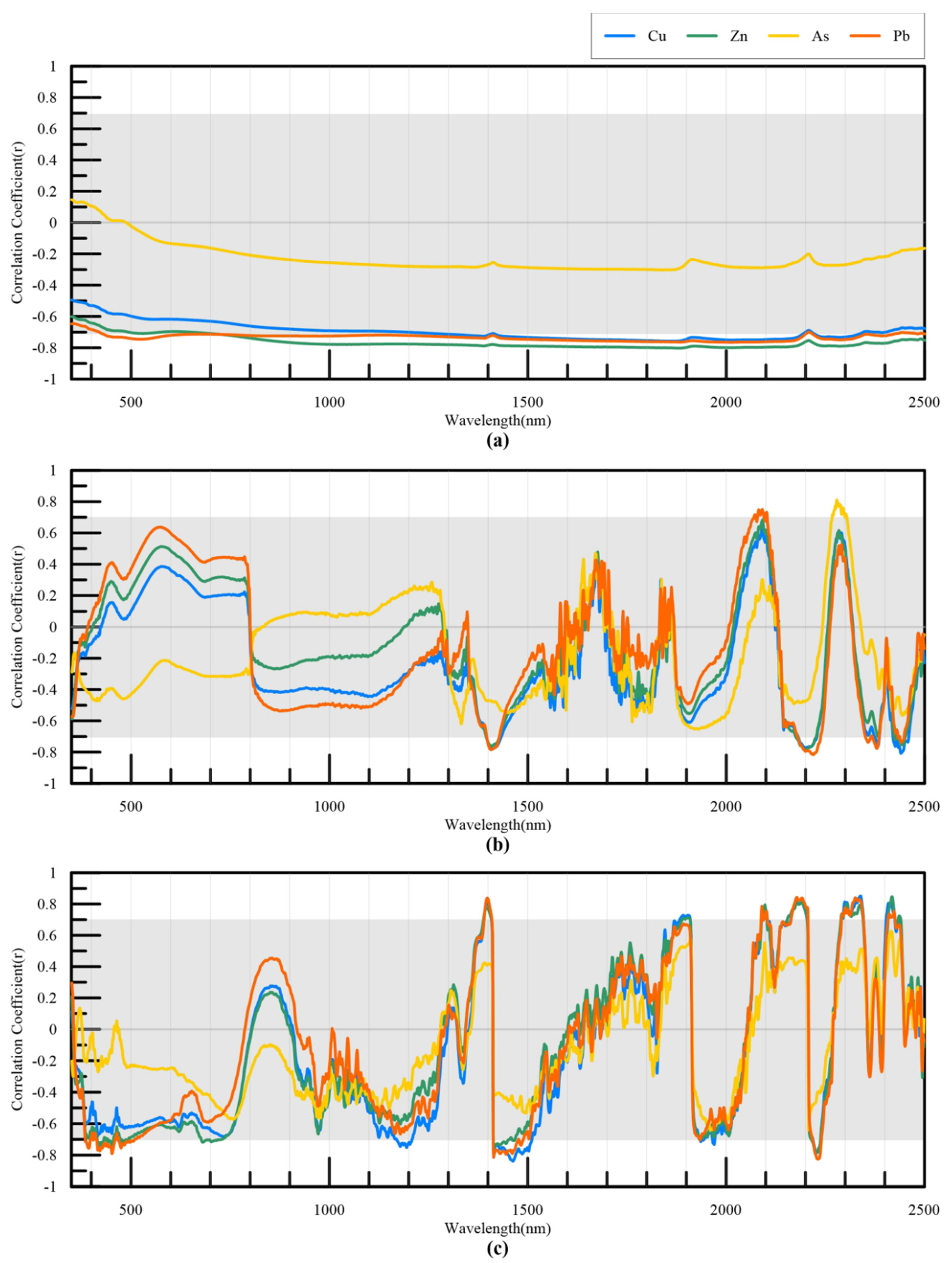
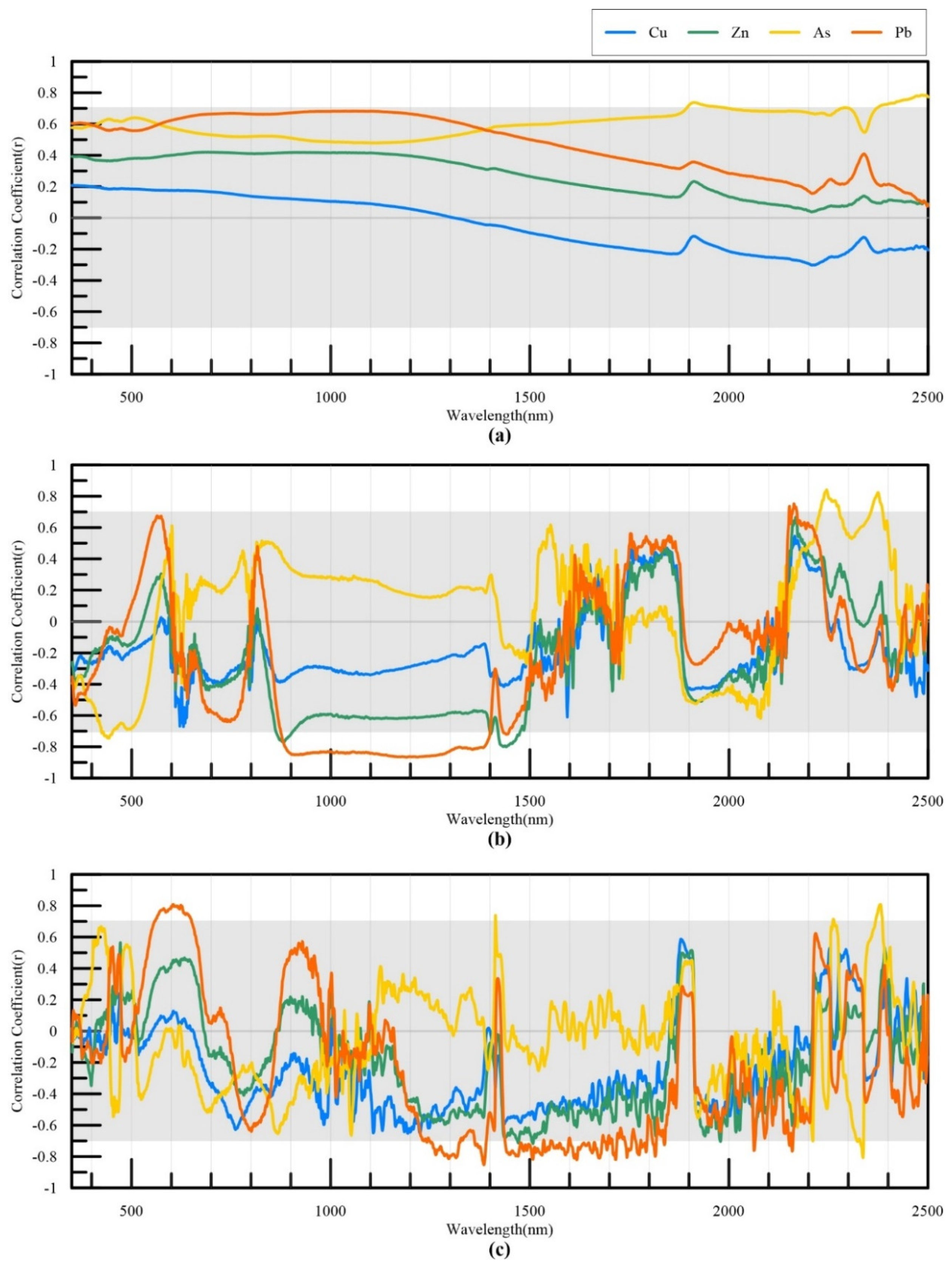
3.2. Spectral Characteristics
3.3. Model Development
3.3.1. Band Selection
3.3.2. Regression Model Development
3.3.3. Regression Model Evaluation
4. Conclusions
Author Contributions
Funding
Acknowledgments
Conflicts of Interest
References
- Van Breemen, N.; Buurman, P. Soil Formation, 2nd ed.; Kluwer Academic Publishers: Dordrecht, The Netherlands, 2002. [Google Scholar]
- Duchaufour, P. Pedology. In Pedogenesis and Classification, 1st ed.; George Allen & Unwin: London, UK, 1982. [Google Scholar]
- Nagajyoti, P.C.; Lee, K.D.; Sreekanth, T.V.M. Heavy metals, occurrence and toxicity for plants: A review. Environ. Chem. Lett. 2010, 8, 199–216. [Google Scholar] [CrossRef]
- Lim, J.; Yu, J.; Wang, L.; Jeong, Y.; Shin, J.H. Heavy Metal Contamination Index Using Spectral Variables for White Precipitates Induced by Acid Mine Drainage: A Case Study of Soro Creek, South Korea. IEEE Trans. Geosci. Remote Sens. 2019, 57, 4870–4888. [Google Scholar] [CrossRef]
- Jeong, Y.; Yu, J.; Wang, L.; Shin, J.H. Spectral Responses of As and Pb Contamination in Tailings of a Hydrothermal Ore Deposit: A Case Study of Samgwang Mine, South Korea. Remote Sens. 2018, 10, 1830. [Google Scholar] [CrossRef] [Green Version]
- Nriagu, J.O. A Global Assesment of Natural Sources of Atmospheric Trace Metals. Nature 1989, 338, 47–49. [Google Scholar] [CrossRef]
- Environmental Protection Agency. Soil Screening Guidance: User’s Guide; U.S. Environmental Protection Agency: Washington, DC, USA, 1996. Available online: https://www.epa.gov/superfund/superfund-soil-screening-guidance (accessed on 3 July 2020).
- Soil Environment Conservation Act. Act no.15658 Ministry of Environment of Korea: Sejong City, South Korea. 2018. Available online: http://www.law.go.kr/LSW/eng/engLsSc.do?menuId=2§ion =lawNm&query=soil&x=0&y=0#liBgcolor15 (accessed on 3 July 2020).
- Von Steiger, B.; Webster, R.; Schulin, R.; Lehmann, R. Mapping heavy metals in polluted soil by disjunctive kriging. Environ. Pollut. 1996, 94, 205–215. [Google Scholar] [CrossRef]
- Shi, T.; Chen, Y.; Liu, Y.; Wu, G. Visible and near-infrared reflectance spectroscopy—An alternative for monitoring soil contamination by heavy metals. J. Hazard. Mater. 2014, 265, 166–176. [Google Scholar] [CrossRef]
- Rathod, P.H.; Rossiter, D.G.; Noomen, M.F.; Van Der Meer, F.D. Proximal Spectral Sensing to Monitor Phytoremediation of Metal-Contaminated Soils. Int. J. Phytoremediation 2013, 15, 405–426. [Google Scholar] [CrossRef]
- Rossel, R.A.V.; Walvoort, D.; McBratney, A.; Janik, L.; Skjemstad, J. Visible, near infrared, mid infrared or combined diffuse reflectance spectroscopy for simultaneous assessment of various soil properties. Geoderma 2006, 131, 59–75. [Google Scholar] [CrossRef]
- Choe, E.; Van Der Meer, F.; Van Ruitenbeek, F.; Van Der Werff, H.; De Smeth, B.; Kim, K.-W. Mapping of heavy metal pollution in stream sediments using combined geochemistry, field spectroscopy, and hyperspectral remote sensing: A case study of the Rodalquilar mining area, SE Spain. Remote Sens. Environ. 2008, 112, 3222–3233. [Google Scholar] [CrossRef]
- Song, L.; Jian, J.; Tan, D.-J.; Xie, H.-B.; Luo, Z.-F.; Gao, B. Estimate of heavy metals in soil and streams using combined geochemistry and field spectroscopy in Wan-sheng mining area, Chongqing, China. Int. J. Appl. Earth Obs. Geoinf. 2015, 34, 1–9. [Google Scholar] [CrossRef]
- Vega, F.; Covelo, E.; Andrade, M.L. Competitive sorption and desorption of heavy metals in mine soils: Influence of mine soil characteristics. J. Colloid Interface Sci. 2006, 298, 582–592. [Google Scholar] [CrossRef] [PubMed]
- Brian, J.A. Heavy Metals in Soils, 3rd ed.; Springer: Dordrecht, The Netherlands, 2013. [Google Scholar]
- Rossel, R.A.V.; Behrens, T. Using data mining to model and interpret soil diffuse reflectance spectra. Geoderma 2010, 158, 46–54. [Google Scholar] [CrossRef]
- Wang, F.; Gao, J.; Zha, Y. Hyperspectral sensing of heavy metals in soil and vegetation: Feasibility and challenges. ISPRS J. Photogramm. Remote Sens. 2018, 136, 73–84. [Google Scholar] [CrossRef]
- Kemper, T.; Sommer, S. Estimate of Heavy Metal Contamination in Soils after a Mining Accident Using Reflectance Spectroscopy. Environ. Sci. Technol. 2002, 36, 2742–2747. [Google Scholar] [CrossRef] [PubMed]
- Al Maliki, A.; Bruce, D.; Owens, G. Prediction of lead concentration in soil using reflectance spectroscopy. Environ. Technol. Innov. 2014, 1, 8–15. [Google Scholar] [CrossRef]
- Shin, J.H.; Yu, J.; Wang, L.; Kim, J.; Koh, S.-M.; Kim, S.-O. Spectral Responses of Heavy Metal Contaminated Soils in the Vicinity of a Hydrothermal Ore Deposit: A Case Study of Boksu Mine, South Korea. IEEE Trans. Geosci. Remote Sens. 2019, 57, 4092–4106. [Google Scholar] [CrossRef]
- Shin, H.; Yu, J.; Wang, L.; Jeong, Y.; Kim, J. Spectral Interference of Heavy Metal Contamination on Spectral Signals of Moisture Content for Heavy Metal Contaminated Soils. IEEE Trans. Geosci. Remote Sens. 2020, 58, 2266–2275. [Google Scholar] [CrossRef]
- Yun, S.; Einaudi, M.T. Zinc-lead skarns of the Yeonhwa-Ulchin District, South Korea. Econ. Geol. 1982, 77, 1013–1032. [Google Scholar] [CrossRef]
- Geological Society of Korea. Geology of Korea; Sigmapress: Seoul, Korea, 1999. [Google Scholar]
- Choi, B.-K.; Choi, S.-G.; Seo, J.; Yoo, I.-K.; Kang, H.-S.; Koo, M.-H. Mineralogical and Geochemical Characteristics of the Wolgok-Seongok Orebodies in the Gagok Skarn Deposit: Their Genetic Implications. J. Econ. Environ. Geol. 2010, 43, 477–490. Available online: https://www.koreascience.or.kr/article/JAKO201012259055703.page (accessed on 3 July 2020).
- Kim, J.D. Assessment of Pollution Level and Contamination Status on Mine Tailings and Soil in the Vicinity of Disused Metal Mines in Kangwon Province. J. Korean Soc. Environ. Eng. 2005, 27, 626–634. Available online: https://www.koreascience.or.kr/article/JAKO200509905714581.page (accessed on 3 July 2020).
- Lee, P.-K.; Kang, M.-J.; Choi, S.-H. Temporal and Spatial Variation and Removal Efficiency of Heavy Metals in the Stream Water Affected by Leachate from the Jiknaegol Tailings Impoundment of the Yeonhwa II Mine. J. Soil Groundw. Environ. 2011, 16, 19–31. [Google Scholar] [CrossRef] [Green Version]
- U.S. EPA. Method 6200: Field Portable X-Ray Fluorescence Spectrometry for the Determination of Elemental Concentrations in Soil and Sediment. 2007. Available online: https://www.epa.gov/hw-sw846/sw-846-test-method-6200-field-portable-x-ray-fluorescence-spectrometry-determination (accessed on 3 July 2020).
- National Institute Occupational Safety Health (NIOSH). Method 7702: Lead by Field Portable XRF; Cincinnati, OH, USA, 1998. Available online: https://www.cdc.gov/niosh/docs/2003-154/pdfs/7702.pdf (accessed on 5 September 2020).
- Zhu, Y.; Weindorf, D.C.; Zhang, W. Characterizing soils using a portable X-ray fluorescence spectrometer: 1. Soil texture. Geoderma 2011, 167–177. [Google Scholar] [CrossRef]
- Lawryk, N.J.; Feng, H.A.; Chen, B.T. Laboratory Evaluation of a Field-Portable Sealed Source X-Ray Fluorescence Spectrometer for Determination of Metals in Air Filter Samples. J. Occup. Environ. Hyg. 2009, 6, 433–445. [Google Scholar] [CrossRef] [PubMed]
- Weindorf, D.C.; Zhu, Y.; McDaniel, P.; Valerio, M.; Lynn, L.; Michaelson, G.; Clark, M.; Ping, C.L. Characterizing soils via portable x-ray fluorescence spectrometer: 2. Spodic and Albic horizons. Geoderma 2012, 189–190, 268–277. [Google Scholar] [CrossRef]
- Weindorf, D.C.; Zhu, Y.; Chakraborty, S.; Bakr, N.; Huang, B. Use of portable X-ray fluorescence spectrometry for environmental quality assessment of peri-urban agriculture. Environ. Monit. Assess. 2011, 184, 217–227. [Google Scholar] [CrossRef]
- Sparks, D.L. Environmetal Soil Chemistry, 1st ed.; Academic Press: San Diego, CA, USA, 1995. [Google Scholar]
- Weindorf, D.C.; Paulette, L.; Man, T. In-situ assessment of metal contamination via portable X-ray fluorescence spectroscopy: Zlatna, Romania. Environ. Pollut. 2013, 182, 92–100. [Google Scholar] [CrossRef]
- Carr, R.; Zhang, C.; Moles, N.; Harder, M. Identification and mapping of heavy metal pollution in soils of a sports ground in Galway City, Ireland, using a portable XRF analyser and GIS. Environ. Geochem. Health 2007, 30, 45–52. [Google Scholar] [CrossRef]
- Sacristán, D.; Rossel, R.V.; Recatalá, L. Proximal sensing of Cu in soil and lettuce using portable X-ray fluorescence spectrometry. Geoderma 2016, 265, 6–11. [Google Scholar] [CrossRef]
- Savitzky, A.; Golay, M.J.E. Smoothing and Differentiation of Data by Simplified Least Squares Procedures. Anal. Chem. 1964, 36, 1627–1639. [Google Scholar] [CrossRef]
- Kokaly, R. Spectroscopic Determination of Leaf Biochemistry Using Band-Depth Analysis of Absorption Features and Stepwise Multiple Linear Regression. Remote Sens. Environ. 1999, 67, 267–287. [Google Scholar] [CrossRef]
- Clark, R.N.; Swayze, G.A.; Wise, R.A.; Livo, K.E.; Hoefen, T.M.; Kokaly, R.F.; Sutley, S.J. USGS Digital Spectral Library splib06a. In Data Series 231; US Geological Survey: Reston, VA, USA, 2007. [Google Scholar] [CrossRef]
- Kokaly, R.F.; Clark, R.N.; Swayze, G.A.; Livo, K.E.; Hoefen, T.M.; Pearson, N.C.; Wise, R.A.; Benzel, W.M.; Lowers, H.A.; Driscoll, R.L.; et al. USGS Spectral Library Version 7. Data Ser. 1035 2017. [Google Scholar] [CrossRef]
- Baldridge, A.M.; Hook, S.; Grove, C.; Rivera, G. The ASTER spectral library version 2.0. Remote Sens. Environ. 2009, 113, 711–715. [Google Scholar] [CrossRef]
- Vasques, G.; Grunwald, S.; Sickman, J. Comparison of multivariate methods for inferential modeling of soil carbon using visible/near-infrared spectra. Geoderma 2008, 146, 14–25. [Google Scholar] [CrossRef]
- Dunagan, S.C.; Gilmore, M.S.; Varekamp, J. Effects of mercury on visible/near-infrared reflectance spectra of mustard spinach plants (Brassica rapa P.). Environ. Pollut. 2007, 148, 301–311. [Google Scholar] [CrossRef] [PubMed]
- Shin, H.; Yu, J.; Jeong, Y.; Wang, L.; Yang, D.-Y. Case-Based Regression Models Defining the Relationships Between Moisture Content and Shortwave Infrared Reflectance of Beach Sands. IEEE J. Sel. Top. Appl. Earth Obs. Remote Sens. 2017, 10, 4512–4521. [Google Scholar] [CrossRef]
- Williams, P.; Norris, K. Near-Infrared Technology in the Agricultural and Food Industries; American Association of Cereal Chemists, Inc.: St. Paul, MN, USA, 1987. [Google Scholar]
- Chang, C.-W.; Laird, D.A.; Mausbach, M.J.; Hurburgh, C.R. Near-Infrared Reflectance Spectroscopy-Principal Components Regression Analyses of Soil Properties. Soil Sci. Soc. Am. J. 2001, 65, 480–490. [Google Scholar] [CrossRef] [Green Version]
- Wu, Y.Z.; Chen, J.; Ji, J.F.; Tian, Q.J.; Wu, X.M. Feasibility of Reflectance Spectroscopy for the Assessment of Soil Mercury Contamination. Environ. Sci. Technol. 2005, 39, 873–878. [Google Scholar] [CrossRef]
- Sipos, P.; Németh, T.; Kis, V.K.; Mohai, I. Sorption of copper, zinc and lead on soil mineral phases. Chemosphere 2008, 73, 461–469. [Google Scholar] [CrossRef]
- Madrid, L.; Diaz-Barrientos, E. Influence of carbonate on the reaction of heavy metals in soils. J. Soil Sci. 1992, 43, 709–721. [Google Scholar] [CrossRef]
- Kim, S.-O.; Lee, W.C.; Jeong, H.-S.; Cho, H.G. Adsorption of Arsenic on Goethite. J. Mineral. Soc. Korea 2009, 22, 177–189. Available online: https://www.koreascience.or.kr/article/JAKO200908856864167.page (accessed on 3 July 2020).
- Kim, S.H.; Lee, W.C.; Cho, H.G.; Kim, S.-O. Characterization of Arsenic Adsorption onto Hematite. J. Miner. Soc. Korea 2012, 25, 197–210. [Google Scholar] [CrossRef]
- Pontual, S.; Gamsom, P.; Merry, N. Spectral Interpretation Field Manual: Spectral Analysis Guides for Mineral. Exploration, 1st ed.; AusSpec Int.: Boulder, CO, USA, 2012. [Google Scholar]


| Site No. | Primary Minerals | Accessory Minerals | Group |
|---|---|---|---|
| G01 | Quartz, Plagioclase | Illite, Kaolinite, Biotite, Montmorillonite | A |
| G03 | Calcite, Quartz, Pyroxene | Epidote, Kaolinite | B |
| G04 | Calcite, Quartz | Illite, Chlorite, Kaolinite | B |
| G05 | Calcite, Quartz, Epidote | Pyroxene | B |
| G08 | Quartz, Pyroxene, Calcite | Epidote, Kaolinite, Montmorillonite | B |
| G09 | Quartz, Plagioclase, Illite | Kaolinite | A |
| G11 | Quartz, Plagioclase | Kaolinite, Montmorillonite | A |
| G12 | Quartz, Plagioclase | Kaolinite, Montmorillonite | A |
| G14 | Epidote, Pyroxene, Quartz | Calcite, Kaolinite, Illite | B |
| G15 | Epidote, Chlorite | Quartz | B |
| G16 | Calcite, Pyroxene | - | B |
| G18 | Plagioclase, Quartz, K-Feldspar | Illite, Calcite | A |
| G19 | Calcite | Plagioclase, Quartz, Kaolinite | B |
| G20 | Quartz, Plagioclase | Kaolinite, Phlogopite | A |
| G22 | Quartz, Plagioclase | Chlorite, Kaolinite, Biotite | A |
| G23 | Plagioclase, Quartz, Illite | Kaolinite, Biotite | A |
| G25 | Pyroxene, Epidote | Quartz | B |
| G30 | Quartz, Plagioclase | Illite, Calcite | A |
| Element | Group A (n = 99) | Group B (n = 84) | Soil Pollution Standard | ||||||
|---|---|---|---|---|---|---|---|---|---|
| Statistics | Statistics | ||||||||
| Min | Max | Mean | SD | Min | Max | Mean | SD | ||
| Cu | 0 | 363 | 144 | 124 | 0 | 172 | 106 | 41 | 500 |
| Zn | 82 | 15,167 | 5477 | 4466 | 143 | 3014 | 1004 | 682 | 600 |
| As | 0 | 349 | 95 | 91 | 27 | 116 | 63 | 63 | 50 |
| Pb | 27 | 1268 | 541 | 375 | 30 | 327 | 103 | 79 | 400 |
| Group A | (n = 99) | Group B | (n = 84) | ||||||
|---|---|---|---|---|---|---|---|---|---|
| Cu | Zn | As | Pb | Cu | Zn | As | Pb | ||
| Cu | 1.00 | Cu | 1.00 | ||||||
| Zn | 0.84 | 1.00 | Zn | 0.41 | 1.00 | ||||
| As | 0.55 | 0.57 | 1.00 | As | 0.06 | 0.05 | 1.00 | ||
| Pb | 0.85 | 0.85 | 0.26 | 1.00 | Pb | 0.33 | 0.86 | 0.01 | 1.00 |
| Elements | Wavelength | β0 | β1 (SE) | β2 (SE) | β3 (SE) | F | R2 | Adj-R2 | RMSE (mg·kg−1) | NRMSE (%) |
|---|---|---|---|---|---|---|---|---|---|---|
| Reflectance | ||||||||||
| Zn | 1884 nm | 27,932 | −37,907 (3619) *** | 109.7 | 0.621 | 2880 | 19.1 | |||
| Absorption depth | ||||||||||
| Cu | 2442 nm, 2383 nm | 318 | −13,099 (2649) *** | −10,422 (3808) *** | 77.1 | 0.691 | 68 | 18.8 | ||
| Zn | 2441 nm, 2200 nm | 13,199 | −405,254 (149,575) ** | −75,832 (29,849) * | 56.0 | 0.618 | 2870 | 19.0 | ||
| As | 2279 nm | −26 | 26,251 (2225) *** | 139.1 | 0.675 | 54 | 15.3 | |||
| Pb | 2220 nm, 2356 nm | 1305 | −11,913 (2441) *** | −16,582 (5591) *** | 70.0 | 0.67 | 220 | 17.7 | ||
| First derivatives | ||||||||||
| Cu | 2337 nm, 1510 nm, 2410 nm | 488 | 217,583 (41,479) *** | −1,165,632 (283,556) *** | 224,261 (66,445) *** | 110.9 | 0.829 | 51 | 14.0 | |
| Zn | 2419 nm, 1890 nm, 2410 nm | 15,756 | 30,762,496 (2,912,237) *** | −7,779,064 (1,273,252) *** | 13,646,303 (3,329,708) *** | 112.7 | 0.831 | 1907 | 12.6 | |
| Pb | 2178 nm, 2220 nm | 1356 | 1,549,406 (188,336) *** | 373,484 (91,923) *** | 101.9 | 0.748 | 193 | 15.5 | ||
| Elements | Wavelength | β0 | β1 (SE) | β2 (SE) | F | R2 | Adj-R2 | RMSE (mg·kg−1) | NRMSE (%) |
|---|---|---|---|---|---|---|---|---|---|
| Absorption Depth | |||||||||
| Zn | 1440 nm | 2477 | −2,228,796 (23,681) *** | 93.4 | 0.621 | 434 | 15.1 | ||
| Pb | 1190 nm | 292 | −4321 (265) *** | 140.4 | 0.711 | 42 | 14.2 | ||
| First Derivatives | |||||||||
| Pb | 1773 nm, 2065 nm | 279 | −1,422,971 (181,834) *** | −968,853 (156,127) *** | 131.0 | 0.818 | 33 | 11.2 | |
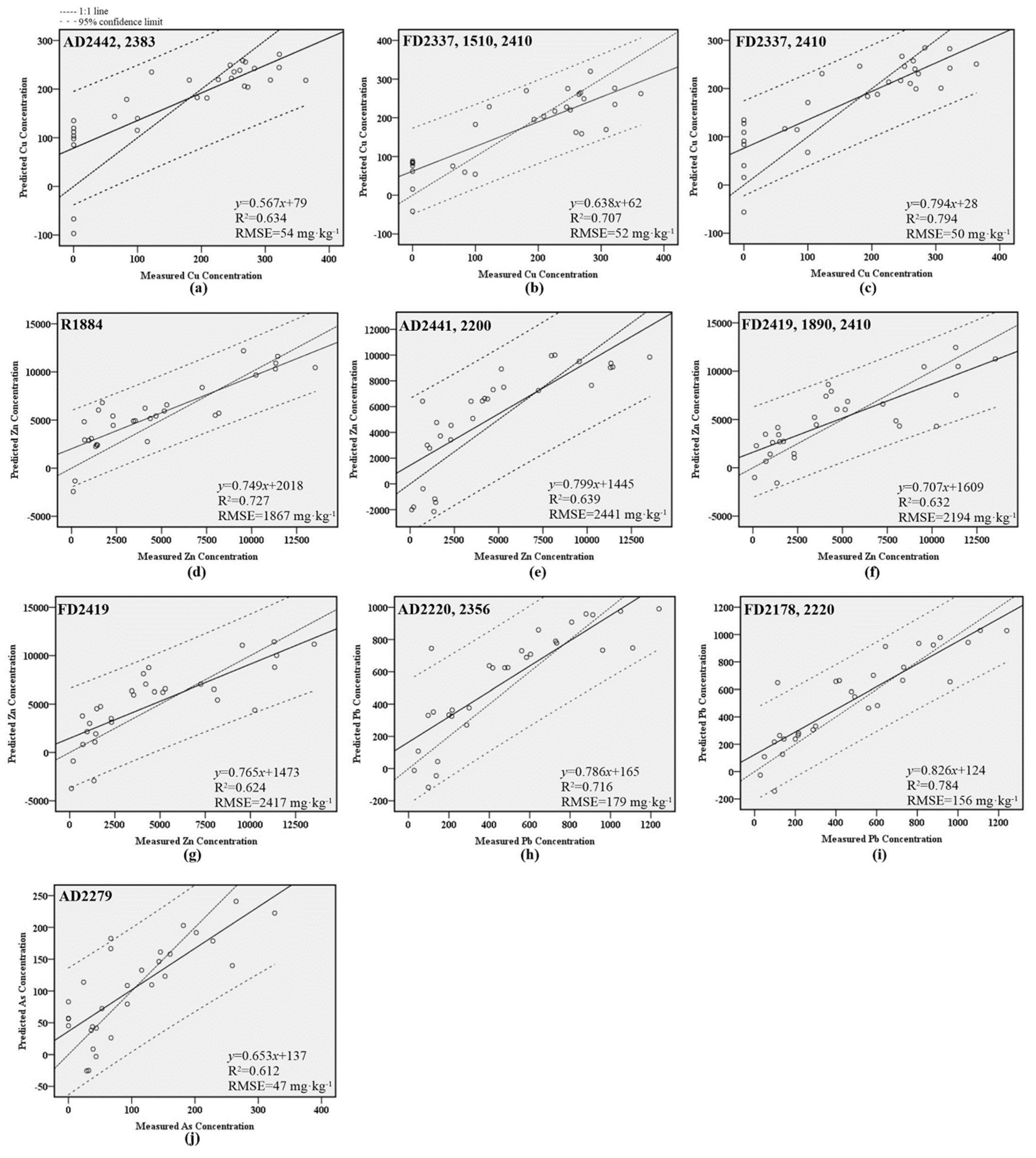
| Element | Wavelength Selection | a | b | R2 | RMSE (mg·kg−1) | NRMSE (%) | RPD |
|---|---|---|---|---|---|---|---|
| Reflectance | |||||||
| Zn | 1884 nm | 0.749 | 2018 | 0.727 | 1867 | 12.4 | 1.88 |
| Absorption Depth | |||||||
| Cu | 2442 nm, 2383 nm | 0.567 | 79 | 0.634 | 54 | 15.0 | 1.62 |
| Zn | 2441 nm, 2200 nm | 0.799 | 1445 | 0.639 | 2441 | 16.2 | 1.64 |
| As | 2279 nm | 0.653 | 37 | 0.612 | 47 | 13.4 | 1.58 |
| Pb | 2220 nm, 2356 nm | 0.786 | 165 | 0.716 | 179 | 14.4 | 1.84 |
| First Derivatives | |||||||
| Cu | 2337 nm, 1510 nm, 2410 nm | 0.638 | 62 | 0.707 | 52 | 14.3 | 1.82 |
| 2337 nm, 2410 nm | 0.794 | 28 | 0.794 | 50 | 13.8 | 1.72 | |
| Zn | 2419 nm, 1890 nm, 2410 nm | 0.707 | 1609 | 0.632 | 2194 | 14.5 | 1.62 |
| 2419 nm | 0.765 | 1473 | 0.624 | 2417 | 16.0 | 1.60 | |
| Pb | 2178 nm, 2220 nm | 0.826 | 124 | 0.784 | 156 | 12.6 | 2.12 |
| Element | Wavelength Selection | a | b | R2 | RMSE (mg·kg−1) | NRMSE (%) | RPD |
|---|---|---|---|---|---|---|---|
| Absorption Depth | |||||||
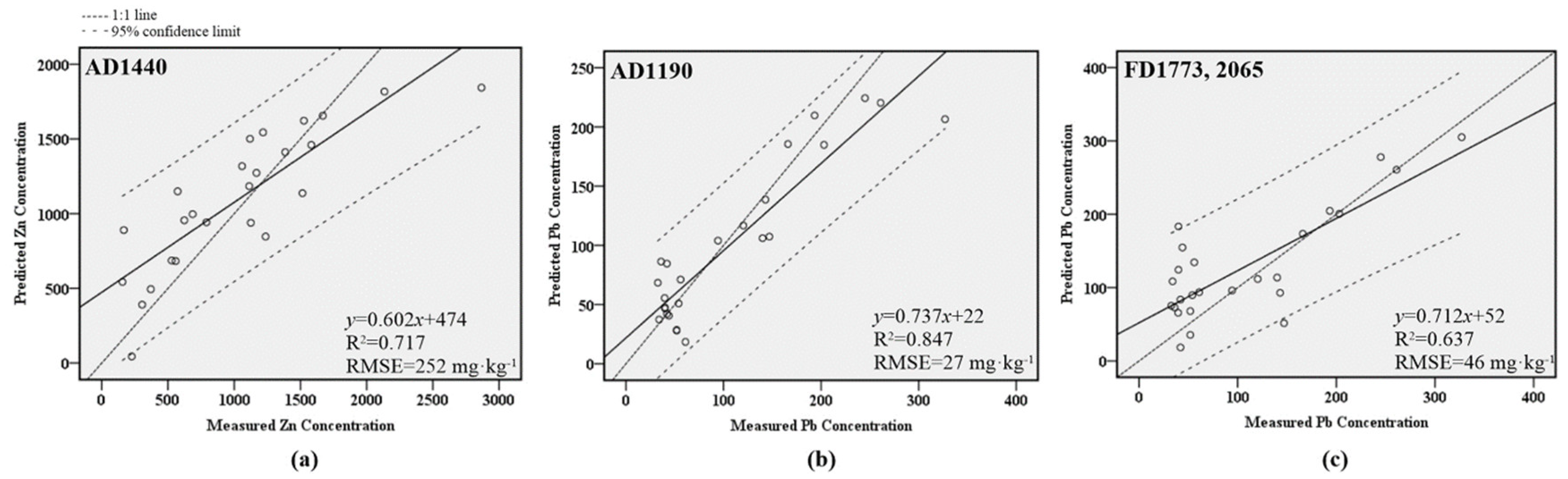
| Zn | 1440 nm | 0.602 | 474 | 0.717 | 252 | 8.8 | 1.84 |
| Pb | 1190 nm | 0.737 | 22 | 0.847 | 27 | 9.1 | 2.50 |
| First Derivatives | |||||||
| Pb | 1773 nm, 2065 nm | 0.712 | 52 | 0.637 | 46 | 15.6 | 1.63 |
© 2020 by the authors. Licensee MDPI, Basel, Switzerland. This article is an open access article distributed under the terms and conditions of the Creative Commons Attribution (CC BY) license (http://creativecommons.org/licenses/by/4.0/).
Share and Cite
Kim, H.; Yu, J.; Wang, L.; Jeong, Y.; Kim, J. Variations in Spectral Signals of Heavy Metal Contamination in Mine Soils Controlled by Mineral Assemblages. Remote Sens. 2020, 12, 3273. https://doi.org/10.3390/rs12203273
Kim H, Yu J, Wang L, Jeong Y, Kim J. Variations in Spectral Signals of Heavy Metal Contamination in Mine Soils Controlled by Mineral Assemblages. Remote Sensing. 2020; 12(20):3273. https://doi.org/10.3390/rs12203273
Chicago/Turabian StyleKim, Hyesu, Jaehyung Yu, Lei Wang, Yongsik Jeong, and Jieun Kim. 2020. "Variations in Spectral Signals of Heavy Metal Contamination in Mine Soils Controlled by Mineral Assemblages" Remote Sensing 12, no. 20: 3273. https://doi.org/10.3390/rs12203273