Deriving Annual Double-Season Cropland Phenology Using Landsat Imagery

Abstract

Cropland phenology provides key information in managing agricultural practices and modelling crop yield. However, most of the existing phenological products have coarse spatial resolution ranging from 250 to 8000 m, which is not sufficient to capture the critical spatial details of cropland phenology at the landscape scale. Landsat imagery provides an unprecedented data source to generate 30-m spatial resolution phenological products. This paper explored the potential of utilizing multi-year Landsat enhanced vegetation index to derive annual phenological metrics of a double-season agricultural land from 1993 to 2009 in a sub-urban area of Shanghai, China. We used all available Landsat TM and ETM+ observations (538 scenes) and developed a Landsat double-cropping phenology (LDCP) algorithm. LDCP captures the temporal trajectory of multi-year enhanced vegetation index time series very well, with the degree of fitness ranging from 0.78 to 0.88 over the study regions. We found good agreements between derived annual phenological metrics and in situ observation, with root mean square error ranging from 8.74 to 18.04 days, indicating that the proposed LDCP is capable of detecting double-season cropland phenology. LDCP could reveal the spatial heterogeneity of cropland phenology at parcel scales. Phenology metrics were retrieved for approximately one-third and two-thirds of the 17 years for the first and second cropping cycles, respectively, depending on the number of good quality Landsat data. In addition, we found an advanced peak of season for both cropping cycles in 50–60% of the study area, and a delayed start of season for the second cropping cycle in 50–70% of the same area. The potential drivers of those trends might be climate warming and changes in agricultural practices. The derived cropland phenology can be used to help estimate historical crop yields at Landsat spatial resolution, providing insights on evaluating the effects of climate change on temporal variations of crop growth, and contributing to food security policy making.

1. Introduction

Cropland serves as the foundation of the stability of the society, producing foods and many other goods that are vital to human wellbeing [1]. Agricultural practices such as irrigation, fertilization, and crop rotation, also affect energy, water, and carbon cycles between land and atmosphere [2]. Phenological stages of the cropland, i.e., the timing of start and peak of the growing season, can provide key information about agricultural practices [3]. Accurate cropland phenology can help model crop yield, thus contributing towards the understanding of global food security in the 21st century [4,5].

Remote sensing is widely used to estimate cropland phenology, because it provides consistent and frequent observations over large spatial domains. Researchers derived phenological parameters of cropland using time series of spectral vegetation indices obtained from satellite instruments, such as advanced very high resolution radiometer (AVHRR) and moderate resolution imaging spectroradiometer (MODIS). For example, de Beurs and Henebry [6] modelled normalized difference vegetation index (NDVI) from the AVHRR dataset as a quadratic function of accumulated growing degree-days (AGDD) in Kazakhstan. Brown et al. [7] extended this method and estimated the start of the growing season, peak growth timing, and the length of the growing season in regions with rainfed cropland at a global scale. Sakamoto et al. [8] applied a wavelet transformation to a MODIS enhanced vegetation index (EVI) dataset and derived phenological stages of paddy rice in Japan. Sakamoto, Wardlow, Gitelson, Verma, Suyker and Arkebauer [3] also used a ‘shape-model fitting’ procedure to calculate phenological metrics of maize and soybean based on MODIS wide dynamic range vegetation index (WDRVI). In addition, studies have reported that multiple growth periods of cropland can be described by step-wise logistic functions [9,10].

However, the spatial resolution of the existing phenological products is coarse (250–8000 m) for croplands. Unlike natural vegetation such as deciduous and mixed forests, the driving factors of spatial variations in cropland phenology are much more complicated, due to a great variety of agricultural practices from different households (irrigation, fertilization usage, and crop types). Mixed land cover types (e.g., grasslands, forests, rural houses, and roads) inevitably existed within the field view of coarse spatial resolution instruments, thus biasing the estimation of phenological metrics. In comparison, Landsat imagery provides the potential to capture sufficient phenology details at 30-m spatial resolution. However, the revisit time interval provided by a single Landsat sensor is too long, hindering estimates of key phenological events when using only one year of data, particularly in regions with less cloud-free images. To address this limitation, researchers have developed three strategies. The first strategy is to produce Landsat-scale surface reflectance from MODIS imagery by integrating the spatial details from Landsat and temporal information from MODIS [11]. Fused Landsat-MODIS imagery was reported to be capable of detecting green-up dates of corn and soybean in the United States [12]. However, this approach did not allow us to estimate the phenological timing of cropland back at a time when MODIS data does not exist. In addition, land cover heterogeneity within one pixel of MODIS may introduce uncertainties in constructing the Landsat-scale surface reflectance [13], thus reducing the accuracies of the estimated phenological metrics. The data-fusion strategy is more limited in the cropland of China, because cropland parcels that each house owns are usually a small fraction of a hectare [14], i.e., well within one smallest pixel of MODIS (i.e., 6.25 ha). The cropland parcels are also shaped irregularly, following the natural variation of topography and historical boundaries. The variety of crops, the planting, and the irrigation time and the amount of fertilizer used can vary significantly for parcels next to each other. The second strategy is to combine annual Landsat images from different sensors, i.e., Landsat 5 Thematic Mapper (TM) and Landsat 7 Enhanced Thematic Mapper plus (ETM+), thus providing an 8-day revisit time [15]. A recent study has applied linear and non-linear harmonic models to Landsat analysis-ready data and estimated peak NDVI days [15] of major crop types in the conterminous United States (CONUS) in the year 2010. The harmonic models required at least 15 valid observations [15]. This requirement may not be satisfied back in time when Landsat ETM+ was not launched or in regions with persistent cloud cover. The third strategy is to leverage multi-year Landsat images organized by day of year (DOY) to derive long-term mean phenology metrics. This approach has been well demonstrated for deciduous forest [16,17,18,19] and the mixed forest [20], as well as for urban vegetation [21,22]. However, this strategy has not been fully utilized in monitoring annual cropland phenology, particularly for double-season crops, which is one of the most common agricultural systems in southern China. Filling this knowledge gap can provide critical information for understanding climate change impacts on crop development and improving the estimation of crop yields at the Landsat scale. Annual crop phenology metrics can contribute to a better assessment of annual agricultural productivity, and thus contributing to well-informed and effective food security policy making. In this study, we examine the applicability of using Landsat to derive annual phenological stages of double-cropping agricultural land in the rural suburb of Shanghai, China. We pooled all available Landsat 5 TM and Landsat 7 EMT+ from 1993 to 2009 and estimated the start and peak of the season in each year. We provided different metrics to evaluate the effectiveness of the algorithm and the quality of the constructed phenological trajectory. We also validated our results with in situ phenology observations. Finally, we examined the year-to-year variations in phenological metrics and their potential environmental drivers.

2. Materials and Methods

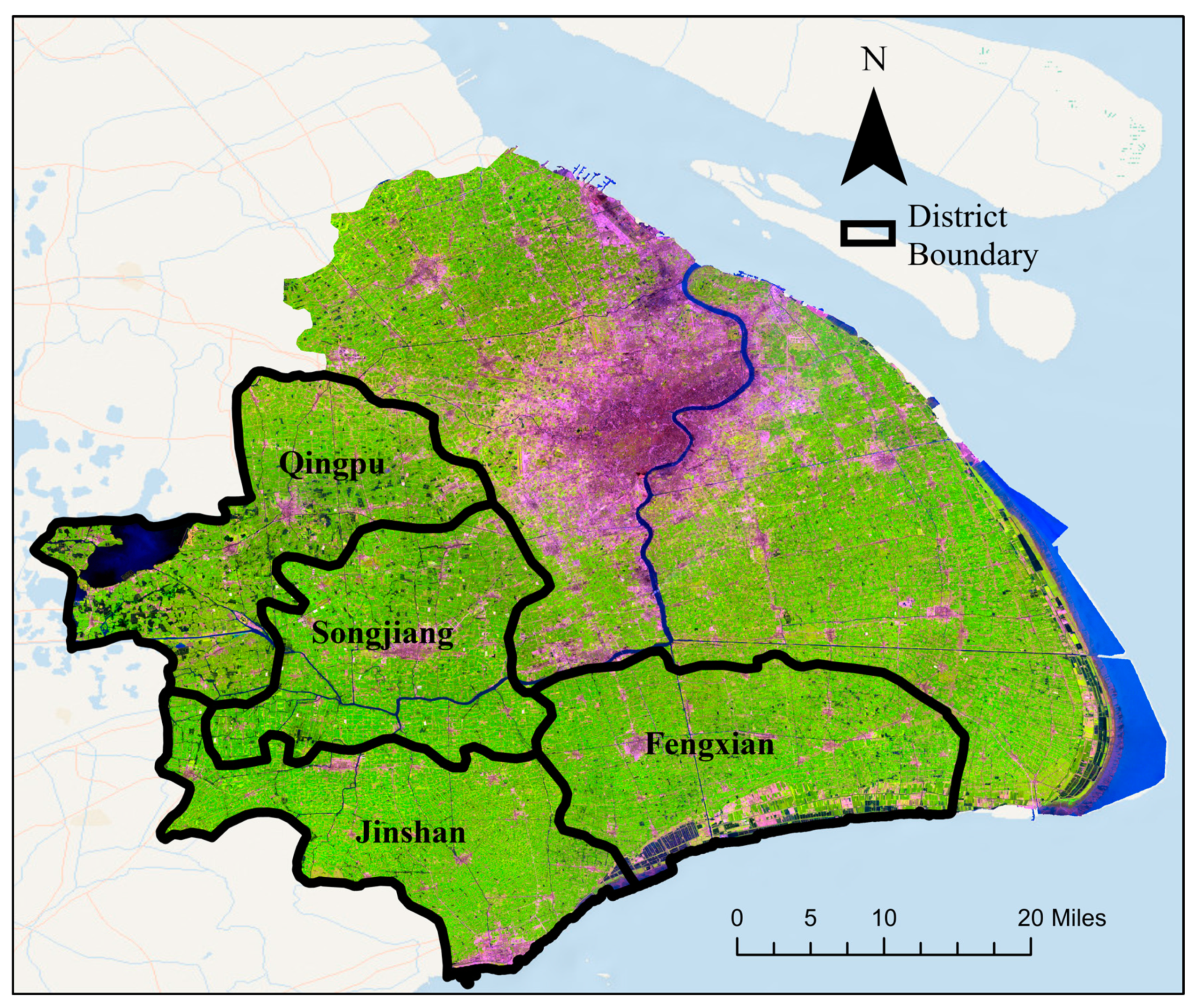
2.1. Study Site and Period

Our study site is located in southwestern Shanghai (Figure 1). Although it is considered the most urbanized city in China, its rural suburbs consist of large regions of fertile croplands, which were protected from development. The subtropical monsoon climate in the region with a mean annual temperature of 17.1 °C and mean annual precipitation of 1166.1 mm is highly suitable for crop cultivation. Croplands in the rural suburbs of Shanghai are intensively managed as a double-cropping system, constituting key food supplies to the city [23,24]. The double cropping system in Shanghai has two types: wheat-rice rotation and rice-rice rotation system. In this study, we specifically focused on four districts, including Jinshan, Fengxian, Qingpu, and Songjiang, because these districts have large areas of double-cropping agricultural land. We choose the study period from 1993 to 2009 based on the availability of the in situ cropland phenology observations, which are critical to validate the model. Note that the proposed approach can be adapted in more recent years when Landsat 8 and Sentinel-2 images are available, but neither sensor was launched in our study period. Landsat 5 and 7 also provided a longer historical time series than Sentinel 2, which are critical to understanding the inter-annual variations of crop growth, and their response to potential climate variations.

2.2. Dataset

We used all available Landsat images from 1993 to 2009 within two scenes (Path 118, Rows 38 and 39), with less than 90% cloud cover. The images come from two sensors, including Landsat 5 TM and Landsat 7 ETM+. We downloaded the surface reflectance data from the United States Geological Survey (https://earthexplorer.usgs.gov/). We then used the F-mask algorithms [25] to remove pixels contaminated by clouds and their shadows. Missing data from the failure of scan line corrector (SLC) in ETM+ were also screened in this study. The final dataset had a total of 538 images. To separate cropland from other land cover/land use (LCLU) types and identify the stable cropland pixels, we utilized the LCLU map in years 1995 and 2010 in Shanghai from a previous study [21]. These LCLU maps included five main land cover types, i.e., water, urban vegetation, cropland, developed land and barren land. The accuracies of cropland in the years 1995 and 2010 were 76% and 80%, respectively. We used the existing LCLU map to remove the pixels that have experienced LCLU changes. Thus, only stable cropland pixels were used in this study.

In situ phenological observations were downloaded from the data center of the Chinese Meteorological Administration (CMA). There is one in situ phenological observation located in our study regions (i.e., Songjiang agro-meteorological station), which may not be sufficient to validate the derived phenological metrics. Therefore, we also obtained in situ data from other cropland stations in two neighboring provinces (i.e., Jiangsu and Anhui) that shared the same double cropping rotation system (wheat-rice rotation) as the Songjiang agro-meteorological station. There are seven agro-meteorological stations in total, including Songjiang, Xinghua, Jianhu, Huaiyin, Xuzhou, Tianchang, and Shouxian (Figure S1). For the first crop season, i.e., winter wheat, the ground observation recorded multiple phenological stages, including the timing of planting, emergence, tillering, jointing, booting, heading, and ripening. For the second crop season, i.e., rice, the ground observation includes the timing of emergence, tillering, booting, heading, and ripening. Missing observations in the ground records were removed in this study. All available clear images (Table S1) from 1993 to 2009 were also downloaded at each of the seven agro-meteorological stations to derive cropland phenology metrics, following the same procedure in our study regions.

2.3. Pre-Process of Landsat Time Series

We first identified stable cropland pixels by excluding pixels that experienced an LCLU change during 1993–2009, using LCLU maps in the years 2010 and 1995 [21]. Enhanced Vegetation Index (EVI) was then calculated from the surface reflectance of all stable cropland pixels using Equation (1).

$$\mathrm{EVI}=2.5\ast \frac{\left({\rho }_{\mathrm{NIR}}-{\rho }_{\mathrm{RED}}\right)}{\left({\rho }_{\mathrm{NIR}}+6.0\times {\rho }_{\mathrm{RED}}-7.5\times {\rho }_{\mathrm{BLUE}}+1.0\right)}$$

(1)

where ${\rho }_{\mathrm{NIR}},{\rho }_{\mathrm{RED}}$ and ${\rho }_{\mathrm{BLUE}}$ are surface reflectance values for the three respective bands. We derived the phenological metrics from EVI because it is more sensitive in densely vegetated regions compared with other vegetation indices [26]. The relatively long revisit time of Landsat satellites, the cloud contamination, and the SLC-off in ETM+ sensor prevent capturing the intra-annual variations of phenology, thus, we stacked all available images from 1993 to 2009 by day of year (DOY), as if they were collected in a single year. To reduce the influence of the inter-annual variations in vegetation greenness magnitude, we normalized the time series using the 10th and 90th percentiles of EVI within each two-year moving window, as described in Melaas et al. [18], leading to a EVI time series with consistent range and amplitude. We referred this normalized time series as normalized EVI (NEVI).

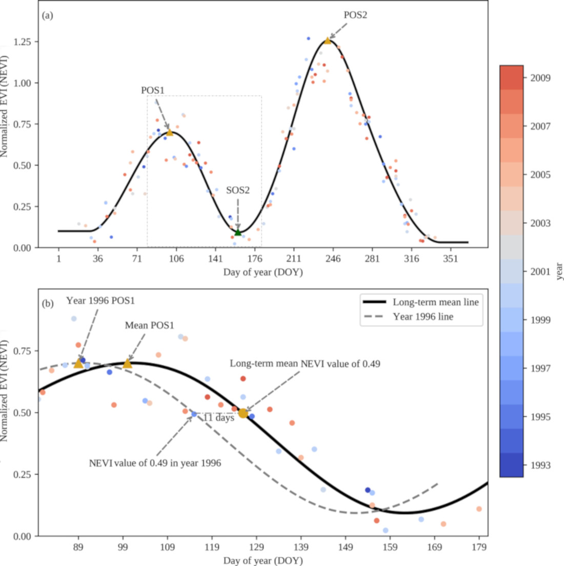
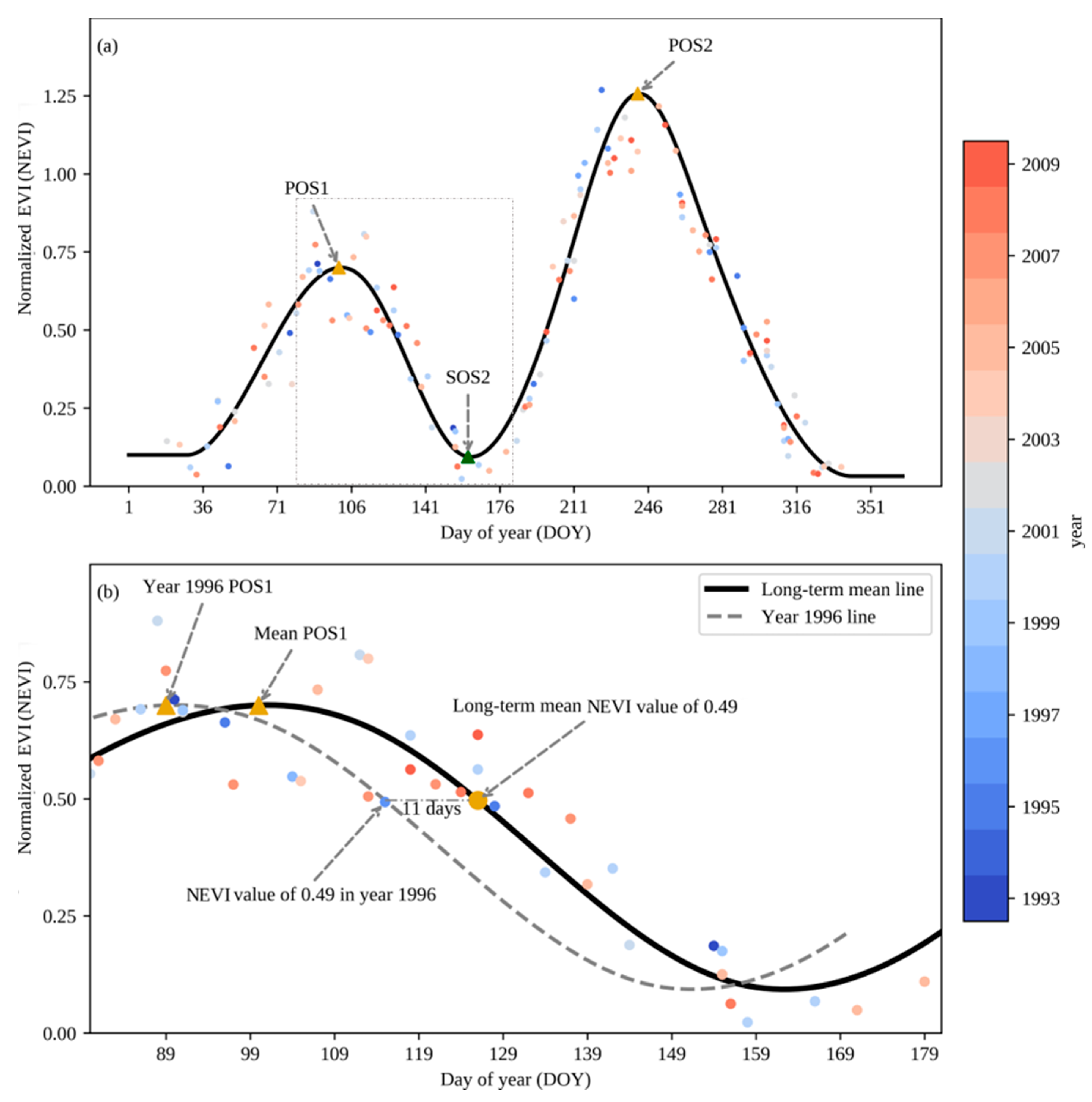
2.4. Detection of Annual Phenological Metrics

In this study, we extended the algorithm proposed by Melaas, Friedl and Zhu [17] and Melaas et al. [18] and developed a Landsat double-cropping phenology (LDCP) to extract annual phenological metrics of double-season cropland. The original method was specifically designed for deciduous and mixed forests. Fewer attempts have been made for double-season croplands, especially for wheat-rice and rice-rice rotation cropping systems. We adapted the algorithm in three major steps. Firstly, a cubic spline model was used to simulate the mean temporal trajectories of normalized EVI (NEVI) at each stable cropland pixel (Figure 2a). Studies have reported that cubic spline could reduce the biases caused by the asymmetric increase or decrease in temporal EVI trajectories of deciduous and mixed forests [18,27]. The cubic spline model is also well-suited for interpolating irregularly spaced data [28], which is the case for stacked multi-year observations from Landsat satellites, due to irregular high quality image acquisition dates. Therefore, it is challenging to apply commonly used filters, such as Savitzky–Golay algorithm [23,29], to smooth Landsat time series. In addition, the cubic spline model is capable of handling missing data and can serve as a robust smoothing tool for the EVI time series [30]. It was also found to be more flexible to identify multiple growth cycles of croplands [30]. The next step is extracting the multi-year average peak of season of the first cropping cycle (POS1), the start of season of the second cropping cycle (SOS2), and the peak of season of the second cropping cycle (POS2). We used an 8-day moving window on the fitted NEVI time series and calculated the slope within each window to identify the two peaks (i.e., POS1 and POS2) and one trough (i.e., SOS2) in the fitted mean temporal NEVI trajectories (Figure 2a). Potential peaks and troughs are identified as the mid-points of the window when the slope changed sign. The window size was selected based on average values from the literature [30,31]. We then applied three criteria to remove spurious peaks and troughs that were not related to crop growth. First, we eliminated peaks that were lower than 15% of the maximum of the fitted NEVI time series. Second, only one trough was allowed to present between two peaks. Third, the ratio of the two amplitudes (i.e., between one trough and each of its two neighboring peaks, respectively) must be at least 25% (Figure S2). It should be noted that the three empirically determined criteria were more conservative than the thresholds in the literature [30,31]. The exploratory analysis also found that they were sufficient to yield satisfactory results. The final step is to calculate the phenological metrics in each year from 1993 to 2009. Following Melaas, Friedl and Zhu [17] and Melaas et al. [18], we estimated the phenological deviation in days, by matching the observed NEVI in a given year with the long-term mean NEVI. The difference in days from the acquisition DOY with the observed NEVI in a given year ($DO{Y}_i$) to the long-term mean DOY ($DO{Y}_m$) with the same NEVI is the deviation from the mean for that year. If there are multiple $DO{Y}_i$ that corresponds to the same NEVI as the long-term mean DOY, we use the mean values of the multiple deviations. To locate the $DO{Y}_i$ for the three respective phenological stages, we divided the fitted time series into three separate intervals: from POS1 to SOS2, from SOS2 to POS2, and from POS2 to end of year (DOY 366). The annual phenological metrics (i.e., $POS{1}_a$, $SOS{2}_a$, and $POS{2}_a$) will then be calculated by adding the deviation to the long-term mean values within each interval using Equation (2):

$$\begin{array}{c}POS{1}_a=POS{1}_m+ \frac{1}{n}\sum \left(DO{Y}_i-DO{Y}_m\right), NEV{I}_{DOYi}\in \left[f\left(POS{1}_m\right),f\left(SOS{2}_m\right)\right]\\ SOS{2}_a=SOS{2}_m+ \frac{1}{n}\sum \left(DO{Y}_i-DO{Y}_m\right), NEV{I}_{DOYi}\in \left[f\left(SOS{2}_m\right),f\left(POS{2}_m\right)\right]\\ POS{2}_a=POS{2}_m+ \frac{1}{n}\sum \left(DO{Y}_i-DO{Y}_m\right), NEV{I}_{DOYi}\in \left[f\left(POS{2}_m\right),f\left(366\right)\right]\end{array}$$

(2)

where $POS{1}_a$, $SOS{2}_a$, and $POS{2}_a$ represent the phenological metrics for each individual year. $POS{1}_m$, $SOS{2}_m$, and $POS{2}_m$ indicate the multi-year average metrics; $n$ is the number of qualified $DO{Y}_i$ within each interval; $f$ denotes cubic spline mode used to fit NEVI value; $f\left(x\right)$ represents the fitted NEVI value from the cubic spline model at $x$; $NEV{I}_{DOYi}$ is the observed NEVI value at acquisition DOY. We did not use the data before POS1 to derive POS1 because the EVI in winter dormant seasons was generally noisy [17]. Figure 2b illustrated one example of calculating the POS1 in 1996 using a multi-year average POS1, within the intervals from POS1 to SOS2. It is important to note that we did not include the start of season of the first cropping cycle (SOS1) in our analysis due to limited records at the in situ stations. The methods can be easily adapted to derive SOS1, but we did not have sufficient ground records to validate the derived metrics.

2.5. Evaluation of the LDCP

Following Zhang [32], we utilized the proportion of good-quality (PGQ) observations and degree of fitness (DOF) to measure the confidence level of the derived phenological metrics from our proposed LDCP. PGQ and DOF were originally developed for reconstructing AVHRR time series and were most recently applied to Landsat data [33]. The PGQ was calculated using Equation (3) [32]:

$$\mathrm{PGQ}=\frac{n}{N}\ast 100\%$$

(3)

where $n$ is the number of good quality data (cloud- and shadow-free observations), and $N$ is the total number of observations given a time interval. Instead of calculating the PGQ for the entire temporal trajectory as described in Zhang [32], we computed the PGQ for three separate intervals: from POS1 to SOS2; from SOS2 to POS2; and from POS2 to end of year (DOY 366), to evaluate the confidence level of POS1, SOS2, and POS2, respectively. High PGQ values indicated higher reliability in the derived phenological metrics, but low PGQ does not necessarily suggest the metrics may not be reliable [32]. The DOF was calculated using Equation (4) following Zhang [32]:

$$\mathrm{DOF}=100\%-\frac{{{\displaystyle \sum }}_{i=1}^n{\left(y_i-o_i\right)}^2}{{{\displaystyle \sum }}_{i=1}^n{\left(\left|y_i-\overline{o}\right|+\left|o_i-\overline{o}\right|\right)}^2}\ast 100\%$$

(4)

where $n$ is the number of observations, $y_i$ are the modeled values of NEVI, POS1, SOS2, and POS2, $o_i$ are the corresponding observed values, and $\overline{o}$ is the mean value of $o_i$. DOF is dimensionless and its value range from 0 to 100%, where 100% means that the modelled and observed values perfectly match.

In addition, due to the relatively low temporal frequencies of Landsat acquisition, cloud contamination, and SLC-off on Landsat ETM+, it is possible that we might not be able to find the $DO{Y}_i$ within each of the three intervals for every year between 1993 to 2009. We thus summarized the number of years that we were able to derive the annual phenological metrics to provide additional evaluations on the performance of LDCP.

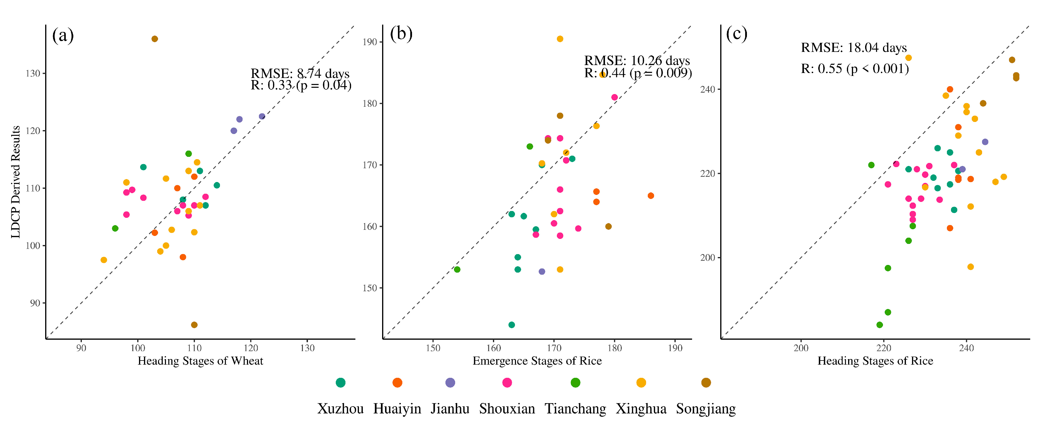
2.6. Validation of the LDCP

To validate our proposed LDCP, we compared the in situ phenological records at seven sites with the corresponding satellite-derived values. As described in Xin et al. [34] and Wang et al. [35], the heading stages of the first-season and the second-season crops corresponded to the peak of the first cropping cycle (i.e., POS1) and the peak of the second cropping cycle (i.e., POS2), in the vegetation indices temporal trajectories, respectively. The emergence stages of the second-season crops corresponded to the troughs of the two neighboring peaks (i.e., SOS2) in the vegetation indices profile. Therefore, we used the heading stages of winter wheat and the second season rice to validate our estimated POS1 and POS2, respectively. We also used the emergence stage of the second season rice to access the accuracy of estimated SOS2. Because there are lots of missing data in the in situ phenological record, and our proposed algorithm may not be able to derive phenological metrics for every year due to the low frequency of good quality Landsat observations, we have different numbers of observations for each individual stages. There are 38, 34, 52 observations for POS1, SOS2, and POS2, respectively.

2.7. Interannual Trends of Phenological Metrics

To understand the interannual variations of double-season cropland phenology, we used a simple linear regression to calculate the trends (i.e., slope) of POS1, SOS2, and POS2 at each pixel from 1993 to 2009, in the four districts of Shanghai. The significance of the linear trends was evaluated using the two-tailed student’s t-test. Time series that were less than 5 years were excluded for the linear regression.

3. Results and Discussions

3.1. Performance of the LDCP

The degree of fitnesses between the observed normalized multi-year EVI and LDCP modeled results were centered at 0.83 ± 0.04, 0.85 ± 0.02, 0.82 ± 0.03, and 0.83 ± 0.03 for Jinshan, Fengxian, Qingpu, and Songjiang district, respectively (Figure S3), indicating that LDCP can effectively capture the temporal trajectories of double-season cropland phenology. The mean and standard deviations of PGQ that correspond to each of the three phenological metrics (i.e., POS1, SOS2, and POS2) were summarized in

Table 1. Mean and standard deviations of the proportion of good quality (PGQ) for POS1, SOS2, and POS2 in the four counties, respectively.

	Jinshan	Fengxian	Qingpu	Songjiang
PGQ of POS1	0.52 ± 0.07	0.59 ± 0.10	0.50 ± 0.09	0.51 ± 0.09
PGQ of SOS2	0.50 ± 0.05	0.48 ± 0.06	0.47 ± 0.06	0.48 ± 0.06
PGQ of POS2	0.50 ± 0.05	0.47 ± 0.06	0.49 ± 0.06	0.49 ± 0.06

. The PGQ for each of the three phenological dates were approximately 50% because the cloud contaminations and SLC-off in the ETM+ sensor reduced the numbers of good quality data in our study areas. Figure S4 exhibits the spatial pattern of PGQ for each of the three phenological dates in the four districts of Shanghai. We can see that PGQ differ greatly across the three phenological dates and have large spatial variations across and within each of the four districts. This indicates that the timing and duration of cloud contaminated days varied a lot in our study regions. We can clearly see a “scan line” effect in the PGQ maps of Jinshan, Qingpu, and Songjiang, which were caused by the SLC-off in Landsat 7 ETM+ sensors (Figure S4). It should be noted that lower PGQ may reduce the quality of the reconstructed time series [36]. However, lower PGQ does not necessarily indicate that the detected phenological metrics (POS1, SOS2, and POS2) are incorrect; it just provides an indicator for the number of good quality data input for the LDCP model.

The key to deriving annual cropland phenology is to successfully identify the $DO{Y}_i$ in Equation (2) within each of the corresponding time intervals: from POS1 to SOS2; from SOS2 to POS2; and from POS2 to end of year (DOY 366). It is possible that we might not be able to detect all three phenological dates for each year due to lack of good quality data, especially back to the time when Landsat ETM+ was not launched, or in regions with persistent cloud cover. The mean and standard deviations of the number of years were summarized in

Table 2. Mean and standard deviations of the number of years that LDCP were able to derive POS1, SOS2, and POS2 in the four counties, respectively.

	Jinshan	Fengxian	Qingpu	Songjiang
No. years of POS1	7.52 ± 2.24	5.57 ± 2.59	5.68 ± 2.58	5.70 ± 2.56
No. years of SOS2	12.42 ± 1.48	11.59 ± 1.95	11.73 ± 1.93	11.60 ± 2.04
No. years of POS2	14.76 ± 0.96	13.97 ± 1.46	14.20 ± 1.49	13.85 ± 1.46

. Figure S5 shows the maps of the number of years that we successfully extracted the annual phenological metrics (i.e., POS1, SOS2, and POS2) of the 17 years in the four districts of Shanghai. Interestingly, there were a greater number of years that LDCP was able to detect phenological metrics of the second cropping cycle (i.e., SOS2 and POS2) than those of the first cropping cycle, despite the fact that the PGQ is similar for the three time intervals (Table 1). This indicates that there was a smaller number of good quality data within the time interval from POS1 to SOS2. One possible reason was that the length of the first cropping cycle (winter wheat or first-season rice) in the study region was generally shorter compared to that of the second cropping cycle (second-season rice).

We compared the derived phenological metrics of the double-season cropland from the LDCP with the phenological stages from the in situ observations (e.g., emergence and heading stages) at seven agro-meteorological stations. We found good agreement between the LDCP-derived metrics and in situ observations for POS1 and SOS2 with RMSE of 8.74 days and 10.26 days, respectively (Figure 3). Although RMSE is larger (18.04 days) for POS2 than the other two metrics, the correlation between POS2 and the heading stages of rice is relatively higher than that of SOS2 and POS1, indicating that there were systematic differences in comparing satellite-derived metrics with ground observations. Discrepancies between the in situ records and derived phenological metrics can exist in reality. The observed phenological metrics provide approximate metrics derived from the time series of remotely sensed images. The ground-based crop observation could only represent site- and species-specific information, while metrics from LDCP are pixel-level (30 m by 30 m) metrics, which could encompass variations induced by agricultural management (multiple rice/wheat types, fertilizer usage, irrigation) and mixed land cover types (e.g., grass, rural roads, rural houses) as a result of landscape heterogeneity. It should be noted that the number of records were different (N = 38, N = 34, N = 52 for POS1, SOS2, and POS2, respectively) for the three metrics, due to missing records in the ground observations.

In addition, LDCP might not derive phenological metrics for every year at the ground stations if no Landsat image is available within any of the three respective periods (see Equation (2)).

There were some potential limitations of the LDCP. We derived annual metrics by shifting the long-term mean, given the deviations of each individual year. It is possible that the growing cycles of the double-cropping system show a complex pattern (e.g., varying rates of crop growth or senescence across different years). However, it is challenging to fit the LDCP to Landsat images acquired in the same year due to lack of data, especially before 2009, when Landsat 8 Operational Land Imager (OLI) was not yet launched. We thus stacked all available images, building upon the success of other examples in the natural forests [17], in order to extend the long-term mean phenology to include the interannual variations at double cropping parcels.

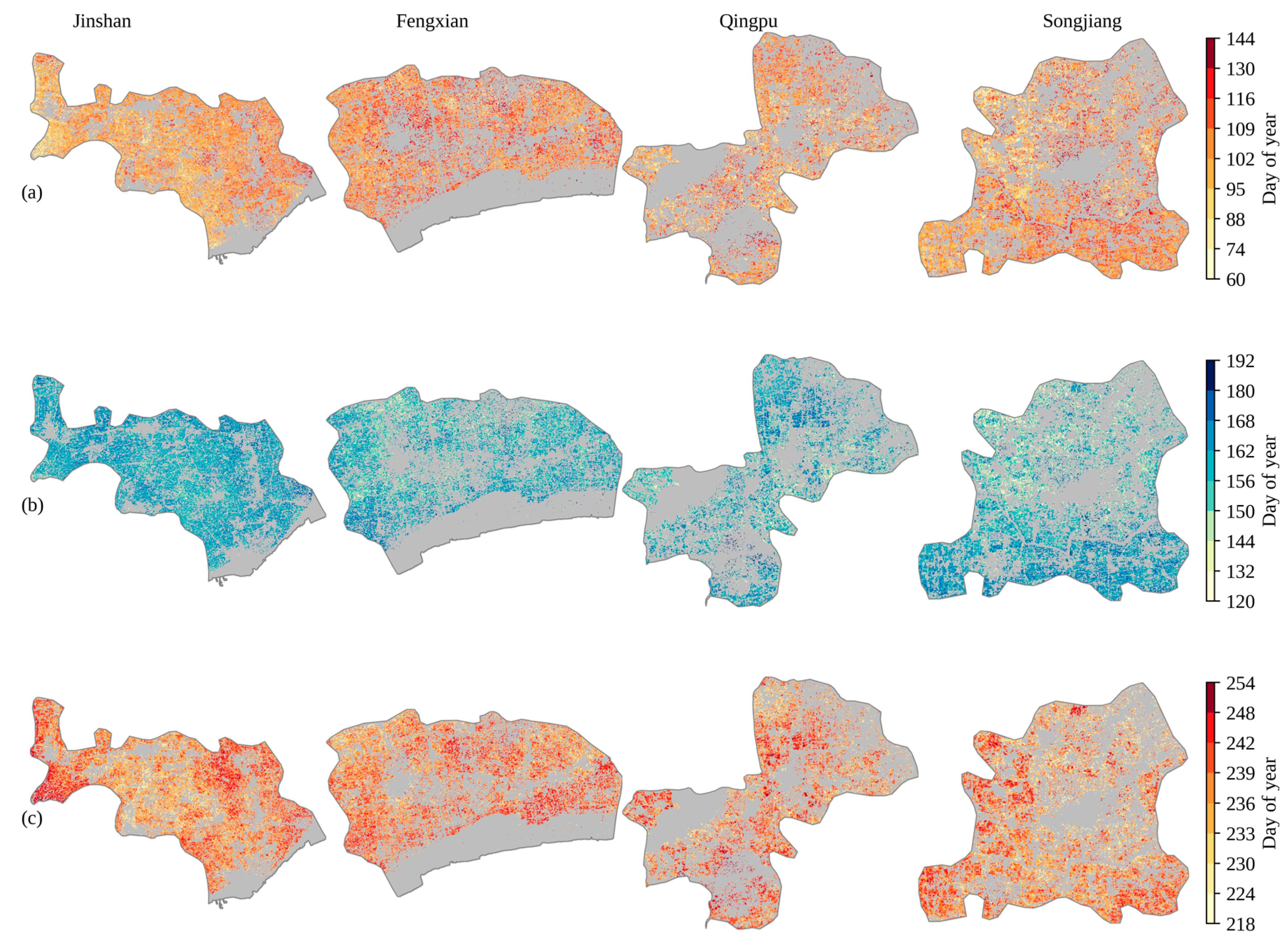
3.2. Maps of Long-Term Mean Double-Season Cropland Phenology

Figure 4 showed the details of three long-term mean phenological metrics in four districts of Shanghai. We can clearly see the spatial heterogeneities at the cropland parcel scales over the landscape, which cannot be captured using coarse spatial resolution sensors such as AVHRR or MODIS. Landsat-derived phenological metrics thus have the potential to provide critical information to retrieve crop growth conditions at parcel scale and improve crop yield estimation. The local variations between two neighboring cropland parcels can be as many as 7–30 days (Figure 4). Several reasons might cause these variations. First, cropland parcel use right (the state owns the cropland) belongs to individual households in China. There are significant variations in agricultural practices for different households, such as the dates of planting, the varieties of rice, the timing and amount of irrigation and fertilization usages, thus introducing variations in cropland phenology. Second, because each Landsat pixel is the average of signals from all features within an area of 900 m², it is thus inevitable that a Landsat pixel may contain cropland parcels from multiple households with different agricultural practices, and possibly some mixtures of other types of LCLU. For example, farmers in China might plant vegetables in their parcels. The seasonal trajectory of vegetables could be significantly different from that of rice and wheat, thus increasing the spatial heterogeneities in the Landsat-scale cropland phenology. Third, noise in the data, possibly due to remnant cloud contamination, might also affect the local variation.

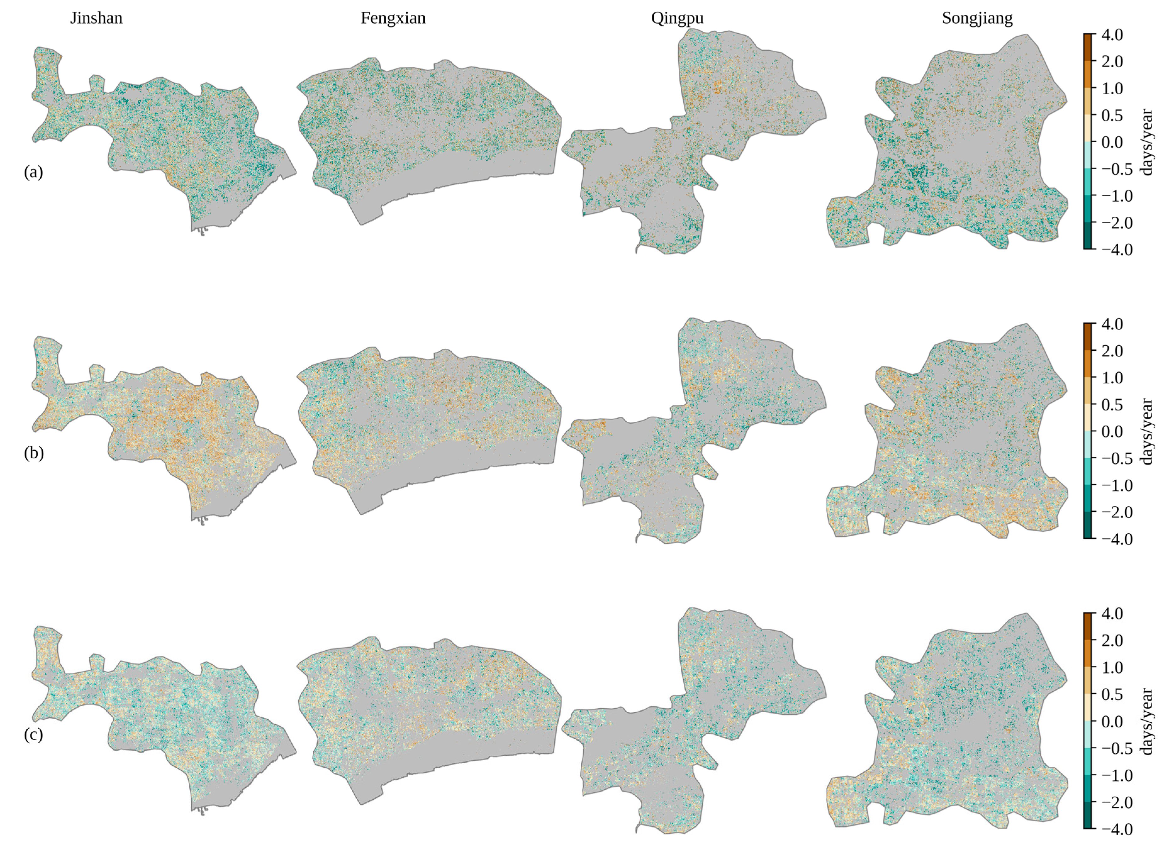
3.3. Interannual Variation of Double-Season Cropland Phenology

Interannual variations of cropland phenology can improve the understanding of the impacts of climate change on crop growth and phenological development. The interannual trends of the phenological metrics from 1993 to 2009 over the four districts are shown in Figure 5. We excluded pixels with less than five years of data in the time series and only plotted the pixels that exhibited a significant trend (p-value < 0.05). Similar to Figure 4, we can observe a spatially heterogeneous temporal trend for each of the three phenological metrics in four districts of Shanghai at Landsat spatial resolution. Two neighboring parcels can exhibit the opposite trend, and the long-term trends of phenological metrics showed a great variation across the four districts. The proportion of significant positive and negative trends for each district were summarized in Figure 6. For POS1, the percentage of significant negative trends was 59.9%, 56.9%, 57.7% in the district of Jinshan, Fengxian, and Songjiang, respectively, indicating that the timing of POS1 was increasingly significantly earlier in most of the regions. Meanwhile, for the Qingpu district, approximately half of the regions had an advanced POS1, while the other half exhibited a delayed POS1. As for SOS2, 68.9%, 55.6%, and 57.2% of the pixels were significantly delayed in the district of Jinshan, Fengxian, and Songjiang, respectively. An earlier POS1 and a later SOS2, mostly in Jinshan, Fengxian, and Songjiang, could indicate a longer growing season for the first crop. Trends of SOS2 in Qingpu district were non-uniform, with approximately half of the regions observed to have an earlier SOS2. As for POS2, Fengxian had a mixed temporal pattern, with 51% of the regions exhibiting earlier POS2. The other three districts, Jinshan, Qingpu, and Songjiang, had advanced POS2 in 59.2%, 60%, and 58.6% of the cropland areas, respectively. Two major factors may explain the temporal trends. First, changes in climatic factors (temperature and precipitation) were reported to influence cropland phenology in China based on ground observations [37,38,39]. Warming temperature in the winter was found to provide favorable growth conditions for cropland (potential driving forces of earlier POS1 and POS2). At the same time, precipitation plays a less important role, because irrigation can greatly increase the soil moisture in the cropland [40]. However, it is challenging to isolate the effects of climate change on Landsat-derived cropland phenology due to the lack of 30-m spatial resolution climate data. The discrepancies in POS1/SOS2 trends between Qingpu and the other three districts could be attributed to the water coverage differences. There were generally more rivers and lakes in Qingpu (Figure 1) than the other three districts, potentially changing the local fluxes of heat and moisture through mesoscale circulation [41] and thus influencing crop growth. For example, studies found that lakes and rivers could reduce the land surface temperature from 2.4–3.3 °C in rural areas, and the maximum cooling distance could reach 440 m and 532 m in spring and summer, respectively [42], which may delay POS1. The second potential factor might be agricultural practice. Studies have documented that crop rotation, irrigation, fertilization, and the introduction of new cultivars can significantly alter the interannual variation of cropland phenology [43,44,45]. The urbanization process in suburban regions of Shanghai might introduce more non-agricultural activities and reduce farm labor availability (i.e., cropland abandonment) [46], thus impacting the agricultural practice and affecting the cropland phenology. For example, SOS2 was mainly determined by the agricultural practice because SOS2 represents the harvesting date of first season crops and the planting date of the second season crops. The harvesting and planting generally required large input of labor in China. The reduced availabilities of farming labors due to urbanization might delay SOS2 in our study sites.

4. Conclusions

In this study, we developed a Landsat double-cropping phenology (LDCP) algorithm to map the phenological stages of double-season cropland at 30-m spatial resolution. We demonstrated the effectiveness of the approach by extracting three key phenological metrics, the peak of first season (POS1), the peak of second season (POS2), and the start of second season (SOS2), in the suburban areas of Shanghai from 1993–2009. We found relatively good agreements between LDCP-derived metrics and the in situ crop development records. We found an advanced peak of season for both cropping cycles (POS1 and POS2) in approximately 50–60% of our study area, while the start of the second season (SOS2) was delayed in approximately 50–70% of the area. These changes reflect the combined effects of agricultural management and climate change on crop phenology.

The phenological metrics derived from LDCP could provide critical information for the timing of irrigation and fertilization usage, thus promoting cropland management and increasing food production. The LDCP has the potential to include other moderate spatial resolution instruments, such as Landsat OLI and Sentinel-2A/B Multispectral Instrument (MSI) [47], or images from high spatial resolution instruments, such as Cubesat [48], to monitor phenological changes at parcel to landscape scales. LDCP can also be used to fully examine the individual and interactive effects of climate change and agricultural management on cropland phenology, given fine grain size climate data that matches with the spatial resolution of Landsat imagery.

References

1. DeFries, R.S.; Foley, J.A.; Asner, G.P. Land-use choices: Balancing human needs and ecosystem function. Front. Ecol. Environ. 2004, 2, 249–257. [Google Scholar] [CrossRef]
2. Tilman, D.; Cassman, K.G.; Matson, P.A.; Naylor, R.; Polasky, S. Agricultural sustainability and intensive production practices. Nature 2002, 418, 671. [Google Scholar] [CrossRef] [PubMed]
3. Sakamoto, T.; Wardlow, B.D.; Gitelson, A.A.; Verma, S.B.; Suyker, A.E.; Arkebauer, T.J. A Two-Step Filtering approach for detecting maize and soybean phenology with time-series MODIS data. Remote Sens. Environ. 2010, 114, 2146–2159. [Google Scholar] [CrossRef]
4. Bolton, D.K.; Friedl, M.A. Forecasting crop yield using remotely sensed vegetation indices and crop phenology metrics. Agric. For. Meteorol. 2013, 173, 74–84. [Google Scholar] [CrossRef]
5. Sakamoto, T.; Gitelson, A.A.; Arkebauer, T.J. MODIS-based corn grain yield estimation model incorporating crop phenology information. Remote Sens. Environ. 2013, 131, 215–231. [Google Scholar] [CrossRef]
6. de Beurs, K.M.; Henebry, G.M. Land surface phenology, climatic variation, and institutional change: Analyzing agricultural land cover change in Kazakhstan. Remote Sens. Environ. 2004, 89, 497–509. [Google Scholar] [CrossRef]
7. Brown, M.E.; de Beurs, K.M.; Marshall, M. Global phenological response to climate change in crop areas using satellite remote sensing of vegetation, humidity and temperature over 26years. Remote Sens. Environ. 2012, 126, 174–183. [Google Scholar] [CrossRef]
8. Sakamoto, T.; Yokozawa, M.; Toritani, H.; Shibayama, M.; Ishitsuka, N.; Ohno, H. A crop phenology detection method using time-series MODIS data. Remote Sens. Environ. 2005, 96, 366–374. [Google Scholar] [CrossRef]
9. Zhang, X.Y.; Friedl, M.A.; Schaaf, C.B.; Strahler, A.H.; Hodges, J.C.F.; Gao, F.; Reed, B.C.; Huete, A. Monitoring vegetation phenology using MODIS. Remote Sens. Environ. 2003, 84, 471–475. [Google Scholar] [CrossRef]
10. Zhang, X.Y.; Friedl, M.A.; Schaaf, C.B. Global vegetation phenology from Moderate Resolution Imaging Spectroradiometer (MODIS): Evaluation of global patterns and comparison with in situ measurements. J. Geophys. Res. Biogeosci. 2006, 111. [Google Scholar] [CrossRef]
11. Gao, F.; Masek, J.; Schwaller, M.; Hall, F. On the blending of the Landsat and MODIS surface reflectance: Predicting daily Landsat surface reflectance. IEEE Trans. Geosci. Remote Sens. 2006, 44, 2207–2218. [Google Scholar] [CrossRef]
12. Gao, F.; Anderson, M.C.; Zhang, X.; Yang, Z.; Alfieri, J.G.; Kustas, W.P.; Mueller, R.; Johnson, D.M.; Prueger, J.H. Toward mapping crop progress at field scales through fusion of Landsat and MODIS imagery. Remote Sens. Environ. 2017, 188, 9–25. [Google Scholar] [CrossRef] [Green Version]
13. Zhu, X.; Chen, J.; Gao, F.; Chen, X.; Masek, J.G. An enhanced spatial and temporal adaptive reflectance fusion model for complex heterogeneous regions. Remote Sens. Environ. 2010, 114, 2610–2623. [Google Scholar] [CrossRef]
14. Pan, Z.; Huang, J.; Zhou, Q.; Wang, L.; Cheng, Y.; Zhang, H.; Blackburn, G.A.; Yan, J.; Liu, J. Mapping crop phenology using NDVI time-series derived from HJ-1 A/B data. Int. J. Appl. Earth Obs. 2015, 34, 188–197. [Google Scholar] [CrossRef] [Green Version]
15. Roy, D.P.; Yan, L. Robust Landsat-based crop time series modelling. Remote Sens. Environ. 2018. [Google Scholar] [CrossRef]
16. Fisher, J.I.; Mustard, J.F.; Vadeboncoeur, M.A. Green leaf phenology at Landsat resolution: Scaling from the field to the satellite. Remote Sens. Environ. 2006, 100, 265–279. [Google Scholar] [CrossRef]
17. Melaas, E.K.; Friedl, M.A.; Zhu, Z. Detecting interannual variation in deciduous broadleaf forest phenology using Landsat TM/ETM plus data. Remote Sens. Environ. 2013, 132, 176–185. [Google Scholar] [CrossRef]
18. Melaas, E.K.; Sulla-Menashe, D.; Gray, J.M.; Black, T.A.; Morin, T.H.; Richardson, A.D.; Friedl, M.A. Multisite analysis of land surface phenology in North American temperate and boreal deciduous forests from Landsat. Remote Sens. Environ. 2016, 186, 452–464. [Google Scholar] [CrossRef]
19. Melaas, E.K.; Sulla-Menashe, D.; Friedl, M.A. Multidecadal Changes and Interannual Variation in Springtime Phenology of North American Temperate and Boreal Deciduous Forests. Geophys. Res. Lett. 2018, 45, 2679–2687. [Google Scholar] [CrossRef]
20. Nijland, W.; Bolton, D.K.; Coops, N.C.; Stenhouse, G. Imaging phenology; scaling from camera plots to landscapes. Remote Sens. Environ. 2016, 177, 13–20. [Google Scholar] [CrossRef]
21. Qiu, T.; Song, C.; Li, J. Impacts of Urbanization on Vegetation Phenology over the Past Three Decades in Shanghai, China. Remote Sens. 2017, 9, 970. [Google Scholar] [CrossRef] [Green Version]
22. Li, X.; Zhou, Y.; Asrar, G.R.; Meng, L. Characterizing spatiotemporal dynamics in phenology of urban ecosystems based on Landsat data. Sci. Total Environ. 2017, 605, 721–734. [Google Scholar] [CrossRef] [PubMed]
23. Li, L.; Friedl, M.; Xin, Q.; Gray, J.; Pan, Y.; Frolking, S. Mapping Crop Cycles in China Using MODIS-EVI Time Series. Remote Sens. 2014, 6, 2473–2493. [Google Scholar] [CrossRef] [Green Version]
24. Zhao, Z.; Sha, Z.; Liu, Y.; Wu, S.; Zhang, H.; Li, C.; Zhao, Q.; Cao, L. Modeling the impacts of alternative fertilization methods on nitrogen loading in rice production in Shanghai. Sci. Total Environ. 2016, 566, 1595–1603. [Google Scholar] [CrossRef] [PubMed]
25. Zhu, Z.; Woodcock, C.E. Object-based cloud and cloud shadow detection in Landsat imagery. Remote Sens. Environ. 2012, 118, 83–94. [Google Scholar] [CrossRef]
26. Huete, A.; Didan, K.; Miura, T.; Rodriguez, E.P.; Gao, X.; Ferreira, L.G. Overview of the radiometric and biophysical performance of the MODIS vegetation indices. Remote Sens. Environ. 2002, 83, 195–213. [Google Scholar] [CrossRef]
27. Verma, M.; Friedl, M.A.; Finzi, A.; Phillips, N. Multi-criteria evaluation of the suitability of growth functions for modeling remotely sensed phenology. Ecol. Model. 2016, 323, 123–132. [Google Scholar] [CrossRef]
28. Anderson, J.; Ardill, R.W.B.; Moriarty, K.J.M.; Beckwith, R.C. A cubic spline interpolation of unequally spaced data points. Comput. Phys. Commun. 1979, 16, 199–206. [Google Scholar] [CrossRef]
29. Chen, J.; Jonsson, P.; Tamura, M.; Gu, Z.H.; Matsushita, B.; Eklundh, L. A simple method for reconstructing a high-quality NDVI time-series data set based on the Savitzky-Golay filter. Remote Sens. Environ. 2004, 91, 332–344. [Google Scholar] [CrossRef]
30. Gray, J.; Friedl, M.; Frolking, S.; Ramankutty, N.; Nelson, A.; Gumma, M.K. Mapping Asian Cropping Intensity With MODIS. IEEE J. Sel. Top. Appl. Earth Obs. Remote Sens. 2014, 7, 3373–3379. [Google Scholar] [CrossRef]
31. Ganguly, S.; Friedl, M.A.; Tan, B.; Zhang, X.; Verma, M. Land surface phenology from MODIS: Characterization of the Collection 5 global land cover dynamics product. Remote Sens. Environ. 2010, 114, 1805–1816. [Google Scholar] [CrossRef] [Green Version]
32. Zhang, X.Y. Reconstruction of a complete global time series of daily vegetation index trajectory from long-term AVHRR data. Remote Sens. Environ. 2015, 156, 457–472. [Google Scholar] [CrossRef]
33. An, S.; Zhang, X.; Chen, X.; Yan, D.; Henebry, G.M. An Exploration of Terrain Effects on Land Surface Phenology across the Qinghai–Tibet Plateau Using Landsat ETM+ and OLI Data. Remote Sens. 2018, 10, 1069. [Google Scholar] [CrossRef] [Green Version]
34. Xin, J.; Yu, Z.; van Leeuwen, L.; Driessen, P.M. Mapping crop key phenological stages in the North China Plain using NOAA time series images. Int. J. Appl. Earth Obs. 2002, 4, 109–117. [Google Scholar] [CrossRef]
35. Wang, J.; Huang, J.-F.; Wang, X.-Z.; Jin, M.-T.; Zhou, Z.; Guo, Q.-Y.; Zhao, Z.-W.; Huang, W.-J.; Zhang, Y.; Song, X.-D. Estimation of rice phenology date using integrated HJ-1 CCD and Landsat-8 OLI vegetation indices time-series images. J. Zhejiang Univ. Sci. B 2015, 16, 832–844. [Google Scholar] [CrossRef] [PubMed]
36. Zhang, X.; Friedl, M.; Schaaf, C. Sensitivity of vegetation phenology detection to the temporal resolution of satellite data. Int. J. Remote Sens. 2009, 30, 2061–2074. [Google Scholar] [CrossRef]
37. Tao, F.; Zhang, Z.; Xiao, D.; Zhang, S.; Rötter, R.P.; Shi, W.; Liu, Y.; Wang, M.; Liu, F.; Zhang, H. Responses of wheat growth and yield to climate change in different climate zones of China, 1981–2009. Agric. For. Meteorol. 2014, 189, 91–104. [Google Scholar] [CrossRef]
38. Tao, F.; Yokozawa, M.; Xu, Y.; Hayashi, Y.; Zhang, Z. Climate changes and trends in phenology and yields of field crops in China, 1981–2000. Agric. For. Meteorol. 2006, 138, 82–92. [Google Scholar] [CrossRef]
39. Tao, F.; Yokozawa, M.; Liu, J.; Zhang, Z. Climate–crop yield relationships at provincial scales in China and the impacts of recent climate trends. Clim. Res. 2008, 38, 83–94. [Google Scholar] [CrossRef]
40. Wang, S.; Mo, X.; Liu, Z.; Baig, M.H.A.; Chi, W. Understanding long-term (1982–2013) patterns and trends in winter wheat spring green-up date over the North China Plain. Int. J. Appl. Earth Obs. 2017, 57, 235–244. [Google Scholar] [CrossRef]
41. Long, Z.; Perrie, W.; Gyakum, J.; Caya, D.; Laprise, R. Northern Lake Impacts on Local Seasonal Climate. J. Hydrometeorol. 2007, 8, 881–896. [Google Scholar] [CrossRef] [Green Version]
42. Wu, C.; Li, J.; Wang, C.; Song, C.; Chen, Y.; Finka, M.; La Rosa, D. Understanding the relationship between urban blue infrastructure and land surface temperature. Sci. Total Environ. 2019, 694, 133742. [Google Scholar] [CrossRef] [PubMed]
43. He, L.; Asseng, S.; Zhao, G.; Wu, D.; Yang, X.; Zhuang, W.; Jin, N.; Yu, Q. Impacts of recent climate warming, cultivar changes, and crop management on winter wheat phenology across the Loess Plateau of China. Agric. For. Meteorol. 2015, 200, 135–143. [Google Scholar] [CrossRef]
44. Xiao, D.; Tao, F. Contributions of cultivars, management and climate change to winter wheat yield in the North China Plain in the past three decades. Eur. J. Agron. 2014, 52, 112–122. [Google Scholar] [CrossRef]
45. Wang, X.H.; Ciais, P.; Li, L.; Ruget, F.; Vuichard, N.; Viovy, N.; Zhou, F.; Chang, J.F.; Wu, X.C.; Zhao, H.F.; et al. Management outweighs climate change on affecting length of rice growing period for early rice and single rice in China during 1991–2012. Agric. For. Meteorol. 2017, 233, 1–11. [Google Scholar] [CrossRef] [Green Version]
46. Zhang, Q.; Song, C.; Chen, X. Effects of China’s payment for ecosystem services programs on cropland abandonment: A case study in Tiantangzhai Township, Anhui, China. Land Use Policy 2018, 73, 239–248. [Google Scholar] [CrossRef]
47. Vuolo, F.; Neuwirth, M.; Immitzer, M.; Atzberger, C.; Ng, W.-T. How much does multi-temporal Sentinel-2 data improve crop type classification? Int. J. Appl. Earth Obs. 2018, 72, 122–130. [Google Scholar] [CrossRef]
48. Houborg, R.; McCabe, M.F. High-Resolution NDVI from Planet’s Constellation of Earth Observing Nano-Satellites: A New Data Source for Precision Agriculture. Remote Sens. 2016, 8, 768. [Google Scholar] [CrossRef] [Green Version]
Figure 1. Our study sites are located in four districts of Shanghai, including Jinshan, Fengxian, Qingpu, and Songjiang. The background is an original raw image of Landsat TM 5 obtained on day of year (DOY) 224 in year 1995, with a band combination 5-4-3. Green colors in the map indicate forest land cover and croplands. Purple colors in the map represent urban and build-up regions.
Remotesensing 12 03275 g001
Figure 2. Schematic demonstration of extracting annual phenological metrics based on multi-year Landsat images. (a) Solid line indicates the multi-year mean fitted line using cubic spline smoothing method. POS1 represents the peak of season of the first cropping cycle, SOS2 indicates the start of season of the second cropping cycles, and POS2 is the peak of season of the second cropping cycle. Colored points stand for normalized enhanced vegetation index (NEVI) in different years. POS1 and POS2 are defined as the first and second peak of the two cropping cycles, respectively. SOS2 is defined as the trough between the two neighboring peaks. Dashed box in panel (a) shows the boundary of the zoom-in plot of panel (b); (b) Solid line is a zoom-in version of the dashed box in panel (a). Dashed line is the fitted phenological curve in year 1996 by shifting multi-year fitted line to the left by 11 days. Eleven days were calculated as the deviation between the acquisition DOY in year 1996 and the DOY of fitted NEVI time series which corresponds to the same NEVI value in year 1996. We did not calculate the mean value of deviation, because there is only one qualified DOY in the year 1996. The POS1 in year 1996 is then calculated by deducting 11 days from the long-term mean POS1.
Remotesensing 12 03275 g002
Figure 3. Validation of LDCP-derived phenological metrics (POS1 for (a), SOS2 for (b), POS2 for (c)) in relation to the in situ phenological stages. Dashed black line is the 1:1 line. Colored points represent results at 7 ground cropland phenology stations. RMSE stands for root mean square error. R represents the correlation between crop stages on the ground and predicted phenological metrics from remote sensing.
Remotesensing 12 03275 g003
Figure 4. Maps of long-term mean phenological metrics in the four counties of Shanghai. Each column in the figure indicates one of the four counties. (a) maps of peak of first cropping cycle (POS1). (b) maps of start of second cropping cycle (SOS2). (c) maps of peak of second cropping cycle (POS2). Gray regions represent missing data and non-crop areas.
Remotesensing 12 03275 g004
Figure 5. Maps of interannual trends of phenological metrics from 1993 to 2009 in the four counties of Shanghai. Each column in the figure indicates one of the four counties. (a) linear trends of peak of first cropping cycle (POS1). (b) linear trends of start of second cropping cycle (SOS2). (c) linear trends of peak of second cropping cycle (POS2). Gray regions represent missing data, non-crop areas, and non-significant regions (p-value > 0.05).
Remotesensing 12 03275 g005
Figure 6. Proportion of significant (p-value < 0.05) positive (slope > 0) and negative (slope < 0) trends of the phenological metrics from 1993 to 2009 in four counties of Shanghai.
Remotesensing 12 03275 g006