GPM-Based Multitemporal Weighted Precipitation Analysis Using GPM_IMERGDF Product and ASTER DEM in EDBF Algorithm

Abstract

To obtain the high-resolution multitemporal precipitation using spatial downscaling technique on a precipitation dataset may provide a better representation of the spatial variability of precipitation to be used for different purposes. In this research, a new downscaling methodology such as the global precipitation mission (GPM)-based multitemporal weighted precipitation analysis (GMWPA) at 0.05° resolution is developed and applied in the humid region of Mainland China by employing the GPM dataset at 0.1° and the Advanced Spaceborne Thermal Emission and Reflection Radiometer (ASTER) 30 m DEM-based geospatial predictors, i.e., elevation, longitude, and latitude in empirical distribution-based framework (EDBF) algorithm. The proposed methodology is a two-stepped process in which a scale-dependent regression analysis between each individual precipitation variable and the EDBF-based weighted precipitation with geospatial predictor(s), and to downscale the predicted multitemporal weighted precipitation at a refined scale is developed for the downscaling of GMWPA. While comparing results, it shows that the weighted precipitation outperformed all precipitation variables in terms of the coefficient of determination (R²) value, whereas they outperformed the annual precipitation variables and underperformed as compared to the seasonal and the monthly variables in terms of the calculated root mean square error (RMSE) value. Based on the achieved results, the weighted precipitation at the low-resolution (e.g., at 0.75° resolution) along-with the original resolution (e.g., at 0.1° resolution) is employed in the downscaling process to predict the average multitemporal precipitation, the annual total precipitation for the year 2001 and 2004, and the average annual precipitation (2001–2015) at 0.05° resolution, respectively. The downscaling approach resulting through proposed methodology captured the spatial patterns with greater accuracy at higher spatial resolution. This work showed that it is feasible to increase the spatial resolution of a precipitation variable(s) with greater accuracy on an annual basis or as an average from the multitemporal precipitation dataset using a geospatial predictor as the proxy of precipitation through the weighted precipitation in EDBF environment.

1. Introduction

Precipitation is the major component of the global water cycle. It is a key parameter of the ecological, hydrological, meteorological and agriculture systems [1,2]. It plays an important role in the energy exchange and material circulation of the Earth surface system [3]. It is of significant importance to understand the characteristics of precipitation, because it shows great variability both in space and time as compared to other climatic variables. Therefore, its spatial and temporal variability greatly influence vegetation distribution, soil moisture and surface runoff [4,5]. In addition, a high-quality precipitation dataset is very important in the development of different ecological and hydrological models at corresponding scales. On top of that, due to certain limiting factors, it is difficult to develop such high-quality dataset(s) from point measurements based on the traditional precipitation, which are as follows: first, the data derived from point measurements heavily depends on field observations [5,6]. Second, field observation stations are not uniformly distributed in space and limited mostly to low and medium altitude areas, with the exception of a few precipitation stations at high altitudes. Moreover, their operational capability is relative for a shorter period. Even if longer precipitation records exist from ground-based stations, they are not sufficient to provide coverage for the global/regional applications, due to deficiencies in reliability of the spatial distribution of precipitation [7], especially over ocean, desert and mountainous areas. Third, a true spatial coverage of precipitation based on the traditional rain gauge observations cannot be obtained [8], because many river basins around the world are still poorly gauged [9], or ungauged [10]. Fourth, it is difficult to effectively reflect the spatial variability of precipitation based on the observation from a finite number of rainfall stations, especially in areas where rainfall stations are sparsely distributed [11,12,13]. Fifth, rain gauge observations can only reflect the point rainfall within a radius around the location of instruments, and the effectiveness of such data is often under question, and adequate validation is further needed [14,15].

Recently, the development in remote sensing and geographic information technology has given a new dimension to present precipitation observations [16,17,18], almost at the global scale over a long period, which also reflects the spatial patterns and temporal variability of precipitation [19]. In this regard, various research institutions and government organizations have developed a series of gridded global precipitation datasets, including Earth observations, in situ datasets and models at both regional and global scales, i.e., the Global Precipitation Climatology Project (GPCP) [2,20,21,22], the Global Satellite Mapping of Precipitation (GSMaP) project [23], the Multi-Source Weighted-Ensemble Precipitation (MSWEP) [24], the Climate Hazards Group InfraRed Precipitation with Station data (CHIRPS) [25], the Precipitation Estimation from Remotely-Sensed Information using Artificial Neural Networks-Climate Record (PERSIANN-CDR) [26], the Tropical Rainfall Measuring Mission (TRMM) [27,28,29], the TRMM Multi-satellite Precipitation Analysis (TMPA) [30], and the Global Precipitation Mission (GPM) [31,32,33].

Spatial downscaling is a recently developed approach to obtain the high spatial resolution of a variable based on conjugation between the variable at a coarse scale and geospatial predictor(s) at the low resolution [34,35]. In this regard, using spatial downscaling techniques on a precipitation dataset may provide a better representation of the spatial variability of precipitation to be used for different purposes. Several authors have used downscaling methodologies to increase the spatial resolution of satellite-based precipitation, often in combination with Earth observations data available on hydro-meteorological variables related to precipitation, including normalized difference vegetation index (NDVI) [30,35,36,37,38,39,40,41,42], digital elevation model [30,38,43,44], land surface temperature [30], soil moisture [37], in situ rain gauged precipitation [37,38], slope [38], aspect [38], and wind [31]. Moreover, few authors have used different satellite-based precipitation datasets for TRMM products [30,42]. Additionally, some studies used regression analysis with model parameters spatially constant (multiple linear, polynomial, exponential, regression kriging, etc.), assuming a spatial stationarity of the relationship between precipitation and the predicting variables [34,35,38,41,44,45,46,47,48]. On top of that, some studies limited their analysis only to satellite-based precipitation datasets and did not take full advantage of all available data sources, combining remotely sensed and in situ observations [42,49,50].

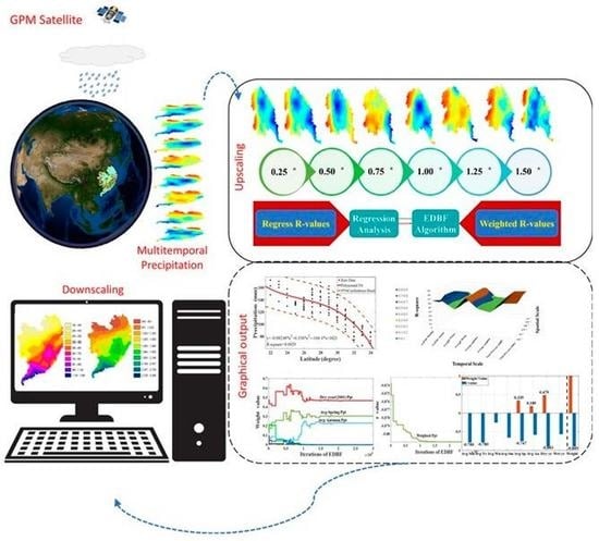
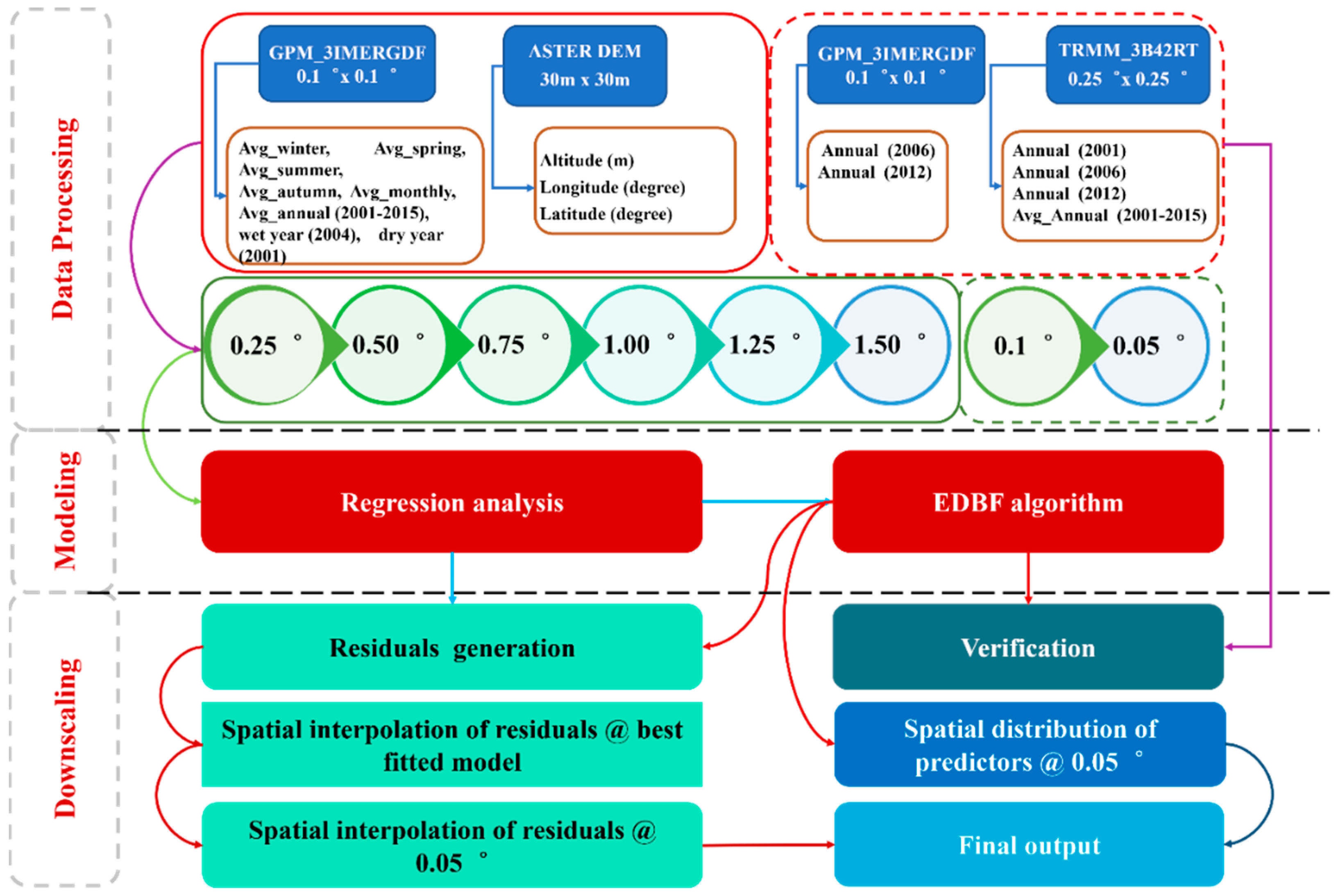
In this research work, a new downscaling methodology (Figure 1), based on the earlier work of [3,38,39], such as the GMWPA is developed using DEM (Figure 2a) to delineate into three geospatial predictors, i.e., elevation, longitude, and latitude [44], in EDBF algorithm. Two different satellite-based precipitation datasets, such as the GPM-based multitemporal precipitation data (Figure 2b–i) for the prediction of high-resolution downscaled weighted precipitation from 0.1° to 0.05° resolution, and the GPM (Figure 2j,k) and the TRMM (Figure 2l–o) datasets for the verification of proposed methodology is used over the humid (the Southern) region of Mainland China. During the execution, certain objectives are set to achieve the required results, which are as follows [51]: to evaluate the multitemporal precipitation (2001–2015) dataset through regression analysis, i.e., polynomial regression at different upscaled resolutions, e.g., 0.25°, 0.5°, 0.75°, 1.0°, 1.25°, 1.50°; (2) based on the regression output, EDBF algorithm is run to evaluate the multitemporal precipitation at each upscaled resolution by assigning weight to each temporal component; (3) to verify the output of EDBF algorithm through the TRMM and the GPM datasets; and (4) to generate the high-resolution downscaled weighted precipitation at 0.05° resolution based on the best performing upscaled resolution. This research can have practical implications, particularly for climate change, drought assessment, and water resources planning, which require long-term precipitation estimates at finer resolution.

2. Materials and Methods

2.1. Study Area

This research is conducted over the Southern part of China, which in Chinese is simply referred to as “the South”. The study area comprises of eight provinces (Anhui, Hunan, Hubei, Jiangxi, Jiangsu, Zhejiang, Fujian, and Guangdong) and one municipality (Shanghai) (Figure 2a). It is approximately the mega-region within China separated by the Qingling-Huaihe Line, which is a reference line used by geographers to distinguish between the Northern and the Southern China, corresponding roughly to 33rd parallel [52]. From Qingling-Huaihe, “Qingling” refers to the Qingling Mountain, and “Huaihe” refers to the Huai River, running from the Qingling Mountain in the West to the Huai River in the East. It divides Eastern China into the North and the South regions, which differ from each other in climate, demography and terrain. All major rivers of China flow across this region, e.g., the Yangtze River, the Huai River, the Han River, the Qu River, the Qiangtang River, the Ou River, the Gan River, the Min River, the Xiang River, the Zi River, the Yuan River and the Lishui River. In addition, some major lakes such as the Dongting Lake, the Tai Lake and the Chaozhou Lake are also located in this region. Moreover, regions laying in the South of the line tend to be tropical and subtropical. Some major mountainous series such as the Huangshan, the Dabie, the She, the Mufu, the Jiuling, the Luoxiao, the Huaiyu, the Wuyi, the Jiulian, the Dayu, the Nong are also located in this region. The Southern part is hotter and wetter than the Northern part. Normally, the weather conditions are with short, cool, damp winters, and very hot, humid summers. The average temperature in winter and summer remains between 3 °C to 9 °C and 27 °C to 30 °C, respectively. The average annual precipitation is between 1200 to 1900 mm, much of it falling in the form of heavy rains occurring in late spring and summer. In addition, half of the most developed tier 1 cities of China are located in the South.

2.2. Datasets

2.2.1. Global Precipitation Mission

During the execution of present study, the Integrated Multi-Satellite Retrievals for GPM (IMERG), an algorithm that provides the multi-satellite precipitation for GPM users, is used to retrieve the required GPM data [33]. Specifically, the daily rainfall (mm day⁻¹) estimate from the GPM Level 3 IMERG *Final* Daily 10 × 10 km Version 06 (GPM_3IMERGDF_V06) is used as primary data, moreover, which is derived from half-hourly GPM_3IMERGHH available at https://giovanni.gsfc.nasa.gov/giovanni/#dataKeyword=IMERGDF (Accessed on 20 June 2020). Besides, the derived result represents the final estimate of the daily accumulated precipitation combined with microwave-infrared. The dataset is produced at the National Aeronautics and Space Administration (NASA) [53], Goddard Earth Sciences [10], Data and Information Services Center (DISC) by simply summing the valid precipitation retrievals for the day in GPM_3IMERGHH and giving the result in (mm). The reason for selecting GPM _IMERG is attributed to following reasons: (i) satellite rainfall estimates with finest gridded data @ 0.1° × 0.1° spatial resolution, high temporal data supply, ranging from half-hourly to daily and monthly, the GPM system provides almost near real-time data with spatial coverage (−180.0, −90.0, 180.0, 90.0) and temporal coverage (2000–06–01 to 2020–03–01). Further details about the GPM _IMERGDF can be found at https://disc.gsfc.nasa.gov/datasets/GPM_3IMERGDF_06/summary?keywords=GPM. (Accessed on 20 June 2020). The daily GPM_3IMERGDF product from 2001 to 2015 is retrieved for the study area into following multitemporal aggregates:

Average Seasonal Precipitation

The daily GPM_3IMERGDF product from 2001 to 2015 is aggregated into the average seasonal precipitation @ 0.1° spatial resolution as shown in Figure 2b–e. The equation deriving the average seasonal precipitation is as follows in Equation (1):

$$P_{GPM\_S}=\frac{{\sum }_{j=1}^m{\sum }_{i=1}^n{P}_{GP{M}_{ij}}}{N}$$

(1)

where $P_{GPM\_S}$ is the average seasonal precipitation which individually corresponds to DJF (December, January and February), MAM (March, April and May), JJA (June, July and August), and SON (September, October and November), respectively. $P_{GP{M}_{ij}}$ is the daily GPM_3IMERGDF precipitation for i-th day, i.e., DJF (n = 90), MAM (n = 92), JJA (n = 92), SON (n = 91) and j-th year (m = 15), and N is the total number of observations. Hence, hereafter, the average winter precipitation for DJF, the average spring precipitation for MAM, the average summer precipitation for JJA, and the average autumn precipitation for SON will be used.

Average Monthly, and Average Annual Precipitation

The daily GPM_3IMERGDF product from 2001 to 2015 is aggregated into the average monthly and the average annual precipitation @ 0.1° spatial resolution as shown in Figure 2f,g, respectively. The equation deriving the average monthly, and the average annual precipitation is as follows in Equation (2):

$$P_{GPM\_Avg}=\frac{{\sum }_{j=1}^m{\sum }_{i=1}^n{P}_{GP{M}_{ij}}}{N}$$

(2)

where $P_{GPM\_Avg}$ is the average monthly and the average annual precipitation for the study area, $P_{GP{M}_{ij}}$ is the daily GPM_3IMERGDF precipitation for i-th day (n = 365) and j-th year (m = 15), and N is the total number of observations (e.g., for the average monthly precipitation N = 180, and for the average annual precipitation N = 15).

Annual Total Precipitation

The daily GPM_3IMERGDF product (365 days) is aggregated into the annual total precipitation for the wet year (2004) and the dry year (2001), and also for the year 2006 and 2012 (i.e., for the verification) @ 0.1° spatial resolution as shown in Figure 2h–k, respectively. The equation deriving the annual total precipitation for the mentioned temporal periods is as follows in Equation (3):

$$P_{GP{M}_i}={\displaystyle \sum }_{j=1}^n{P}_{GP{M}_{daily-j}}$$

(3)

where $P_{GP{M}_i}$ is i-th annual precipitation (i.e., 2001, 2004, 2006 and 2012,) for the study area, $P_{GP{M}_{daily-j}}$ is the daily GPM_3IMERGDF precipitation for j-th day (n = 365).

2.2.2. ASTER Global Digital Elevation Model (GDEM)

The ASTER GDEM is released by the Ministry of Economy, Trade and Industry [53] of Japan, and the NASA [38,54]. The ASTER GDEM covers the land surface between 83°N and 83°S of the Earth, which includes the entire area of Mainland China. The latest GDEM version 3 was released on August 5, 2019, which added additional stereo-pairs with improved coverage and reducing the occurrence of artifacts. The refined production algorithm provides an improved spatial resolution, increased the horizontal and vertical accuracy [53]. It provides the spatial resolution of one arc-second (approximately 30 m), and is used in this study as an influencing predictor on precipitation (Figure 2a). In addition to the elevation data, two other terrain attributes, i.e., longitude and latitude, are also derived from the ASTER GDEM. The ASTER GDEM data is available at https://search.earthdata.nasa.gov/search/granules (Accessed on 20 June 2020).

2.2.3. Tropical Rainfall Measuring Mission

The Tropical Rainfall Monitoring Mission (TRMM) is a joint project between the NASA and the Japan Aerospace Exploration Agency (JAXA). The TRMM was launched on 27th November, 1997 [20,29,55]. It provides measurement for the intensity and areal coverage (60°S to 60°N) of tropical and subtropical precipitation, which covers about two third of the world’s rainfall [38]. There is a range of orbital and gridded TRMM products available, i.e., 3B42RT and 3B43RT datasets [39]. Specifically, the daily rainfall (mm day⁻¹) estimate from the TRMM (TMPA-RT) Near Real-Time Precipitation L3 1day 0.25° × 0.25° Version 7 (TRMM_3B42RT_Daily) is used as the primary dataset during the verification process in the present study, moreover, which is derived from the original three-hour averaged precipitation values available at https://giovanni.gsfc.nasa.gov/giovanni/#service=TmAvMp&starttime=&endtime=&dataKeyword=TRMM (Accessed on 20 June 2020). Further details can be found at https://disc.gsfc.nasa.gov/datasets/TRMM_3B42RT_Daily_7/summary (Accessed on 20 June 2020). The daily TRMM_3B42RT product (365 days) is aggregated into the annual total precipitation for the year 2001, 2006 and 2012 (Figure 2l–n) and the average annual (2001–2015) precipitation (Figure 2o) @ 0.25° spatial resolution, which is used during the verification process. The equation deriving the annual total and the average annual precipitation is given in Equations (2) and (3), respectively.

2.3. Methodology

In this research, a new downscaling methodology (Figure 1) based on the weighted precipitation is presented, at a regional scale, to downscale the multitemporal GPM data in the humid region of Mainland China. To execute the proposed algorithm, a two-stepped methodology is developed to successfully predict and downscale the investigated precipitation variables at a finer scale: first, to evaluate the relationship between each individual precipitation variable and the EDBF-based weighted precipitation with geospatial predictor(s) through regression models; and second, to downscale the predicted multitemporal weighted precipitation at a refined scale.

2.3.1. Pre-Processing of DEM and GPM Datasets

Pre-processing is carried out by extracting geospatial variables, i.e., elevation, longitude, and latitude at 30 m resolution and the GPM-derived precipitation variables, i.e., the average winter, the average spring, the average summer, the average autumn, the average monthly, the average annual (2001–2015), the wet year (2004), and the dry year (2001) precipitation at 0.1° resolution into six different resolution scales (i.e., 0.25°, 0.5°, 0.75°,1°, 1.25°and 1.50°, respectively) by applying the pixel averaging, e.g., the Nearest Neighbor Method. Onward, each scaled image is to be converted into points (Figure S1) for further analysis.

2.3.2. Modeling and Prediction

Regression Analysis

A polynomial regression model is established at all six upscaled resolutions (i.e., also called the low-resolution scales) using geospatial predictors to predict each individual precipitation variable. The equation deriving the relationship between geospatial predictors and precipitation variables at each low-resolution scale is as follows in Equation (4):

$$P_{D. GP{M}_{LR}}=p_1.x_{DE{M}_{LR}}^3+p_2.x_{DE{M}_{LR}}^2+p_3.x_{DE{M}_{LR}}+p_4$$

(4)

where $P_{D.GP{M}_{LR}}$ is the predicted precipitation for each GPM variable at each low-resolution scale, and $p_1, p_2, p_3 and p_4$ are polynomial coefficients, $x_{DE{M}_{LR}}^i$ is the low-resolution geospatial variable(s).

In addition, a linear regression model is established to evaluate the relationship between the EDBF-based weighted precipitation and geospatial predictor, i.e., the latitude, which is as follows in Equation (5):

$$P_{D.WT{P}_{Res}}=p_1.x_{latitude}+p_2$$

(5)

where $P_{D.WT{P}_{Res}}$ is the predicted weighted precipitation at investigated resolution scale(s), e.g., the low-resolution ($P_{D.WT{P}_{LRes}})$ or the high-resolution ($P_{D.WT{P}_{HRes}})$, $p_1 and p_2$ are linear coefficients, and $x_{latitude}$ is the geospatial predictor.

Calculation of r Values

To execute EDBF algorithm for predicting the weighted precipitation from the multitemporal precipitation variables, the generation of initial weight vector for each contributing precipitation variable is a key process. In this regard, the r value is needed to formulate the initial weight vector for each contributing variable. The equation deriving r values at each low-resolution scale is given by Equation (6):

$$r=\frac{Cov\left(P{r}_i, P{r}_j\right)}{\left({\sigma }_{P{r}_i}\times {\sigma }_{P{r}_j}\right)}$$

(6)

where $Cov\left(P{r}_i, P{r}_j\right)$ is the covariance and ${\sigma }_{P{r}_i},{\sigma }_{P{r}_j}$ is the standard deviation of predictors (i, j) at i-th and j-th pixels, respectively. The equation deriving the covariance, the standard deviation and the mean for each investigated predictor is given by Equations (7)–(9), respectively:

$$Cov\left(P{r}_i, P{r}_j\right)=\frac{{\sum }_{ij=1}^n\left(P{r}_i-{\mu }_i\right)\left(P{r}_j-{\mu }_j\right)}{N}$$

(7)

$$\sigma ={\left(\raisebox{1ex}{${\sum }_{i=1}^n{\left(P{r}_i-\mu \right)}^2$}\!\left/ \!\raisebox{-1ex}{$N$}\right.\right)}^{\raisebox{1ex}{$1$}\!\left/ \!\raisebox{-1ex}{$2$}\right.}$$

(8)

$$\mu =\frac{{\sum }_{i=1}^{n}P{r}_i}{N}$$

(9)

where $P{r}_i, P{r}_j$ are the two investigated predictors; ${\mu }_i,{\mu }_j$ are the mean of investigated predictors, respectively, and N is the total number of observations.

Chi-Square ($\chi$²) Test

This is a non-parametric test, which is used for the purpose to check the significance of relationship between each precipitation variable at each low-resolution scale for the assigned weighted values. In this regard, the assumption is made to determine the association between precipitation variables and the low-resolution scales.

The null and alternative hypothesis will be:

H₀: There is a significant relationship between precipitation variables and upscaled resolutions.

H₁: There is no significant relationship between precipitation variables and upscaled resolutions.

The equation deriving chi-square statistic [56], is given by Equation (10):

$${\chi }^2=\left(\raisebox{1ex}{${\sum }_{i=1}^n{\left(O_i-E_i\right)}^2$}\!\left/ \!\raisebox{-1ex}{$E_i$}\right.\right)$$

(10)

where $O_i$ represents the observed, and $E_i$ represents the expected frequency.

Descriptive Statistics

Various statistical parameters are used to verify the proposed methodology by indicating the perfect score and range for each statistical metric, i.e., R², RMSE and the bias (B), which are expressed in Equations (11) and (12):

$$RMSE={\left(\raisebox{1ex}{${\sum }_i^n{\left(O{b}_i-P{r}_i\right)}^2$}\!\left/ \!\raisebox{-1ex}{$n$}\right.\right)}^{\raisebox{1ex}{$1$}\!\left/ \!\raisebox{-1ex}{$2$}\right.}$$

(11)

$$B=\frac{{\sum }_{i=1}^{n}P{r}_i}{{\sum }_{i=1}^{n}O{b}_i}-1$$

(12)

where $O{b}_i$ is the observed variable, $P{r}_i$ is the predicted variable, and n is the number of observations.

2.3.3. EDBF Algorithm

Based on polynomial regression outputs, the most influencing geospatial predictor that predicts multitemporal precipitation variables at each low-resolution scale is considered for further evaluation through EDBF algorithm. In this research, the developed methodology is based on the earlier work of [57,58]. The execution of EDBF algorithm is shown in Figure S2. Based on calculated r values, the process starts through randomly generating initial weight vector W, which by substituting into Equation (13) obtains WTP:

$$WTP=w_M\times M+w_{An}\times An+w_W\times W+w_{Sp}\times Sp+w_{Su}\times Su+w_{Au}\times Au+w_{Wt}\times Wt+w_{Dr}\times Dr$$

(13)

where $WTP$ is the weighted precipitation, W = {$w_M,w_{An},w_W,w_{Sp},w_{Su},w_{Au},w_{Wt},w_{Dr}\}$ corresponds to the weight values (Equation (14)), and vector $M,An,W,Sp,Su,Au,Wt\mathrm{and}Dr$ corresponds to each of the eight precipitation variables, i.e., the average monthly, the average annual, the average winter, the average spring, the average summer, the average autumn, the wet year (2004) and the dry year (2001) precipitation, respectively. Additionally, vector $Re{s}_{0.25},Re{s}_{0.75},Re{s}_{0.50},Re{s}_{1.0},Re{s}_{1.25}\mathrm{and}Re{s}_{1.50}$ corresponds to each low-resolution scale, e.g., 0.25°, 0.5°, 0.75°, 1.0°, 1.25° and 1.50°, respectively:

$$w_M+w_{An}+w_W+w_{Sp}+w_{Su}+w_{Au}+w_{Wt}+w_{Dr}=1$$

(14)

Subsequently, the correlation coefficient $R_{WTP-Re{s}_{0.25}}$, $R_{WTP-Re{s}_{0.50}}$, $R_{WTP-Re{s}_{0.75}}$, $R_{WTP-Re{s}_{1.0}}$, $R_{WTP-Re{s}_{1.25}}\mathrm{and}{R}_{WTP-Re{s}_{1.50}}$ between the WTP and vector $Re{s}_{0.25},Re{s}_{0.50},Re{s}_{0.75},Re{s}_{1.0},Re{s}_{1.25}\mathrm{and}Re{s}_{1.50}$ is calculated, respectively. In addition, EDBF algorithm is run to iteratively optimize W to obtain an accurate weight vector $W_t$, where t represents the number of iterations. Moreover, a relationship (Equation (5)) between WTP and geospatial predictor at vector $Re{s}_{0.25},Re{s}_{0.50},Re{s}_{1.0},Re{s}_{1.25}\mathrm{and}Re{s}_{1.50}$ is evaluated, respectively. Hereafter, the best predicted resolution vector is used in the downscaling process. Similarly, using Equation (5), the same process is repeated for the high-resolution vector $Re{s}_{0.05}$, i.e., 0.05° scale resolution.

3. Results

3.1. Evaluation of GPM-Based Multitemporal Precipitation

The execution of proposed downscaling methodology was first formulated through evaluating the precipitation response, e.g., each GPM-based multitemporal precipitation variable with respect to geospatial predictors at each low-resolution scale. Additionally, each investigated precipitation variable, e.g., the average monthly, the average annual (2001–2015), the average winter, the average spring, the average summer, the average autumn, the dry year (2001) and the wet year (2004) precipitation was plotted against each geospatial predictor at each upscaled resolution. Demonstration through scatter diagrams and polynomial regression (i.e., Figures S3–S5) described the relationship between precipitation variables and geospatial predictors, i.e., elevation, longitude and latitude at upscaled resolutions, respectively. Moreover, the R² values are shown in

Table 1. Output of model fitting between the multitemporal GPM variables and geospatial predictors.

SR	GP	Multitemporal Precipitation
		M	A	Wn	Sp	Su	Au	Wet-y	Dry-y
0.25°	Elevation	0.0804	0.0805	0.0614	0.1636	0.0171	0.0407	0.0567	0.1052
	Longitude	0.0641	0.0636	0.209	0.1473	0.0618	0.1792	0.0476	0.0768
	Latitude	0.6692	0.6684	0.512	0.7974	0.5793	0.5262	0.7416	0.7672
0.50°	Elevation	0.0906	0.0906	0.0573	0.1763	0.0166	0.0452	0.0686	0.1033
	Longitude	0.0527	0.0527	0.1883	0.1314	0.0563	0.1855	0.0414	0.0716
	Latitude	0.5658	0.6558	0.5023	0.786	0.5913	0.5188	0.7422	0.7648
0.75°	Elevation	0.0516	0.0906	0.0516	0.1346	0.0069	0.0372	0.0343	0.0875
	Longitude	0.05	0.05	0.205	0.1488	0.0377	0.1891	0.0358	0.0762
	Latitude	0.6853	0.6853	0.5271	0.8097	0.6148	0.5432	0.7413	0.7848
1.0°	Elevation	0.0579	0.0579	0.0517	0.1534	0.0128	0.041	0.0357	0.1066
	Longitude	0.0722	0.0722	0.2006	0.1328	0.0825	0.1329	0.0686	0.0767
	Latitude	0.6929	0.6929	0.5184	0.8197	0.6415	0.5206	0.7837	0.7848
1.25°	Elevation	0.152	0.152	0.605	0.2963	0.0176	0.0257	0.1025	0.2255
	Longitude	0.0554	0.0554	0.2227	0.1394	0.0708	0.2524	0.0369	0.0656
	Latitude	0.6824	0.6824	0.532	0.8239	0.5685	0.493	0.7814	0.7802
1.50°	Elevation	0.2056	0.2056	0.207	0.2507	0.0646	0.1363	0.1543	0.1867
	Longitude	0.053	0.053	0.2133	0.1143	0.0694	0.24	0.0405	0.0682
	Latitude	0.6179	0.6179	0.4778	0.7699	0.5392	0.5325	0.6889	0.7491

Note: SR stands for the scaled resolution, GP. for geospatial predictors, M for the average monthly, A for the average annual (2001–2015), Wn for the average winter, Sp for the average spring, Su for the average summer, Au for the average autumn, Wet-y for the wet year (2004), Dry-y for the dry year (2001) precipitation, respectively.

, wherein all precipitation variables showed strong response to latitude followed by longitude and elevation, respectively. Furthermore, for the individual precipitation variables, the average spring followed by the dry year (2001) and the wet year (2004) precipitation showed a higher relationship with geospatial predictors, respectively. Apart from geospatial predictors, the highest R² for upscaled resolutions was observed at 1.0° and 0.75°, respectively.

3.2. EDBF-Based Weighted Precipitation

3.2.1. Low-Resolution Weighted Precipitation

Based on initial regression analysis, the most influencing geospatial predictor, namely latitude, was selected to predict the weighted precipitation from the multitemporal precipitation variables via EDBF algorithm. In this regard, r values were calculated (Figure 3a), and used as the basis function to randomly assign initial weight value to each precipitation variable. The reason for negative r values is the existence of a negative relationship between latitude and precipitation variables. Subsequently, the chi-square ($\chi$²) test was employed to evaluate the relationship between precipitation variables at each low-resolution scale for assigned weight values. The ${\chi }_{calculated}^2$ and ${\chi }_{tabulated}^2$ values with 35 degrees of freedom at the significance level (α = 0.05) were 5.267 and 49.802, respectively. Based on statistical results, the ${\chi }_{calculated}^2$˂${\chi }_{tabulated}^2$, thus, the null hypothesis was accepted and rejected the alternative hypothesis. Moreover, it is stated that weight values assigned to precipitation variables were significantly not different. The details can be found in Table S1.

Furthermore, the correlation between precipitation variables and the low-resolution scales was analyzed and is shown in Figure 3b, wherein it showed that the dry year (2001) followed by the average spring, the wet year (2004) and the average summer precipitation are the most influencing variables. As far the scaled resolutions are concerned, 1.0° followed by 0.75° resolution had higher impacts.

Onward, the precipitation data was evaluated through EDBF algorithm, and the number of iterations was set to 3 × 10⁴. Figure 4 demonstrates the iteration wise statistics at each upscaled resolution, in which Figure 4a,d,g,j,m,p show weight values, Figure 4b,e,h,k,n,q show r values, and Figure 4c,f,i,l,o,r show the comparison between weight and r values which were iteratively generated by the algorithm itself. To investigate weight values, it was observed that lots of discrepancies exist in the convergence of investigated variables (e.g., Figure 4a,d,g,j,m,p), and the convergence showed stabilization onward 2 × 10⁴ iterations. In Figure 4a,d,g, the dry year (2001), the average spring and the average autumn; Figure 4j, the dry year (2001), the average spring and the wet year (2004); Figure 4m,p, the dry year (2001), the average autumn and the average spring, respectively, showed higher weight values from the beginning until the last iteration. As far r values are concerned, uncertainty in initial iterations was observed as shown in Figure 4b,e,h,k,n,q, and the convergence showed stabilization onward 1 × 10⁴ iterations. Likewise, it was also observed that r values drastically decreased before the stabilization of convergence.

In addition, the weighted r value predicted by EDBF algorithm was higher as compared to the calculated r value for each precipitation variable, as shown in Figure 4c,f,i,l,o,r. The highest weighted r was predicted at 1.0° (−0.891) followed by 0.75° and 1.25° (−0.889), 0.25° (−0.880), and 0.50° and 1.50° (−0.867), respectively. Nevertheless, the final weight value predicted at all upscaled resolutions was same, e.g., equal to 1, but weighted response towards precipitation variables was not similar. It can clearly be observed that the highest weighted response was given to the dry year (2001) (Figure 4l,i,c,f,r,o) followed by the average spring (Figure 4l,i,o,c,f,r), the average autumn (Figure 4f,r,o,c,i), and the wet year (2004) (Figure 4l), respectively. Finally, the relationship between latitude and the weighted precipitation predicted by EDBF algorithm was shown through scatter plots in Figure 5a–f. In contrast to earlier plots, i.e., the exitance of polynomial relationship between precipitation variables and geospatial predictors, here, the linear relationship was observed. Moreover, the R² between latitude and the weighted precipitation at each upscaled resolution was increased. The higher R² was observed at 1.0°, 1.25°,0.75° resolutions, respectively. Overall, R² was higher than 0.75.

3.2.2. High-Resolution Weighted Precipitation

To predict the weighted precipitation at 0.05° resolution by EDBF algorithm, the same process was adopted as done for the low resolutions. In contrast to predict the low-resolution weighted precipitation, here, the number of iterations was reduced and set to 1000. Figure 6 shows the iteration wise statistics, wherein Figure 6a,b, respectively, show the iteration wise weight values for each precipitation variable and r values. In both figures, the initial discrepancies were observed before the stabilization of convergence onward 600 iterations. On top of that, during the prediction of weighted precipitation, the higher weighted response (Figure 6a,d) was shown by the dry year (2001), the average spring and the average autumn precipitation, respectively. The true picture of weight given to each precipitation variable based on r value was cleared from Figure 6c, wherein it can clearly be observed that the highest weighted response was given to the dry year (2001) ($w_{Dr}$ = 0.507) followed by the average spring ($w_{Sp}$ = 0.220), the average autumn ($w_{Au}$ = 0.151), the average monthly ($w_M$ = 0.050), the average summer ($w_{Su}$ = 0.046), the average winter ($w_W$ = 0.015), the wet year (2004) ($w_{Wt}$ = 0.005) and the average annual (2001–2015) precipitation ($w_{An}$ = 0.002), respectively. Moreover, the comparison between weight and r values are shown in Figure 6d, wherein it showed that the weighted r value predicted by EDBF algorithm is higher as compared to the calculated r value for each precipitation variable, which reflected that the weighted precipitation showed more consistency as compared to individual precipitation variable. Finally, the relationship between the weighted precipitation predicted by EDBF algorithm and latitude (Figure 6e) was shown through scatter plot, and the achieved R² was observed 0.7696.

3.3. Verification Process

3.3.1. Comparison between the Weighted and the Original Multitemporal Precipitation Variables

To compare the EDBF-based weighted precipitation with the GPM-based multitemporal precipitation variables, a linear regression model was established at all upscaled resolutions, e.g., 0.25°, 0.5°, 0.75°, 1.0°, 1.25° and 1.50°. The efficiency comparison was established using three statistical metrics, i.e., R², RMSE, and the bias (B). The results are shown in

Table 2. Comparison between the weighted precipitation and the multitemporal precipitation variables at 0.75° resolution.

Variables	Statistical Parameters
	R-Square	Mean	S. D.	RMSE	Bias
Weighted Ppt	0.792	897.680	295.860	135.005	−3.0E−06
Avg-Monthly	0.609	125.319	25.335	15.836	−3.6E−05
Avg-Annual	0.609	1503.828	304.016	190.043	2.8E−05
Avg-Winter	0.533	181.795	70.273	48.041	4.5E−05
Avg-Summer	0.426	617.508	123.003	93.165	8.1E−06
Avg-Spring	0.559	466.215	160.574	106.693	−0.00012
Avg-Autumn	0.333	241.951	47.712	38.959	−2.2E−05
Wet-Y (2004)	0.316	1308.082	258.892	214.166	1.9E−05
Dry-Y (2001)	0.781	1452.542	514.112	240.376	0.00010

(e.g., 0.75° resolution) and Table S2 (0.25°, 0.5°, 1.0°, 1.25° and 1.50°), respectively. From the tabulated results, it was observed that for the achieved R² value, the weighted precipitation outperformed all multitemporal variables at all upscaled resolutions. The highest R² value of 0.794 was observed at 1.0° followed by 0.792 at 0.75° resolution, respectively. Also, for the achieved RMSE value, the weighted precipitation outperformed the annual precipitation variables, such as the average annual (2001–2015), the wet year (2004) and the dry year (2001) precipitation, whereas it underperformed compared to the seasonal, e.g., the average winter, the average spring, the average summer and the average autumn precipitation, and the monthly precipitation variables. The lowest RMSE value (i.e., at all upscaled resolutions) was observed for the average monthly precipitation. Moreover, the observed bias for the two precipitation datasets, e.g., the weighted precipitation and the multitemporal precipitation variables, was almost reaching zero. In addition, both precipitation datasets were also compared at the original 0.1° resolution as shown in

Table 3. Comparison between the weighted precipitation and multitemporal precipitation variables original 0.1° resolution.

Variables	Statistical Parameters
	R-Square	Mean	S. D.	RMSE	Bias
Weighted Ppt	0.772	920.915	295.731	141.113	8.89E−05
Avg-Monthly	0.591	124.681	25.084	16.044	2.17E−05
Avg-Annual	0.591	1496.164	301.015	192.537	3.3E−05
Avg-Winter	0.510	181.066	70.465	49.303	−0.00034
Avg-Summer	0.407	612.638	119.603	92.099	−5.1E−06
Avg-Spring	0.561	464.828	159.760	105.901	−5.2E−05
Avg-Autumn	0.299	241.260	49.556	38.979	3.78E−07
Wet-Y (2004)	0.307	1306.001	255.948	212.987	−3.2E−05
Dry-Y (2001)	0.766	1440.258	503.257	243.108	−5.7E−05

. The tabulated results revealed the same outcome as in Table 2, wherein the best correlation (R²) was observed between latitude and the weighted precipitation, and it outperformed all multitemporal precipitation variables. Similarly, for the achieved RMSE value, it outperformed the annual precipitation variables and underperformed compared to the seasonal and the monthly variables. As a whole, the observed output at each statistical parameter for each precipitation variable was slightly reduced from lower to higher (e.g., from Table 2 to Table 3) resolution.

3.3.2. Verification of the Weighted Precipitation with Neutral Variables

The weighted precipitation was further evaluated by comparing with neutral variables which were not used during the prediction of EDBF-based weighted precipitation. In this regard, the precipitation variables from two different datasets, such as the TRMM and the GPM, were used for the verification of weighted precipitation. The GPM dataset used during verification comprised of the annual 2006 (Figure 2j) and 2012 (Figure 2k) precipitation, whereas the TRMM dataset comprised of the annual 2001, 2006, 2012 and the average annual (2001–2015) (Figure 2l–o) precipitation, respectively. The verification of weighted precipitation though the GPM data was evaluated by extracting precipitation at the original 0.1° resolution, whereas through the TRMM data, it was evaluated at the original 0.25° resolution. The verification results are shown in

Table 4. Comparison between the weighted precipitation and neutral precipitation variables.

Variables	Statistical Parameters
	R-Square	Mean	S. D.	RMSE	Bias
Weighted Ppt @ 0.1°	0.772	920.915	295.731	141.113	8.8E−05
GPM (2006)	0.668	1555.048	463.560	267.117	−0.00013
GPM (2012)	0.391	1687.073	517.823	404.087	4.3E−05
Weighted Ppt @ 0.25°	0.776	868.975	281.890	133.377	9.5E−06
TRMM (2001)	0.599	1393.780	480.101	303.951	−1.8E−05
TRMM (2012)	0.318	1668.233	546.886	451.363	−1.1E−05
TRMM (2006)	0.473	1608.031	542.391	393.678	−2.1E−05
Avg-TRMM (01-15)	0.373	1534.130	374.400	296.581	−2.7E−05

. The weighted precipitation outperformed both, as can be observed by comparing the datasets, by achieving a higher R² value of 0.776 at 0.25° resolution and 0.772 at 0.1° resolution as compared to the TRMM and the GPM-based precipitation, respectively. Subsequently, the weighted precipitation also produced lower RMSE, e.g., 133.37 (0.25° resolution) and 141.113 (0.1° resolution) as compared to the TRMM- and the GPM-based precipitation, respectively. Apart from that, the observed bias almost reached zero for all variables, wherein the weighted precipitation showed positive bias, while the TRMM and the GPM precipitation showed negative bias.

3.4. Downscaling of the Weighted Precipitation

Based on the verification of EDBF results, the algorithm was employed in the downscaling process. During the downscaling process, a distinction between the low-resolution (upscaling) and the high-resolution (downscaling) was made by using Equation (5). By subtracting the weighted precipitation $P_{D.WT{P}_{LR}}$ (i.e., also called the low-resolution weighted precipitation) (Figure 7b) from the original $Avg\_M{T}_{GPM}$ precipitation (Figure 7a), the residuals $\left(R_{WT{P}_{LR}}\right)$ of the regression model (i.e., also called as the low-resolution weighted residuals) at 0.75° resolution were obtained as shown in Figure 7c, which represents the amount of precipitation that could not be predicted by the weighted precipitation via EDBF algorithm according to Equation (15). Subsequently, the generated residuals were interpolated to 0.05° resolution (Figure 7d), also called the high-resolution weighted residuals ($R_{WT{P}_{HR}}$), by applying a spline tension interpolator [59]. Finally, the high-resolution weighted precipitation ($P_{D.WT{P}_{HR}}$) at 0.05° resolution (Figure 7e) was obtained using Equation (5). Using Equation (16) to add the high-resolution weighted precipitation to the high-resolution weighted residuals, the final downscaled high-resolution weighted precipitation $P_{Ds.PWT{P}_{HR}}$ (Figure 7f) for the humid region of Mainland China was obtained:

$$R_{WT{P}_{LR}}=Av{g}_{GPM}-P_{D.WT{P}_{LR}}$$

(15)

$$P_{Ds.PWT{P}_{HR}}=P_{D.WT{P}_{HR}}+R_{WT{P}_{HR}}$$

(16)

4. Discussion

In this study, a new downscaling methodology, namely GMWPA at 0.05° resolution, was developed and investigated in the humid region of Mainland China. A two-stepped procedure [38,39,41], based on a scale-dependent regression analysis and downscaling of the predicted multitemporal weighted precipitation at a refined scale, was adopted during the execution of proposed methodology. For this purpose, the multitemporal GPM precipitation dataset (2001 to 2015) at 0.1° and ASTER 30 m DEM-based geospatial predictors, i.e., elevation, longitude, and latitude were taken as input variables to predict the low-resolution—for the residual generation at optimal resolution scale—and the high-resolution weighted precipitation, and were used in the final downscaling process.

Furthermore, the regression analysis was performed in two phases. In the first phase, each geospatial predicator was assessed through developing a relationship (Table 1) with each individual precipitation variable via a fitting line—polynomial fit. Moreover, it was observed that latitude showed the highest correlation with all precipitation variables and achieved the highest R² value. Compared to previous studies [3,34,59] which used either one or two independent variables (NDVI, elevation), the authors in [38] used several independent variables, i.e., latitude, longitude, elevation, slope, aspect, NDVI, Max_NDVI, Range_NDVI, and Min_NDVI, to establish regression models for deriving the annual precipitation over continental China. From the study, it was concluded that, apart from latitude, all variables including NDVI showed relatively weak empirical relationships with the observed precipitation, especially over the humid region of China. Specifically, for NDVI, a possible reason may be that NDVI-related predictors are better indicator of precipitation in arid and semi-arid areas. The NDVI values would not increase with the increased rainfall amount in humid areas, which makes a relatively weak empirical relationship between precipitation and saturated NDVI. Keeping in view, latitude was selected as the proxy of precipitation and employed in assigning initial weight value (e.g., based on r value calculated for each precipitation variable with respect to latitude) to each individual precipitation variable from the multitemporal precipitation dataset, and which was then processed in EDBF algorithm [58] to predict the weighted precipitation.

Likewise, in the second phase, the output precipitation variable from EDBF, e.g., the weighted precipitation was assessed via developing the relationship with latitude through linear fitting. Moreover, the correlation between latitude and the weighted precipitation was increased for each of the low-resolution scale, and the highest R² was achieved at 100 km (e.g., between 0.75°, 1.0°, 1.25° resolutions), which showed that the weighted precipitation was well captured by latitude at 100 km resolution. Although the highest correlation between latitude and the weighted precipitation was achieved at 1.0° (100 km), but due to certain reasons, 0.75° resolution was selected as an optimal low resolution (e.g., for the upscaling) during the downscaling process. First, there was not much difference between the two resolution scales for the achieved R², i.e., 0.75° (R² = 0.7918) and 1.0° (R² = 0.7977) resolution. Secondly, 0.75° resolution had more pixels, i.e., 195, as compared to 111 pixels for 1.0° resolution to cover the whole study area. Considering, to convert points into pixels, the Spline Interpolation method [51,60] was used, which estimates values using a mathematical function that minimizes the overall surface curvature, resulting in a smooth surface that passes exactly through a specified number of nearest input points while passing through the sample points. Thus, using 0.75° resolution, which had a closer specified number of nearest input points, i.e., 12 points, than 1.0° resolution, tends to produce a smoother surface by minimizing the surface curvature.

From the EDBF algorithm perspective, it is a general framework rather than a specific algorithm, which is easy to implement and can easily accommodate any existing multi-parent crossover algorithms (MCAs). Moreover, the existing MCA-based coefficients [61,62,63] follow a uniform distribution, which also violates constraints, thus propagate error. Errors cascade exponentially, with even a slight increase in the hybrid scale, which leads to the increase in time consumption. To address such problem, EDBF is the best solution which takes multiple MCAs as its constituent members. In addition, the number of iterations during the execution of EDBF algorithm at the low-resolution scale, i.e., 0.25°, 0.50°, 0.75°, 1.0°, 1.25° and 1.50° was set to 3 × 10⁴ with the reason that a possible number of iterations be available for the stabilization of convergence before the ending of simulation process. Moreover, the process was repeated for all the low resolutions. Though the convergence stabilized before a 3 × 10⁴ number of iterations, still a slight improvement could be observed, and further improvement in the regression value(s) could be expected. Instead, by terminating simulation during the execution, we let simulation process to be completed until the last iteration. Owing to that, the number of iterations was reduced during the simulation of high-resolution (i.e., 0.05° resolution) weighted precipitation, and the convergence was well stabilized within the set number of iterations.

During the verification process, the weighted precipitation was first compared with its contributing multitemporal precipitation variables at all the low and the original resolution scales. It outperformed all input variables for the achieved R² and outperformed the annual precipitation and underperformed compared to the seasonal and the monthly precipitation variables for the achieved RMSE. Furthermore, the weighted precipitation was compared with different classified precipitations, extracted either as an individual or grouped variables from the original multitemporal precipitation dataset used in the prediction of EDBF-based weighted precipitation at the original 0.1° resolution. The results are shown in

Table 5. Comparison between the weighted precipitation and classified extracted precipitation variables.

Variables	Statistical Parameters
	R-Square	Mean	S. D.	RMSE	Bias
Weighted Ppt	0.772	920.915	295.731	141.113	8.8E−05
Avg-MT Ppt	0.708	1096.535	250.712	135.370	5.8E−06
Avg-An (01-15) + Wet + Dry Ppt	0.696	1414.141	325.185	179.248	−2.1E−05
Avg-An (01-15) + Dry Ppt	0.726	1468.211	394.319	206.353	−9.4E−05
Avg-An (01-15) + Wet Ppt	0.511	1401.083	261.236	182.762	1.2E−05
Wet + Dry Ppt	0.728	1373.130	341.383	178.025	1.2E−05
Avg-An (01-15)	0.591	1496.164	301.015	192.537	3.3E−05
Avg-MT (-01 & -04) Ppt	0.558	1515.092	297.221	197.434	−2.9E−05

Note: Avg-MT Ppt is the average multitemporal precipitation; Avg-An(01-15) + Wet + Dry Ppt is the average precipitation as product of the average annual, the wet year (2004) and the dry year (2001) precipitation; Avg-An + Dry Ppt is the average precipitation as product of the average annual (2001–2015) and the dry year (2001) precipitation; Avg-An(01-15) + Wet Ppt is the average precipitation as product of the average annual (2001–2015) and the wet year (2004) precipitation; Wet + Dry Ppt is the average precipitation as product of the wet year (2004) and the dry year (2001) precipitation; Avg-An (01-15) is the average annual (2001–2015) precipitation; Avg-MT(-01 & -04) Ppt is the average multitemporal precipitation excluding the dry year (2001) and the wet year (2004) precipitations.

, in which the weighted precipitation showed the highest correlation with its predictor (R² = 0.772) as compared to other used variables. In addition, the weighted precipitation had a lower RMSE value (e.g., RMSE = 141.113 mm) than the Avg-An (01–15) + Wet Ppt+ Dry Ppt, Avg-An (01–15) + Dry Ppt, Avg-An (01–15) + Wet Ppt, Wet Ppt + Dry Ppt, Avg-An (01–15) and Avg-MT (−01 & −04) Ppt with the observed RMSE value of 179.248, 206.353, 182.762, 178.025, 192.537 and 197.434 mm, respectively. Also, it had a higher RMSE than the Avg-MT Ppt variable, i.e., 135.370 mm. The reason of low RMSE value for the average multitemporal GPM precipitation was that the average output was equally contributed by each precipitation variable from the multitemporal dataset. Out of the eight used variables from the multitemporal precipitation dataset, the five variables consisted of the seasonal and the monthly precipitation, which had lower received pixel precipitation. Adding to this, the number of days counted during each of the seasonal component (e.g., average 90 days) is lower than the annual component (e.g., 365 days) and there is less probability of variation in the seasonal precipitation than the annual precipitation. Despite lower R² values, less variability from the mean precipitation was observed in the seasonal and the monthly precipitation as compared to the annual precipitation. On the contrary, the EDBF-based weighted precipitation was mainly predicted on the basis of assigned weights via calculated r values. In this regard, higher the r value, the more weight was assigned to that variable and more contribution from that variable in the prediction of weighted precipitation. Additionally, it was compared with neutral variables, wherein it outperformed all comparing variables for the achieved R² and RMSE values.

The downscaling methodology applied in this study was mainly based on the work presented in [39], where the basis function was selected at an optimum resolution and by interpolating the residuals. After successfully applying the proposed methodology, the EDBF algorithm was employed in downscaling of the dry year (2001), the wet year (2004) and the average annual (2001–2015) precipitation at 0.05° resolution by following the same process as for downscaling the $Avg\_M{T}_{GPM}$ precipitaiton. Before downscaling, a graphical relationship between the weighted precipitiaon and the dry year (2001), the wet year (2004) and the average annual (2001–2015) precipitation was developed through a scatter plot as shown in Figure 5g–i, respectively. The weighted precipitation showed the highest correlation with the dry year (2001) followed by the average annual (2001–2015) and the wet year (2004) for the achieved R² = 0.9869, 0.8929 and 0.4154, respectively.

Moreover, during downscaling, the low-resolution weighted residuals (Figure S6d–f) were generated by subtracting the low-resolution weighted precipitation $P_{D.WT{P}_{LR}}$ (Figure 7b) from the original dry year (2001), the wet year (2004) and the average annual (2001–2015) precipitation (Figure S6a–c) at 0.75° resolution, respectively. Afterward, the high-resolution weighted residuals (Figure S6g–i) at 0.05° were obtained by interpolating the low-resolution residuals at 0.75° resolution. 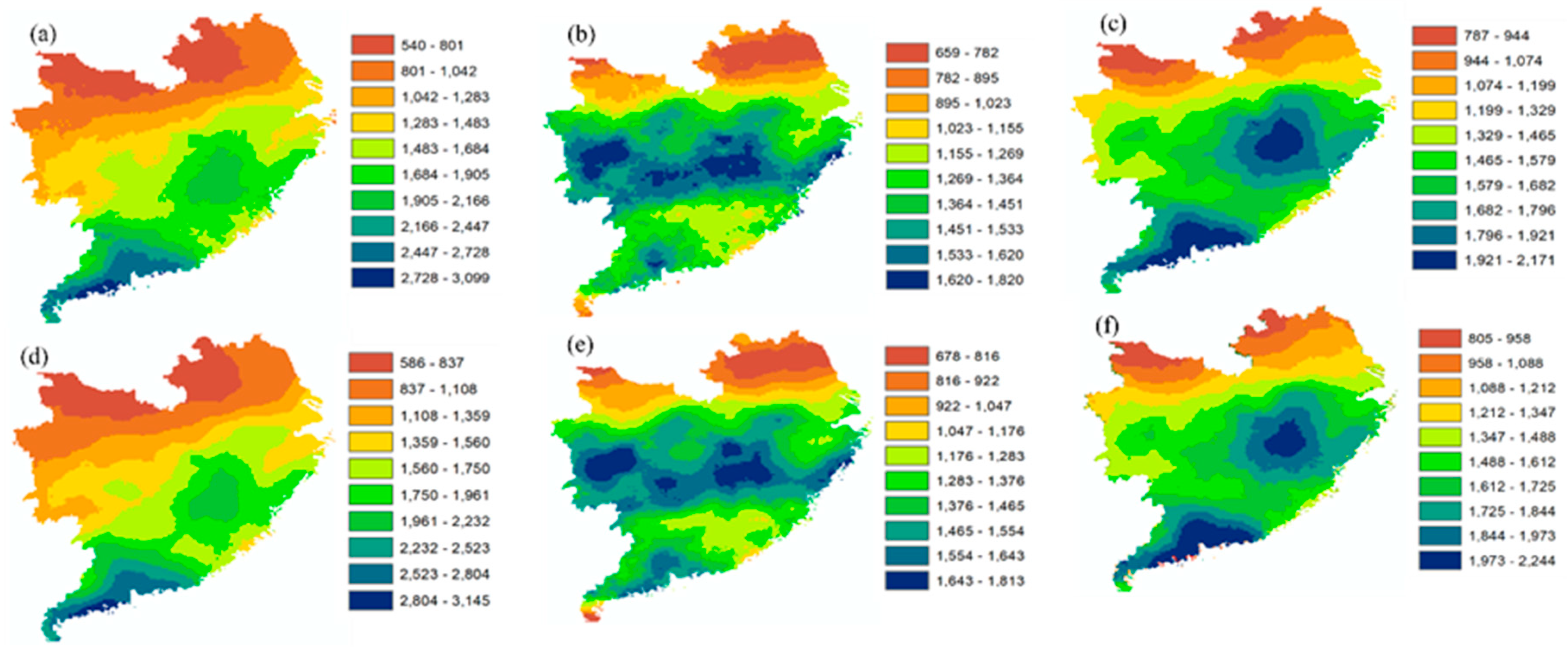Finally, by adding the obtained high-resolution interpolated residuals to the high-resolution weighted precipitation (Figure 7e), the downscaled high-resolution weighted precipitation at 0.05° resolution for the dry year (2001) (Figure 8d), the wet year (2004) (Figure 8e) and the average annual (2001–2015) precipitation (Figure 8f) was obtained. From Figure 8, it shows that the high-resolution weighted precipitation captured the same precipitation pattern as that of the original GPM dry year (2001), the wet year (2004) and the average annual (2001–2015) precipitation at 0.1°. Moreover, by analyzing the class wise pattern (

Table 6. Comparison of spatial pattern between GPM based precipitations with its corresponding weighted precipitation for different precipitation classes.

Variables	Precipitation Classes
GPM 2001	540	801	1042	1283	1483	1684	1905	2166	2447	2728
	801	1042	1283	1483	1684	1905	2166	2447	2728	3099
	261	241	241	200	201	221	261	281	281	371
Weighted 2001	586	837	1108	1359	1560	1750	1961	2232	2523	2804
	837	1108	1359	1560	1750	1961	2232	2523	2804	3145
	251	271	251	201	190	211	271	291	281	341
GPM 2004	659	782	895	1023	1155	1269	1364	1451	1533	1620
	782	895	1023	1155	1269	1364	1451	1533	1620	1820
	123	113	128	132	114	95	87	82	87	200
Weighted 2004	676	816	922	1047	1176	1283	1376	1465	1554	1643
	816	922	1047	1176	1283	1376	1465	1554	1643	1813
	140	106	125	129	107	93	89	89	89	170
Avg-Annual (2001–2015)	787	944	1074	1199	1329	1465	1579	1682	1796	1921
	944	1074	1199	1329	1465	1579	1682	1796	1921	2171
	157	130	125	130	136	114	103	114	125	250
Weighted Avg-Annual (2001–2015)	805	958	1088	1212	1347	1488	1612	1725	1844	1973
	958	1088	1212	1347	1488	1612	1725	1844	1973	2244
	153	130	124	135	141	124	113	119	129	271

Green colored values show the average difference of less than 5 mm, Blue colored values show the average difference of about 10 mm, Pink colored values show the average difference of about 20 mm, Red colored values show the average difference of about 30 mm between the GMP and weighted precipitation at particular pattern class, respectively.

) for the obtained precipitation, the algorithm accurately captured the wet year (2004) (Figure 8e) and the average annual (2001–2015) precipitation, whereas some classes, e.g., class 4 (gold color) and 5 (light green) were not very well captured during downscaling of the dry year (2001) precipitation, such as between 111° to 115°E and 25° to 27°N, and 117° to 118°E and 24° to 25°N.

Subsequently, to analyze difference in the range of precipitation classes (i.e., difference between the upper and the lower boundary of captured precipitation pattern) between the original dry year (2001), the wet year (2004) and the average annual (2001–2015) precipitation at 0.1° resolution, their corresponding weighted precipitation at 0.05° resolution was found to be in close proximity with the average difference of less than 5 mm for most classes. Apart from that, EDBF algorithm slightly underpredicted extreme precipitation for the dry year (2001) and the wet year (2004) with the average difference of 30 mm, and overpredicted the average annual (2001–2015) precipitation with a difference of 20 mm. On the contrary, for low precipitation EDBF underpredicted the dry year (2001) and the average annual (2001–2015), and overpredicted the wet year (2004) precipitation with the average difference of 10, 4 and 23 mm, respectively. Similarly, considering the individual precipitation variable, EDBF accurately predicted the wet year (2003) and the average annual (2001–2015) precipitation with the average difference of less than 5 mm, whereas it slightly overpredicted the dry year (2001) with an average difference of 10 mm between the original and the corresponding weighted precipitation.

5. Conclusions

This study investigated and developed a new downscaling methodology, such as GMWPA at 0.05° resolution based on the multitemporal GPM precipitation dataset (2001 to 2015) at 0.1° and ASTER 30 m DEM-based geospatial predictors, i.e., elevation, longitude, and latitude in EDBF algorithm. The proposed methodology is a two-stepped process: (i) to develop a scale dependent relationship between precipitation variables, i.e., the multitemporal GPM precipitation and the weighted precipitation, and geospatial predictors through regression analysis [45]; (ii) the downscaling of EDBF-based multitemporal weighted precipitation at a refined scale. In addition, EDBF results were validated using neutral variables, e.g., the GPM-based annual 2006 and 2012 precipitation, the TRMM-based annual (2001, 2006 and 2012) and the average annual (2001–2015) precipitation. The following conclusions are drawn from this work:

• Geospatial predictors were the proxy of precipitation and polynomial function best described the relationship between the multitemporal precipitation variables and geospatial predictors, i.e., elevation, longitude, and latitude.
• The correlation between the multitemporal GPM variables and geospatial predictors varies with resolution, and the best correlation was found at a resolution of approximately 100 km (0.75°–1.25°). The highest correlation between precipitation variables and geospatial predictors was observed for the average spring followed by the dry year (2001) and the wet year (2004) precipitation, respectively. The latitude showed to be the best geospatial predictor.
• The weighted r value predicted by EDBF algorithm was higher than the calculated r value for each of the individual precipitation variables. The highest weighted r value was predicted at 1.0° (−0.891) followed by 0.75°and 1.25° (−0.889), respectively. Besides, the highest weighted response was observed for the dry year (2001), followed by the average spring, the average autumn and the wet year (2004), respectively.
• In contrast to the priori polynomial relationship between the multitemporal precipitation variables and geospatial predictors, a consistent linear relationship between the weighted precipitation and latitude was observed with an R² value of 0.7696, 0.7761, 0.7697, 0.7918, 0.7944, 0.7919 and 0.7517 at 0.05°, 0.25°, 0.50°, 0.75°, 1.0°, 1.25° and 1. 50° resolution, respectively.
• In comparison with the multitemporal GPM variables, the weighted precipitation outperformed all variables for the achieved R² value, whereas it outperformed the annual precipitation variables and underperformed compared to the seasonal and the monthly variables for the achieved RMSE value. In addition, it outperformed all comparing variables during the verification process for the achieved R² and RMSE values.
• Based on achieved results, the downscaling process was carried out for the average multitemporal precipitation, the multitemporal annual precipitation (2001 and 2004) and the average annual precipitation (2001–2015).
• The proposed downscaling methodology was refined through earlier methodologies described in [3,39,64] by selecting the basis function at an optimum resolution and by interpolating the residuals.
• The downscaling approach resulted through the proposed methodology captured spatial patterns with greater accuracy at higher spatial resolution.
• This work showed that it is feasible to increase the spatial resolution and accuracy of a precipitation variable on an annual basis or as an average from the multitemporal precipitation dataset using a geospatial predictor, i.e., latitude as the proxy of precipitation through the weighted precipitation. Future work should focus on extending this procedure using the multitemporal precipitation dataset from multi-satellites or a satellite combining rain gauge precipitation, also through analyzing the combined effect of predictors (e.g., geospatial and environmental, etc.) as the proxy of precipitation.

In conclusion, it is possible to accurately downscale the GPM-based multitemporal precipitation using geospatial predictors in the humid region (Southern China) of Mainland China and that the presented methodology is generic in nature and is applicable in all climatic conditions of the world.

References

1. Langella, G.; Basile, A.; Bonfante, A.; Terribile, F. High-resolution space–time rainfall analysis using integrated ANN inference systems. J. Hydrol. 2010, 387, 328–342. [Google Scholar] [CrossRef]
2. Lopez, P.; Immerzeel, W.; Rodríguez Sandoval, E.; Sterk, G.; Schellekens, J. Spatial downscaling of satellite-based precipitation and its impact on discharge simulations in the Magdalena River Basin in Clombia. Front. Earth Sci. 2018, 6, 68. [Google Scholar] [CrossRef] [Green Version]
3. Jia, S.; Zhu, W.; Lu, A.; Yan, T. A statistical spatial downscaling algorithm of TRMM precipitation based on NDVI and DEM in the Qaidam Basin of China. Remote Sens. Environ. 2011, 115, 3069–3079. [Google Scholar] [CrossRef]
4. Li, M.; Shao, Q. An improved statistical approach to merge satellite rainfall estimates and rain gauge data. J. Hydrol. 2010, 385, 51–64. [Google Scholar] [CrossRef]
5. Goodrich, D.; Faurès, J.; Woolhiser, D.; Lane, L.; Sorooshian, S. Measurement and analysis of small-scale convective storm rainfall variability. J. Hydrol. 1995, 173, 283–308. [Google Scholar] [CrossRef]
6. Wheater, H.; Isham, V.; Cox, D.; Chandler, R.; Kakou, A.; Northrop, P.; Oh, L.; Onof, C.; Rodriguez-Iturbe, I. Spatial-temporal rainfall fields: Modelling and statistical aspects. Hydrol. Earth Syst. Sci. 2000, 4, 581–601. [Google Scholar] [CrossRef] [Green Version]
7. Gruber, A.; Levizzani, V. Assessment of global precipitation products: A project of the World Climate Research Programmed Global Energy and Water Cycle Experiment (GEWEX) Radiation Panel; WCRP-128; WMO: Geneva, Switzerland, 2008; p. 50. [Google Scholar]
8. Wilheit, T. Some comments on passive microwave measurement of rain. Bull. Am. Meteorol. Soc. 1986, 67, 1226–1232. [Google Scholar] [CrossRef]
9. Loukas, A.; Vasiliades, L. Streamflow simulation methods for ungauged and poorly gauged watersheds. Nat. Hazard Earth Syst. Sci. 2014, 14, 1641. [Google Scholar] [CrossRef] [Green Version]
10. Sivapalan, M.; Takeuchi, K.; Franks, S.; Gupta, V.; Karambiri, H.; Lakshmi, V.; Liang, X.; McDonnell, J.; Mendiondo, E.; O’connell, P. IAHS decade on Predictions in Ungauged Basins (PUB), 2003–2012: Shaping an exciting future for the hydrological sciences. Hydrol. Sci. J. 2010, 48, 857–880. [Google Scholar] [CrossRef] [Green Version]
11. Beesley, C.; Frost, A.; Zajaczkowski, J. A comparison of the BAWAP and SILO spatially interpolated daily rainfall datasets. In Proceedings of the 18th World IMACS/MODSIM Congress, Cairns, Australia, 13–17 July 2009. [Google Scholar]
12. Hughes, D. Comparison of satellite rainfall data with observations from gauging station networks. J. Hydrol. 2006, 327, 399–410. [Google Scholar]
13. Jeffery, S. Error Analysis for the interpolation of monthly rainfall used in the generation of SILO rainfall datasets; Technical Report; The Queensland Department of Natural Resources: Brisbane City, Australia, 2006. [Google Scholar]
14. Collischonn, B.; Collischonn, W.; Tucci, C.E.M. Daily hydrological modeling in the Amazon basin using TRMM rainfall estimates. J. Hydrol. 2008, 360, 207–216. [Google Scholar] [CrossRef]
15. Bohnenstengel, S.I.; Schlünzen, K.; Beyrich, F. Representativity of in situ precipitation measurements–A case study for the LITFASS area in North-Eastern Germany. J. Hydrol. 2011, 400, 387–395. [Google Scholar] [CrossRef]
16. Dingman, S. Physical Hydrology; Prentice Hall: New Jersey, NJ, USA, 2002. [Google Scholar]
17. Michaelides, S.; Levizzani, V.; Anagnostou, E.; Bauer, P.; Kasparis, T.; Lane, J. Precipitation: Measurement, remote sensing, climatology and modeling. Atmos. Res. 2009, 94, 512–533. [Google Scholar] [CrossRef]
18. Nastos, P.; Kapsomenakis, J.; Philandras, K. Evaluation of the TRMM 3B43 gridded precipitation estimates over Greece. Atmos. Res. 2016, 169, 497–514. [Google Scholar] [CrossRef]
19. Adler, R.; Kidd, C.; Petty, G.; Morissey, M.; Goodman, H. Inter-comparison of global precipitation products: The third Precipitation Inter-comparison Project (PIP-3). Bull. Am. Meteorol. Soc. 2001, 82, 1377–1396. [Google Scholar]
20. Huffman, G.; Adler, R.; Arkin, P.; Chang, A.; Ferraro, R.; Gruber, A.; Janowiak, J.; McNab, A.; Rudolf, B.; Schneider, U. The global precipitation climatology project (GPCP) combined precipitation dataset. Bull. Am. Meteorol. Soc. 1997, 78, 5–20. [Google Scholar] [CrossRef]
21. Huffman, G.; Adler, R.; Morrissey, M.; Bolvin, D.; Curtis, S.; Joyce, R.; McGavock, B.; Susskind, J. Global precipitation at one-degree daily resolution from multisatellite observations. J. Hydrometeorol. 2001, 2, 36–50. [Google Scholar] [CrossRef] [Green Version]
22. Huffman, G.; Adler, R.; Bolvin, D.; Gu, G. Improving the global precipitation record: GPCP version 2.1. Geophys. Res. Lett. 2009, 36. [Google Scholar] [CrossRef] [Green Version]
23. Kubota, T.; Shige, S.; Hashizume, H.; Aonashi, K.; Takahashi, N.; Seto, S.; Hirose, M.; Takayabu, Y.; Ushio, T.; Nakagawa, K. Global precipitation map using satellite-borne microwave radiometers by the GSMaP project: Production and validation. IEEE Trans. Geosci. Remote Sens. Environ. 2007, 45, 2259–2275. [Google Scholar] [CrossRef]
24. Beck, H.; Van Dijk, A.; Levizzani, V.; Schellekens, J.; Gonzalez Miralles, D.; Martens, B.; De Roo, A. MSWEP: 3-hourly 0.25 global gridded precipitation (1979–2015) by merging gauge, satellite, and reanalysis data. Hydrol. Earth Syst. Sci. 2017, 21, 589–615. [Google Scholar] [CrossRef] [Green Version]
25. Funk, C.; Peterson, P.; Landsfeld, M.; Pedreros, D.; Verdin, J.; Shukla, S.; Husak, G.; Rowland, J.; Harrison, L.; Hoell, A. The climate hazards infrared precipitation with stations—A new environmental record for monitoring extremes. Sci. Data 2015, 2, 1–21. [Google Scholar] [CrossRef] [Green Version]
26. Hsu, K.-L.; Gao, X.; Sorooshian, S.; Gupta, H. Precipitation estimation from remotely sensed information using artificial neural networks. J. Appl. Meteorol. 1997, 36, 1176–1190. [Google Scholar] [CrossRef]
27. Kummerow, C.; Barnes, W.; Kozu, T.; Shiue, J.; Simpson, J. The tropical rainfall measuring mission (TRMM) sensor package. J. Atmos. Ocean. Technol. 1998, 15, 809–817. [Google Scholar] [CrossRef]
28. Kummerow, C.; Simpson, J.; Thiele, O.; Barnes, W.; Chang, A.; Stocker, E.; Adler, R.; Hou, A.; Kakar, R.; Wentz, F. The status of the Tropical Rainfall Measuring Mission (TRMM) after two years in orbit. J. Appl. Meteorol. 2000, 39, 1965–1982. [Google Scholar] [CrossRef]
29. Huffman, G.; Bolvin, D.; Nelkin, E.; Wolff, D.; Adler, R.; Gu, G.; Hong, Y.; Bowman, K.; Stocker, E. The TRMM multisatellite precipitation analysis (TMPA): Quasi-global, multiyear, combined-sensor precipitation estimates at fine scales. J. Hydrometeorol. 2007, 8, 38–55. [Google Scholar] [CrossRef]
30. Ma, Z.; Shi, Z.; Zhou, Y.; Xu, J.; Yu, W.; Yang, Y. A spatial data mining algorithm for downscaling TMPA 3B43 V7 data over the Qinghai–Tibet Plateau with the effects of systematic anomalies removed. Remote Sens. Environ. 2017, 200, 378–395. [Google Scholar] [CrossRef]
31. Mahmud, M.; Mohd Yusof, A.; Mohd Reba, M.; Hashim, M. Mapping the daily rainfall over an ungauged tropical micro-watershed: A downscaling algorithm using GPM data. Water 2020, 12, 1661. [Google Scholar]
32. Hou, A.; Kakar, R.; Neeck, S.; Azarbarzin, A.; Kummerow, C.; Kojima, M.; Oki, R.; Nakamura, K.; Iguchi, T. The global precipitation measurement mission. Bull. Am. Meteorol. Soc. 2014, 95, 701–722. [Google Scholar] [CrossRef]
33. Huffman, G.; Stocker, E.; Bolvin, D.; Nelkin, E.; Tan, J. GPM IMERG Final Precipitation L3 1 day 0.1 degree × 0.1 degree V06. In Goddard Earth Sciences Data and Information Services Center (GES DISC); Andrey, G., Savtchenko, M.D., Eds.; NASA: Washington, DC, USA, 2019. [Google Scholar]
34. Duan, Z.; Bastiaanssen, W. First results from Version 7 TRMM 3B43 precipitation product in combination with a new downscaling–calibration procedure. Remote Sens. Environ. 2013, 131, 1–13. [Google Scholar] [CrossRef]
35. Hunink, J.; Immerzeel, W.; Droogers, P. A High-resolution Precipitation 2-step mapping Procedure (HiP2P): Development and application to a tropical mountainous area. Remote Sens. Environ. 2014, 140, 179–188. [Google Scholar] [CrossRef]
36. Zhang, Q.; Shi, P.; Singh, V.; Fan, K.; Huang, J. Spatial downscaling of TRMM-based precipitation data using vegetative response in Xinjiang, China. Int. J. Climatol. 2017, 37, 3895–3909. [Google Scholar] [CrossRef]
37. Ulloa, J.; Ballari, D.; Campozano, L.; Samaniego, E. Two-step downscaling of TRMM 3B43 V7 precipitation in contrasting climatic regions with sparse monitoring: The case of Ecuador in Tropical South America. Remote Sens. 2017, 9, 758. [Google Scholar] [CrossRef] [Green Version]
38. Shi, Y.; Song, L.; Xia, Z.; Lin, Y.; Myneni, R.; Choi, S.; Wang, L.; Ni, X.; Lao, C.; Yang, F. Mapping annual precipitation across Mainland China in the period 2001–2010 from TRMM 3B43 product using spatial downscaling approach. Remote Sens. 2015, 7, 5849–5878. [Google Scholar] [CrossRef] [Green Version]
39. Immerzeel, W.; Rutten, M.; Droogers, P. Spatial downscaling of TRMM precipitation using vegetative response on the Iberian Peninsula. Remote Sens. Environ. 2009, 113, 362–370. [Google Scholar] [CrossRef]
40. Chen, F.; Liu, Y.; Liu, Q.; Li, X. Spatial downscaling of TRMM 3B43 precipitation considering spatial heterogeneity. Int. J. Remote Sens. 2014, 35, 3074–3093. [Google Scholar] [CrossRef]
41. Alexakis, D.; Tsanis, I. Comparison of multiple linear regression and artificial neural network models for downscaling TRMM precipitation products using MODIS data. Environ. Earth Sci. 2016, 75, 1077. [Google Scholar] [CrossRef]
42. Ceccherini, G.; Ameztoy, I.; Hernández, C.; Moreno, C. High-resolution precipitation datasets in South America and West Africa based on satellite-derived rainfall, enhanced vegetation index and digital elevation model. Remote Sens. 2015, 7, 6454–6488. [Google Scholar] [CrossRef] [Green Version]
43. Goovaerts, P. Geostatistical approaches for incorporating elevation into the spatial interpolation of rainfall. J. Hydrol. 2000, 228, 113–129. [Google Scholar] [CrossRef]
44. Zhang, Y.; Li, Y.; Ji, X.; Luo, X.; Li, X. Fine-resolution precipitation mapping in a mountainous watershed: Geostatistical downscaling of TRMM products based on environmental variables. Remote Sens. 2018, 10, 119. [Google Scholar] [CrossRef] [Green Version]
45. Fang, J.; Du, J.; Xu, W.; Shi, P.; Li, M.; Ming, X. Spatial downscaling of TRMM precipitation data based on the orographical effect and meteorological conditions in a mountainous area. Adv. Water Resour. 2013, 61, 42–50. [Google Scholar] [CrossRef]
46. Park, N. Spatial downscaling of TRMM precipitation using geostatistics and fine scale environmental variables. Adv. Meteorol. 2013, 2013, 237126. [Google Scholar] [CrossRef]
47. Chen, C.; Zhao, S.; Duan, Z.; Qin, Z. An improved spatial downscaling procedure for TRMM 3B43 precipitation product using geographically weighted regression. IEEE J. Sel. Top. Appl. Earth Obs. Remote Sens. 2015, 8, 4592–4604. [Google Scholar] [CrossRef]
48. Xu, G.; Xu, X.; Liu, M.; Sun, A.; Wang, K. Spatial downscaling of TRMM precipitation product using a combined multifractal and regression approach: Demonstration for South China. Water 2015, 7, 3083–3102. [Google Scholar] [CrossRef] [Green Version]
49. Ezzine, H.; Bouziane, A.; Ouazar, D.; Hasnaoui, M. Downscaling of open coarse precipitation data through spatial and statistical analysis, integrating NDVI, NDWI, ELEVATION, and distance from sea. Adv. Meteorol. 2017, 2017, 8124962. [Google Scholar] [CrossRef] [Green Version]
50. Xu, S.; Wu, C.; Wang, L.; Gonsamo, A.; Shen, Y.; Niu, Z. A new satellite-based monthly precipitation downscaling algorithm with non-stationary relationship between precipitation and land surface characteristics. Remote Sens. Environ. 2015, 162, 119–140. [Google Scholar] [CrossRef]
51. Mitas, L.; Mitasova, H. General variational approach to the interpolation problem. Comput. Math. Appl. 1988, 16, 983–992. [Google Scholar] [CrossRef] [Green Version]
52. Li, S.; Yang, S.; Liu, X. Spatiotemporal variability of extreme precipitation in north and south of the Qinling-Huaihe region and influencing factors during 1960–2013. Prog. Geogr. 2015, 34, 354–363. [Google Scholar]
53. NASA; METI; AIST; Japan Space System. ASTER Global Digital Elevation Model V003. NASA EOSDIS Land Processes DAAC. 2019. Available online: https://cmr.earthdata.nasa.gov/search/concepts/C1299783579-LPDAAC_ECS.html (accessed on 20 June 2020).
54. Ullah, S.; Farooq, M.; Sarwar, T.; Tareen, M.J.; Wahid, M.A. Flood modeling and simulations using hydrodynamic model and ASTER DEM—A case study of Kalpani River. Arab. J. Geosci. 2016, 9, 439. [Google Scholar] [CrossRef]
55. Huffman, G.; Adler, R.; Bolvin, D.; Nelkin, E. The TRMM Multi-satellite Precipitation Analysis (TMPA), in Chapter 1. In Satellite Rainfall Applications for Surface Hydrology; Springer: Dordrecht, The Netherlands, 2010. [Google Scholar]
56. Miller, R.; Siegmund, D. Maximally selected Chi-square statistics. Biometrics 1982, 38, 1101–1106. [Google Scholar] [CrossRef]
57. Ahn, C.W.; Ramakrishna, R.S. Elitism-based compact genetic algorithms. IEEE Trans. Evol. Comput. 2003, 4, 367–385. [Google Scholar]
58. Zuo, Z.; Yan, L.; Ullah, S.; Sun, S.; Zhang, R.; Zhao, H. Empirical distribution based framework for improving multi-parent crossover algorithms. Soft Comput. 2020, in press. [Google Scholar]
59. Verlinde, J. TRMM Rainfall Data Downscaling in the Pangani Basin in Tanzania; Delft University of Technology: Delft, The Netherlands, 2011. [Google Scholar]
60. Franke, R. Smooth interpolation of scattered data by local thin plate splines. Comput. Math. Appl. 1982, 8, 237–281. [Google Scholar] [CrossRef] [Green Version]
61. Eiben, A.E.; Back, T. Empirical investigation of multiparent recombination operators in evolution strategies. Evol. Comput. 1997, 5, 347–365. [Google Scholar] [CrossRef] [PubMed]
62. Herrera, F.; Lozano, M.; Verdegay, J.L. Tackling real-coded genetic algorithms: Operators and tools for behavioral analysis. Artif. Intell. Rev. 1998, 12, 265–319. [Google Scholar] [CrossRef]
63. Goldberg, D.E. Real-coded genetic algorithms, virtual alphabets, and blocking. Complex Syst. 1991, 5, 139–167. [Google Scholar]
64. Agam, N.; Kustas, W.P.; Anderson, M.C.; Li, F.; Neale, C.M.U. A vegetation index based 572 technique for spatial sharpening of thermal imagery. Remote Sens. Environ. 2007, 107, 545–558. [Google Scholar] [CrossRef]
Figure 1. Proposed methodology to predict the high-resolution downscaled weighted precipitation.
Remotesensing 12 03162 g001
Figure 2. The dataset required for downscaling of the multitemporal precipitation: (a) the DEM of study area; (b) the GPM-based average winter precipitation; (c) the GPM-based average spring precipitation; (d) the GPM-based average summer precipitation; (e) the GPM-based average autumn precipitation; (f) the GPM-based average monthly precipitation; (g) the GPM-based average annual (2001–2015) precipitation; (h) the GPM-based wet year (2004) precipitation; (i) the GPM-based dry year (2001) precipitation, (j) the GPM-based annual (2006) precipitation; (k) the GPM-based annual (2012) precipitation; (l) the TRMM-based annual (2001) precipitation; (m) the TRMM-based annual (2006) precipitation; (n) the TRMM-based annual (2012) precipitation; (o) the TRMM-based average annual (2001–2015) precipitation, respectively.
Remotesensing 12 03162 g002
Figure 3. Selection of initial input parameters for EDBF) algorithm to predict the weighted precipitation (a) calculated r values, and (b) the correlation between precipitation variables and the low-resolution scales for assigned weight values.
Remotesensing 12 03162 g003
Figure 4. Execution of EDBF algorithm at different low-resolution scales, (a,d,g,j,m,p) iteratively estimated weighted values, (b,e,h,k,n,q) iteratively estimated r values, and (c,f,i,l,o,r) the comparison between assigned weights and estimated r values at 0.25°, 0.50°, 0.75°, 1.0°, 1.25°, 1.50° resolutions, respectively.
Remotesensing 12 03162 g004
Figure 5. Scaled wise relationship between the weighted precipitation and (a) latitude at 0.25° resolution; (b) latitude at 0.50° resolution; (c) latitude at 0.75° resolution; (d) latitude at 1.0° resolution; (e) latitude at 1.25° resolution; (f) latitude at 1.50° resolution; (g) the dry year (2001) precipitation at 0.75° resolution; (h) the wet year (2006) precipitation at 0.75°; and (i) the average annual (2001–2015) precipitation at 0.75°, respectively.
Remotesensing 12 03162 g005
Figure 6. Execution of EBDF algorithm for predicting the high-resolution weighted precipitation at 0.05° resolution: (a) iteratively estimated weight values; (b) iteratively estimated r values; (c) the estimated final weight values; (d) the comparison between the estimated weights and r values; and (e) the relationship between the weighted precipitation and latitude, respectively.
Remotesensing 12 03162 g006
Figure 7. Stepwise downscaling process to predict the high-resolution multitemporal weighted precipitation: (a) the GPM-based average multitemporal precipitation at 0.75° resolution; (b) the EDBF-based weighted precipitation at 0.75° resolution; (c) the low-resolution weighted residuals at 0.75° resolution generated from the difference between (a) and (b); (d) the high-resolution weighted residuals at 0.05° resolution generated by interpolating (c) via Spline Interpolation; (e) the EDBF-based high-resolution weighted precipitation at 0.05° resolution; and (f) the final high-resolution downscaled multitemporal weighted precipitation, at 0.05° resolution, as a product of adding (d) into (e), respectively.
Remotesensing 12 03162 g007
Figure 8. Comparison between the downscaled weighted precipitation at 0.05° resolution for (d)(e)(f) and the original GPM precipitation at a nominal resolution of 0.1° for (a) the dry year (2001), (b) the wet year (2004), and (c) the average annual (2001–2015), respectively.
Remotesensing 12 03162 g008